1 Introduction

Hubert Aaronson’s wide ranging contributions to materials science over the last four decades has focussed repeatedly on three major topics and their applications to phase transformations:[1, 2, 3, 4, 5, 6, 7]

1) solution thermodynamics and multicomponent phase equilibria;[8, 9, 10, 11]

2) equilibrium shapes of surfaces with anisotropic surface energy;[12, 13, 14, 15, 16, 17, 18, 19, 20, 21] and,

3) the morphology of growing precipitates.[22, 23, 24, 25]

In this paper, we hope to honor Hub and his contributions by illustrating how each of these topics derives from a common mathematical basis and that the graphical constructions derived for each separately can shed new insight into the others.

Tangent constructions are powerful graphical methods, widely used for heuristic, computational and theoretical purposes in our field.[26, 27, 2] We will look at differences in how tangent constructions are used in each of three topics, and explore how these varied methods may be used in the others.

For multicomponent phase equilibria (at constant temperature and pressure) the tangent construction is performed on a plot of the molar Gibbs free energy, $G(\mbox{$\vec{c}$})$, which has to be convex from below at equilibrium. (Here $\mbox{$\vec{c}$}=(c_{1},c_{2},...)$ is a short-hand [vector] notation for the molar composition of a multicomponent phase or system.) For first order phase changes, $G(\mbox{$\vec{c}$})$ may be multivalued with a different $G(\mbox{$\vec{c}$})$ for each phase, usually with a different symmetry. Concavities in this plot represent metastable and unstable phases and compositions for which the free energy is too high. Such concavities lead to ranges in composition (sometimes called miscibility gaps) where single phases are not in equilibrium. These concavities are removed with the common tangent construction, that identifies for a particular average composition whether a single phase is in equilibrium, and if not what mix of phases will have the lowest free energy. This graphical process, termed convexification, leads to a convex hull of $G(\mbox{$\vec{c}$})$. Each point on that convex hull represents the lowest free energy of the system of a given average composition, including permitting the equilibrium to be multiphase. Common tangents are often used to construct phase diagrams from a nonconvex $G(\mbox{$\vec{c}$})$.

A quite similar set of graphical procedures is applied to the orientation dependent surface free energy per unit area $\gamma(\mbox{$\vec{n}$})$, except that the construction is performed on a radial plot of the reciprocal of $\gamma(\mbox{$\vec{n}$})$ [28] . Here $\mbox{$\vec{n}$}=(n_{1},n_{2},n_{3})$ is the normal to the surface. Note that the components of $\vec{n}$ are the analogs of the concentrations of the chemical species.[29] Concavities are removed by convexification, and the points on the convex hull of $1/\mbox{$\gamma(\mbox{$\vec{n}$})$}$ represent (the reciprocal of) the lowest free energy a surface with a certain average orientation can achieve. Interface orientations for which $1/\mbox{$\gamma(\mbox{$\vec{n}$})$}$ lies inside the convex hull have too high an energy and are unstable. The tangent construction identifies which surfaces become corrugated at equilibrium, and specifies which orientations of lower energy coexist to replace a high energy surface, even though there is greater surface area. If there is more than one possible phase state of the surface (facetted, surface melted, wetted, etc.) $\gamma(\mbox{$\vec{n}$})$ may be multivalued, just as $G(\mbox{$\vec{c}$})$. The convexification of $1/\mbox{$\gamma(\mbox{$\vec{n}$})$}$ has many analogies to that for $G(\mbox{$\vec{c}$})$: It identifies the occurrence of orientation gaps and surface phase transitions.

These two examples are based on finding minima in free energy. For the kinetic example we consider the cases of growth rates $v(\mbox{$\vec{n}$})$ that are constant in time and may be orientation dependent.[31] This occurs not only with interface controlled growth[32] and massive transformations,[33] but also with such diffusional growth processes as cellular precipitation,[34] eutectic and eutectoid growth,[1] discontinuous coarsening,[35, 36] liquid film migration [37] and diffusion induced grain boundary migration.[38] When there is growth anisotropy, certain orientations tend to disappear from the shape. To determine whether a particular orientation will be part of a limiting outward growing shape, the same graphical convexification is performed on a plot of $1/\mbox{$v(\mbox{$\vec{n}$})$}$.[36] Those fast growing orientations that will eventually disappear from a growing crystal show up as concavities in this plot. The common tangent construction will determine whether some orientations will disappear into an edge or a corner depending on whether the tangent plane touches $1/\mbox{$v(\mbox{$\vec{n}$})$}$ at two or more distinct points. No energy minimization is involved, but it is a Huygens principle of least time.[36, 39]

In these constructions there are many analogies. Composition gaps have their analogs in orientation gaps; two phase equilibria become edges, three or more phases in equilibrium become corners. There are quite analogous conditions on the curvature of $G(\mbox{$\vec{c}$})$ and $1/\mbox{$\gamma(\mbox{$\vec{n}$})$}$ for stability with respect to undulations in $\vec{c}$ and $\vec{n}$; both are called spinodals.[40]

There is another well known graphical construction that confirms the analogy between the orientation dependence of $\gamma(\mbox{$\vec{n}$})$ and its kinetic counterpart $v(\mbox{$\vec{n}$})$. The Wulff construction performed on $\gamma(\mbox{$\vec{n}$})$ gives the shape with the least surface energy for the volume it contains.[41] The same construction on $v(\mbox{$\vec{n}$})$ gives the limiting shape of a growing crystal; it also the shape that will grow most slowly, the one that adds the least volume.[32] The Wulff shape is more basic than the convexified $\gamma(\mbox{$\vec{n}$})$. It contains all the information that is in a convexified $1/\mbox{$\gamma(\mbox{$\vec{n}$})$}$, but the converse is not always true, and it is more convenient than $\gamma(\mbox{$\vec{n}$})$ for many applications.[43]. The following question suggests itself: Is there an equivalent Wulff-like construction for $G(\mbox{$\vec{c}$})$? As we will show below, the answer is yes and the construction gives a new method for obtaining a well-known plot in solution thermodynamics.

In this paper we will briefly describe the mathematical basis that links all three topics. A thorough discussion of this topic will appear elsewhere.[44] Because theoretical thoughts about these topics developed quite independently, exploration of these analogies creates opportunities to exploit the various separate methods and discoveries for new uses. We will try to answer how far these analogies can be pushed, and which methods developed for one of these topics can be adapted to the others.

One example has already been suggested and put to use.[29] Information about stable compositions is efficiently stored in the phase diagrams in which simple rules derived from solution thermodynamics and the phase rule play an important role in their construction, interpretation and in many applications. These diagrams identify stable compositions, two-phase regions with tie-lines, three-phase tie-triangles, etc., joining coexisting compositions. The phase rule allows a cataloging of first-order phase changes. Phase diagram extrapolations are a very useful tool for predicting stability, metastable equilibrium compositions, and the order in which phases appear upon cooling. Information about stable orientations can be stored in an analogous diagram, called an $n$-diagram where interface orientation play the same role as composition in a phase diagrams. The orientations that meet at each point on a curved edge are joined by tie lines; tie polygons specify the orientations that meet at corners. First-order surface phase changes, such as wetting and facetting, conform to a modified phase rule.[29]

However, perhaps these analogies are not so direct as they seem as some puzzles should have arisen in the minds of the reader. Namely:

1. Why are the tangent constructions performed on $G(\mbox{$\vec{c}$})$ while they are performed on $1/\mbox{$\gamma(\mbox{$\vec{n}$})$}$ or $1/\mbox{$v(\mbox{$\vec{n}$})$}$?

2. The condition for local stability for a two component systems is $\mbox{$G(\mbox{$\vec{c}$})$}^{\prime\prime}>0$, while the equivalent condition, $\mbox{$\gamma(\mbox{$\vec{n}$})$}+\mbox{$\gamma(\mbox{$\vec{n}$})$}^{\prime\prime}>0$, on two-dimensional crystals is more complex. For more than two components the Hessian, the matrix of second derivatives of $G(\mbox{$\vec{c}$})$, must be positive definite for phase stability, while the condition on $\gamma(\mbox{$\vec{n}$})$ for three dimensional surfaces can not be so simply expressed. Are there formulations in which equivalent conditions have the same simple form?

3. Energy is minimized for $G(\mbox{$\vec{c}$})$ and $\gamma(\mbox{$\vec{n}$})$; what is minimized for $v(\mbox{$\vec{n}$})$?

These conundrums will disappear when these topics are put into a single mathematical framework.

2 Convexification, Common Tangents, and Phase Diagrams

We begin by extending the functions $G(\mbox{$\vec{c}$})$, $\gamma(\mbox{$\vec{n}$})$, and $v(\mbox{$\vec{n}$})$ from quantities which are refer to chemical energy per unit mole, surface energy per unit area, and distance traveled per unit time to quantities which refer to the ‘free energy’ of a system containing a specified number of moles or a surface with an specified area, or the ‘distance’ that an interface has moved in a specified time. In thermodynamics these are called extensive variables.[45] In the mathematics literature such functions are called homogeneous degree one (HD1) [39] and are defined by the property:

$$H(\lambda\mbox{$\vec{x}$})=\lambda H(\mbox{$\vec{x}$})$$ (1)

We limit ourselves to positive homogeneity where $\lambda$ is a real and positive scalar.

When we homogeneously extend the three functions ($G(\mbox{$\vec{c}$})$, $\gamma(\mbox{$\vec{n}$})$, $v(\mbox{$\vec{n}$})$), by letting $1/\lambda$ be the number of moles $\|\mbox{$\vec{N}$}\|$, the area $\|\mbox{$\vec{A}$}\|$, or the time $\|\mbox{$\vec{p}$}\|$, we obtain:

$$\mbox{$G(\mbox{$\vec{N}$})$}=\|\mbox{$\vec{N}$}\|\mbox{$G(\mbox{$\vec{c}$})$}=\|\mbox{$\vec{N}$}\|G(\mbox{$\vec{N}$}/\|\mbox{$\vec{N}$}\|)$$ (2)

$$\mbox{$\gamma(\mbox{$\vec{A}$})$}=\|\mbox{$\vec{A}$}\|\mbox{$\gamma(\mbox{$\vec{n}$})$}=\|\mbox{$\vec{A}$}\|\gamma(\mbox{$\vec{A}$}/\|\mbox{$\vec{A}$}\|)$$

$$\mbox{$v(\mbox{$\vec{p}$})$}=\|\mbox{$\vec{p}$}\|\mbox{$v(\mbox{$\vec{n}$})$}=\|\mbox{$\vec{p}$}\|v(\mbox{$\vec{p}$}/\|\mbox{$\vec{p}$}\|)$$

where $\|\mbox{$\vec{N}$}\|$ is the number of moles, $c=\mbox{$\vec{N}$}/\|\mbox{$\vec{N}$}\|$, and $\vec{A}$ is a vector that represents a surface. Its direction is along the outward normal $\vec{n}$ and its length is the area $\|\mbox{$\vec{A}$}\|$; $\mbox{$\vec{A}$}=\|\mbox{$\vec{A}$}\|\mbox{$\vec{n}$}$, or $\mbox{$\vec{n}$}=\mbox{$\vec{A}$}/\|\mbox{$\vec{A}$}\|$. Its components $(A_{1},A_{2},A_{3})$ are the projected areas along the three coordinate axes. $v(\mbox{$\vec{p}$})$ represents the distance the interface with orientation $\vec{n}$ will travel in time $\|\mbox{$\vec{p}$}\|$ in a direction parallel to $\mbox{$\vec{n}$}=\mbox{$\vec{p}$}/\|\mbox{$\vec{p}$}\|$.

Note that $G(\mbox{$\vec{N}$})$ is the familiar extensive function from solution thermodynamics. We do not change the symbol for the functions, e.g. $G(\mbox{$\vec{N}$})$ and $G(\mbox{$\vec{c}$})$ are the $same$ function, but the later is restricted to a restricted set ($\|\mbox{$\vec{N}$}\|=1$) of the space of systems of all sizes and compositions, parameterized by $\vec{N}$. Note also that $\|\mbox{$\vec{N}$}\|=(N_{1}+N_{2}+\dots N_{m})$, where $N_{i}$ is the amount of component $i$, while $\|\mbox{$\vec{A}$}\|=\sqrt{(}A_{1}^{2}+A_{2}^{2}+A_{3}^{2})$. The difference in form between these two expressions will be seen to have important consequences.

The three extended functions $G(\mbox{$\vec{N}$})$, $\gamma(\mbox{$\vec{A}$})$, and $v(\mbox{$\vec{p}$})$ are actually what one would infer from a particular experiment. For instance: in a calorimetry experiment, the enthalpy of a closed system is measured, but the value is reported as what would have been measured if one mole (or one Kg) were present; the surface free energy is unlikely to be measured for a square meter, but is reported that way; the positions of a moving surface are rarely measured at one second intervals.

Any HD1 function is fully determined if its value is known along some curve which intersects all rays emanating from the origin. We use this property in equation (2) to extend $G(\mbox{$\vec{c}$})$, $\gamma(\mbox{$\vec{n}$})$ and $v(\mbox{$\vec{n}$})$ homogeneously to vectors of arbitrary magnitude and to compute their values on the plane $\|\mbox{$\vec{N}$}\|=1$, and on the spheres $\|\mbox{$\vec{A}$}\|=1$, and $\|\mbox{$\vec{p}$}\|=1$. Another way an HD1 function can be reconstructed is from one of their level sets, i. e. the set of points $\mbox{$\vec{x}$}(c_{1})$ for which $H(\lambda\mbox{$\vec{x}$})=\lambda H(\mbox{$\vec{x}$})=c_{1}.$ Then $H(\mbox{$\vec{x}$})=c_{1}\|\mbox{$\vec{x}$}\|/\|\mbox{$\vec{x}$}(c_{1})\|$ where $\vec{x}$ and $\mbox{$\vec{x}$}(c_{1})$ are in the same direction.

The gradients of any HD1 function $f(\mbox{$\vec{X}$})$ depend only on the direction of $\vec{X}$, but not its magnitude, $\nabla H(\mbox{$\vec{X}$})=\nabla H(\lambda\mbox{$\vec{X}$})$. For $G(\mbox{$\vec{N}$})$ this gradient is a vector; since $\partial F/\partial N_{i}=\mu_{i},$ the $i^{th}$ component of this vector is the chemical potential of the $i^{th}$ species. Consistent with this principle, chemical potentials depend only on the composition.

Any HD1 function can be written as the dot-product of its gradient and its argument vector, and its argument vector is perpendicular to the differential of its gradient:

$$H(\mbox{$\vec{X}$})=\mbox{$\vec{X}$}\cdot\nabla H(\mbox{$\vec{X}$})$$ (3)

$$0=\mbox{$\vec{X}$}\cdot d\nabla H(\mbox{$\vec{X}$})$$

For $G(\mbox{$\vec{N}$})$ these are the familiar integral expression for the Gibbs free energy $\mbox{$G(\mbox{$\vec{N}$})$}=\Sigma_{i}(N_{i}\mu_{i})$ and the Gibbs-Duhem equation[45] $\Sigma_{i}(N_{i}d\mu_{i})=0$. The gradient of $\gamma(\mbox{$\vec{A}$})$, called the vector $\vec{\xi}$, has these properties, which have been used for anisotropic surfaces.[46, 47] The gradient of $v(\mbox{$\vec{p}$})$ is the characteristic of the motion of the surface.[48, 49, 36]

We next review the mathematics of convex functions.[39] A scalar function $f$ of $\nu$ variables, or of a $\nu$-dimensional vector, is said to be convex if it is bounded from below, it is not everywhere infinite, and if

$$f(\lambda\mbox{$\vec{P}$}+(1-\lambda)\mbox{$\vec{Q}$})\leq\lambda f(\mbox{$\vec{P}$})+(1-\lambda)f(\mbox{$\vec{Q}$})\;\;\;\;{\rm{for}}\;\;0\leq\lambda\leq 1$$ (4)

If $f$ is also HD1 this inequality can be simplified. Setting $\mbox{$\vec{X}$}=\lambda\mbox{$\vec{P}$}$ and $\mbox{$\vec{Y}$}=(1-\lambda)\mbox{$\vec{Q}$}$, and making use of Eq. 1 gives:

$$f(\mbox{$\vec{X}$}+\mbox{$\vec{Y}$})\leq f(\mbox{$\vec{X}$})+f(\mbox{$\vec{Y}$})$$ (5)

The definitions in Eqs. 4 and 5 can be extended to partitions of vectors into a sum of an arbitrary number of terms: i.e., $f(\sum_{i}X_{i})\leq\sum_{i}f(X_{i})$ for a convex HD1 $f$.

2.1 The Basis for Convexification

In this section we show that the functions defined in Eq. 2 must be convex in the kind of minimizations that are representative of thermodynamic equilibrium. It is apparent from equation (5) that convexity applies to the $G(\mbox{$\vec{N}$})$ of any chemical system. If any two chemical systems are combined, the masses of their individual components are added; this is equivalent to a vector addition of the $\vec{N}$ as $\vec{X}$ and $\vec{Y}$ are added in equation (5). But the equilibrium free energy of the combined system can not be greater than the sum of the equilibrium free energies of the separated systems. If the two systems remain unmixed, the resultant free energy would be the sum of the free energies of the parts; any relaxation towards equilibrium can only lead to a reduction in free energy. Thus with the use of equation (5), the convexity of $G(\mbox{$\vec{N}$})$ is a simple consequence of thermodynamics.

We next show with reasoning that is quite similar that convexity also applies to $\gamma(\mbox{$\vec{A}$})$. The convexified $\gamma(\mbox{$\vec{A}$})$ is the lowest free energy that a surface with a planar perimeter with orientation $\vec{n}$ and spanning an area $\|\mbox{$\vec{A}$}\|$ can achieve, allowing facetting to all other orientations. Note that adding two area vectors, $\mbox{$\vec{A}$}_{a}$, $\mbox{$\vec{A}$}_{b}$, gives a another area vector, say $\mbox{$\vec{A}$}_{c}=\mbox{$\vec{A}$}_{a}+\mbox{$\vec{A}$}_{b}$, which lies in the plane spanned by $\mbox{$\vec{A}$}_{a}$ and $\mbox{$\vec{A}$}_{b}$. This allows a simple construction for the addition of area vectors. Let the area vectors be represented by rectangles of area, $\|\mbox{$\vec{A}$}_{a}\|$, $\|\mbox{$\vec{A}$}_{b}\|$, and $\|\mbox{$\vec{A}$}_{c}\|=\|\mbox{$\vec{A}$}_{a}+\mbox{$\vec{A}$}_{b}\|$. Since the normals to these three rectangles lie in a plane, the three rectangles form a ‘tent’ (or, triangular prism) and we will take the rectangle representing the summed area $\|\mbox{$\vec{A}$}_{c}\|$ as the ‘tent floor.’ The proof that $\gamma(\mbox{$\vec{A}$})$ is convex parallels the proof that $G(\mbox{$\vec{N}$})$ is convex. Consider the area $\|\mbox{$\vec{A}$}_{c}\|$. Its energy cannot exceed the energy of the combined areas $\mbox{$\vec{A}$}_{a}$ and $\|\mbox{$\vec{A}$}_{b}\|$; if this were not true $\|\mbox{$\vec{A}$}_{c}\|$ would spontaneously form a tent. This must hold for all possible configuration of ‘tent sides.’ But clearly $\gamma(\mbox{$\vec{A}$}_{c})$ can be less than the tent energy. Thus $\gamma(\mbox{$\vec{A}$})$ is convex at equilibrium since $\gamma(\mbox{$\vec{A}$}_{c})\leq\gamma(\mbox{$\vec{A}$}_{a})+\gamma(\mbox{$\vec{A}$}_{b})$ for all $\mbox{$\vec{A}$}_{a}+\mbox{$\vec{A}$}_{b}=\mbox{$\vec{A}$}_{c}$. Note that the magnitude of area itself is a convex function; the combined area cannot exceed the sum of the separate areas.

The consequences are also similar. If $\gamma(\mbox{$\vec{A}$})$ is a convex function, then all orientations are stable with respect to facetting. Since $\gamma(\mbox{$\vec{A}$}_{c})\leq\gamma(\mbox{$\vec{A}$}_{a})+\gamma(\mbox{$\vec{A}$}_{b})$, formation of a tent or corrugation of a surface represented by $\mbox{$\vec{A}$}_{c}$ into any a configuration represented by two other vectors that sum to $\mbox{$\vec{A}$}_{c}$ cannot decrease the energy of the original structure. Conversely, if $\gamma(\mbox{$\vec{A}$})$ is not convex at $\mbox{$\vec{A}$}_{c}$, then there must be a corrugated structure which is composed of alternating pieces $\mbox{$\vec{A}$}_{a}$ and $\mbox{$\vec{A}$}_{b}$ which has a lower surface energy. The same construction can be applied to the formation of corners by considering a partition into three or more orientations.

It is important to note that this convexity criterion comes from thermodynamics on a very general and fundamental level. The inequality (5) applies to $G(\mbox{$\vec{N}$})$ and $\gamma(\mbox{$\vec{A}$})$, and not to the molar free energy $G(\mbox{$\vec{c}$})$ or the surface free energy per unit area $\gamma(\mbox{$\vec{n}$})$. The inequality (5) should not and does not apply to $G(\mbox{$\vec{c}$})$. Note that $G(\mbox{$\vec{c}$})$ when convexified for equilibrium curves up instead of down. For a binary solution, comparing $G(c_{a}+c_{b})$ with the sum of $G(c_{a})$ and $G(c_{b})$ does not make any sense, since mass is not conserved. Although the solute species is conserved, the mass of the solvent is not.

The inequality (4) applies to $G(\mbox{$\vec{N}$})$ and $\gamma(\mbox{$\vec{A}$})$, and to any planar submanifold (a lower dimensional planar cut, including any straight line section) of the extended functions of $\nu$ or $3$ dimensional variables. When $\vec{P}$ and $\vec{Q}$ are taken as end points of vectors, the end point of the vector $\lambda\mbox{$\vec{P}$}+(1-\lambda)\mbox{$\vec{Q}$}$ is always on the connecting straight line segment. Thus $G(\mbox{$\vec{N}$})$ is convex from below on any straight line section; this includes the hyperplane (for which $\|\mbox{$\vec{N}$}\|=1$) of molar free energies $G(\mbox{$\vec{c}$})$. Thus convexity applies to $G(\mbox{$\vec{c}$})$. The widely used graphical convexification methods for $G(\mbox{$\vec{c}$})$ are thus validated.

Applying the inequality (5) for $\gamma(\mbox{$\vec{A}$})$ is valid; but applying (4) makes little sense for $\gamma(\mbox{$\vec{n}$})$. When $\vec{P}$ and $\vec{Q}$ are taken on the unit sphere, that is as end points of unit vectors, the end point of the vector $\lambda\mbox{$\vec{P}$}+(1-\lambda)\mbox{$\vec{Q}$}$ is always on the connecting chord; the inequality, while correct, applies to a vector that is not a unit vector, one that is in the interior of the unit sphere, and thus not to $\gamma(\mbox{$\vec{n}$})$. Thus whether the scaled functions $G(\mbox{$\vec{c}$})$, $\gamma(\mbox{$\vec{n}$})$, and $v(\mbox{$\vec{n}$})$ when restricted to some submanifold are also convex depends on the somewhat arbitrary choice of how a unit of the argument is measured; in other words, whether the choice of the operation which is implied by the operator $\|\|$ is linear.

Another use of the inequality (4) is to note that the surfaces defined by level sets of any convex function have to be convex when the function is a positive constant and concave when the function is negative. Because $\|\mbox{$\vec{A}$}\|$ is the usual length of the area vector and plots as distance from the origin $r$, we can convert the equation ($\mbox{$\gamma(\mbox{$\vec{A}$})$}=\|\mbox{$\vec{A}$}\|\mbox{$\gamma(\mbox{$\vec{n}$})$}=const$) for the level surfaces for $\gamma(\mbox{$\vec{A}$})$ into radial plots of the reciprocal of $\gamma(\mbox{$\vec{n}$})$. Setting the constant to $1$ the equation for the level surface becomes $r=\|\mbox{$\vec{A}$}\|=1/\mbox{$\gamma(\mbox{$\vec{n}$})$}$. Since $\gamma(\mbox{$\vec{n}$})$ is positive, the radial plot of the reciprocal of $\gamma(\mbox{$\vec{n}$})$ has to be convex at equilibrium.

Note that $\|\mbox{$\vec{N}$}\|$ is not the usual length of a vector, and is not the radial distance to the level set of $G(\mbox{$\vec{N}$})$. As a result the convexity of an inverse plot of $G(\mbox{$\vec{c}$})$ has as little significance as the convexity of a radial plot of $\gamma(\mbox{$\vec{n}$})$. We next look into the definitions of the metrics of these quantities, to understand the basis for these differences and to look for alternate definitions.

3 Metrics

In the previous section we noted that convexity applies to functions, such as $\gamma$ and $G$, defined for all vectors, such as $\vec{A}$ and $\vec{N}$, rather than restricting these vectors to unit vector, such as $\vec{n}$ to give $\gamma(\mbox{$\vec{n}$})$, for which $(\sum A^{2}_{i})^{(1/2)}=1,$ and for the molar free energy, $G(\mbox{$\vec{c}$})$, for which $\|\mbox{$\vec{N}$}\|=\sum|N_{i}|=1$. The two expressions for the unit vectors are fundamentally different; area and the number of moles are examples of different metrics.

Metrics that measure the distance of a point from the origin are simple examples of a convex functions. The most familiar metric for vectors (including the area vector $\vec{A}$) is the Euclidean metric, also known as $L^{2}$, $\|\mbox{$\vec{x}$}\|=(\sum x^{2}_{i})^{(1/2)}.$ Convexity for this metric is just the triangle inequality; the length of any side of a triangle is not more than the sum of the lengths of the other two sides. $\vec{A}$ has this metric.

Other metrics are appropriate in other physical situations. Consider the driving distance between two intersections in a city, the appropriate distance is the $L^{1}$ metric: $\|\mbox{$\vec{x}$}\|=\sum|x_{i}|,$ sometimes called the Manhattan metric, since such distances apply to travelers who can only travel on a rectangular grid, like the streets of Manhattan. A vector, $\vec{N}$ in $R^{\nu}$ with $\nu$ components which are the amounts (here taken to be number of moles) of each of the constituents is an indication of the size of a chemical system. The Manhattan ”length” of this vector is the total number of moles. This length is the factor $\lambda$ used to convert $G(\mbox{$\vec{N}$})$ to $G(\mbox{$\vec{c}$})$.

A simple way of extending the concept of metrics is to give different weights to the components in the sums that define a metric. A weighted $L^{2}$ metric for area can account for some anisotropy, but we know of no useful application. The weighted Manhattan metric, occurs quite naturally if mass and weight percent, rather than number of moles and mole percent, become the variables. The mass of a system is $\|\mbox{$\vec{M}$}\|=\sum|m_{i}N_{i}|$, where $m_{i}$ is the molecular weight of the $i^{th}$ species.

One limit of the weighted metrics, that gives zero weight to all but one of the components, is used for both surfaces and chemical systems. This limit provides a link between the mathematics of surfaces and chemical systems, and permits other convexification methods to be used. For chemical systems, this weighting is used for molal concentrations, the number of moles of solutes for a fixed amount of solvent (usually one mole or one Kg). [45] Molal concentrations are defined as $c^{m}_{i}=N_{i}/N_{1}$ (or $N_{i}/m_{1}N_{1}$ with $m_{1}N_{1}=1kg$, e.g. for aqueous solutions). The size of the system (length of the vector) is then defined as the amount of solvent alone, regardless of the amounts of the other components. Note that $\mbox{$\vec{c}$}^{m}\in R_{+}^{\nu-1}.$ The unit length is one mole or 1 kg. The molal free energy is $G({\mbox{$\vec{c}$}}^{m})=G(1,c^{m}_{2},c^{m}_{3},\ldots)$

Molal concentrations are on a special planar cut of the space of all $\vec{N}$ and thus the convexification applied to $G(\mbox{$\vec{c}$}^{m})$ gives the same common tangents and equilibria that would be obtained from $G(\mbox{$\vec{c}$})$. Molal free energies also provide the same spinodal stability limits from the same curvature criteria.

For vicinal surfaces, area is often defined as the area projected along some symmetry axis, giving no weight to other components of the area vector.[51, 52] If we define the components of a new orientation vector as $\mbox{$\vec{n}$}^{m}_{i}=A_{i}/A_{1}$ without regard to the sign or size of this ratio, we have extended the concepts of vicinal surfaces to all orientations, and the analogy with molal concentrations is kept. Note that $\mbox{$\vec{n}$}^{m}\in R^{2}$ lives in the space of $\vec{A}$ on a planar cut perpendicular to one of the axes in the same way as molal concentrations do in the space of $\vec{N}$. We will denote the surface free energy per unit projected area projected along the $x_{1}$ direction as $\gamma(\mbox{$\vec{n}$}^{m})=\gamma(1,A_{2}/A_{1},A_{3}/A_{1})$. Convexity applies to $\gamma(\mbox{$\vec{n}$}^{m})$.

Using an $L^{2}$ metric $(\sum N^{2}_{i})^{(1/2)}$ to describe the size of a chemical system makes little physical sense, but, as we shall see, it opens up some useful surface techniques for chemical thermodynamics. By defining a Euclimolar metric $\|\mbox{$\vec{N}$}^{Eu}\|=(\sum N^{2}_{i})^{(1/2)}$, we can define a Euclimolar free energy $G^{Eu}=\mbox{$G(\mbox{$\vec{N}$})$}/\|\mbox{$\vec{N}$}^{Eu}\|=\mbox{$G(\mbox{$\vec{c}$})$}/(\sum c^{2}_{i})^{1/2}$, which is $G(\mbox{$\vec{N}$})$ evaluated on the unit sphere $\|\mbox{$\vec{N}$}^{Eu}\|=1$.

4 Shapes from Gradient Construction

We examine graphical constructions which follow from the geometric relationships in Eq. 3 and give rise to shapes which also demonstrate the correspondence between our three topics. These methods require that the extended function be continuous and piece-wise differentiable ($C^{1}$), and therefore do not have as general an applicability as the methods associated with the Wulff constructions.

4.1 $\vec{\mu}$-Shapes from Solution Thermodynamics

We illustrate the following example from two-component regular solutions but the concepts certainly apply to more components and more sophisticated solution models. Although two components allows us to define a single composition $c$, the comparisons are abetted by our introduction of a vector notation.

For a regular solution model $\mbox{$G(\mbox{$\vec{c}$})$}=c_{1}c_{2}+T(c_{1}lnc_{1}+c_{2}lnc_{2})$, where $T$ is a reduced temperature which scales out the energy of mixing and Boltzmann’s constant. Letting $c=c_{1}=1-c_{2}$, the molar free energy becomes $G_{m}(c)=c(1-c)+T(clnc+(1-c)ln(1-c))$ In Figure 1, these molar free energies are plotted in the left column of the figure at reduced temperatures above, just below and well below the critical temperature. The common tangent construction at each temperature was used to draw the phase diagram in the middle. The dashed curve in the phase diagram correspond to the spinodals, where $G_{m}^{\prime\prime}(c)=0$.

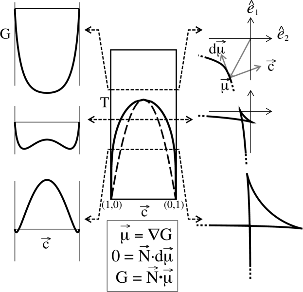
Figure 1: In the left column molar free energies for the regular solution model at temperatures $1.1T_{crit}$, $0.8T_{crit}$, $0.5T_{crit}$ are plotted. The chemical potentials at corresponding temperatures are plotted on the right; these curves trace out the ”$\vec{\mu}$-shapes.” The phase diagram is plotted for reference in the center. The crossings in the $\vec{\mu}$-shapes represent of two-phase equilibria. The compositions $\vec{c}$ are given by the normals to curve $\vec{\mu}$ and the two compositions in equilibrium at the crossing are also the common tangent points which could be drawn on $G(\mbox{$\vec{c}$})$. The ears represent metastable and unstable compositions; the sharp points on the ears are the spinodal points which are represented by dashed lines on the phase diagram, or points of inflection on $G(\mbox{$\vec{c}$})$.

Chemical potentials for both components can be obtained for this model by any one of a number of equivalent ways, e.g. by taking the derivatives of $\mbox{$G(\mbox{$\vec{N}$})$}=(N_{1}+N_{2})\mbox{$G(\mbox{$\vec{c}$})$}$ with respect to $N_{1}$ and $N_{2}$. Another is taking the intercepts at $c=0$ and $c=1$ of tangents at $c$ to $G_{m}(c)$. The resulting chemical potentials are plotted against each other in the figures of the right column of Figure 1. Since the coordinates of any point of this curve give the values of the two chemical potentials, these point are the ends of $\vec{\mu}$ is the gradient of $G(\mbox{$\vec{N}$})$. We wish to focus on this $\vec{\mu}$-shape.

At high $T$ this shape is smoothly curved. Because of the geometric relation in Equation 3 i.e., the Gibbs-Duhem equation in the case of solution thermodynamics, $\mbox{$\vec{c}$}\cdot d\mbox{$\vec{\mu}$}=0$, the normal to the $\vec{\mu}$ curve is the composition vector $\vec{c}$. Thus we can know the composition for each part of the curve. Once that is known we can recover $G(\mbox{$\vec{c}$})$ from this curve from $\mbox{$G(\mbox{$\vec{c}$})$}=\mbox{$\vec{c}$}\cdot\mbox{$\vec{\mu}$}$, but there are other ways.

Below the critical temperature the $\vec{\mu}$-plot becomes self-intersecting and develops ‘swallow-tails’ or ‘ears.’ The crossings are places where two phases (smooth curves) have the same chemical potential. Because of the Gibbs-Duhem equation relating slope to composition, the distinct compositions of each of the phases are given by the normals to the curve at the crossing point. The sharpness the corner at the crossing relates to the difference in composition between the two phases in equilibrium, i.e., the width of the miscibility gap in the phase diagram. This analogy between corners in $\vec{\mu}$-shapes and phase diagrams extends to multicomponent phase equilibrium.

The locally convex portions of the ears represent metastable compositions; the concave parts unstable compositions. The metastable and unstable part are separated by a spinode. Eliminating the ears produces a convex figure that is the convexified $\vec{\mu}$-shape. It contains all the information that was in the convexified $G(\mbox{$\vec{c}$})$ plus a graphic display of all the phase equilibria. This diagram illustrates the geometric nature of Equation 3.

The diagrams on the left and right side of Figure 1 are dual to each other. Each can be used to calculate the phase diagram in the center and any diagram on the right side ($G(\mbox{$\vec{c}$})$) can be used to calculate its dual $\vec{\mu}$-shape which appears on the right side of Figure 1. Note that even though the phase diagram cannot be used to determine any of the other figures uniquely, the special CALPHAD procedures have had considerable successes.[53, 6]

4.2 $\vec{\xi}$-plots

To draw out the analogy to the above discussion of binary phase diagrams, we consider an example of a two dimensional crystal. Discussion of three dimensional crystals can be found elsewhere[54].

A parallel geometric construction is made for an orientation dependent surface tension ($\mbox{$\gamma(\mbox{$\vec{n}$})$}=1+\alpha n_{1}^{2}n_{2}^{2}$) in Figure 2. This particular example is a first order expansion of a $\gamma(\mbox{$\vec{n}$})$ with square symmetry. It could also be written as $\gamma(\theta)=1+\alpha(Cos^{2}(\theta)Sin^{2}(\theta)$. The figure is remarkably similar to the construction for $G(\mbox{$\vec{N}$})$ in Figure 1 except that the figures are closed curves since the range of $\vec{A}$ is all of $R^{2}$

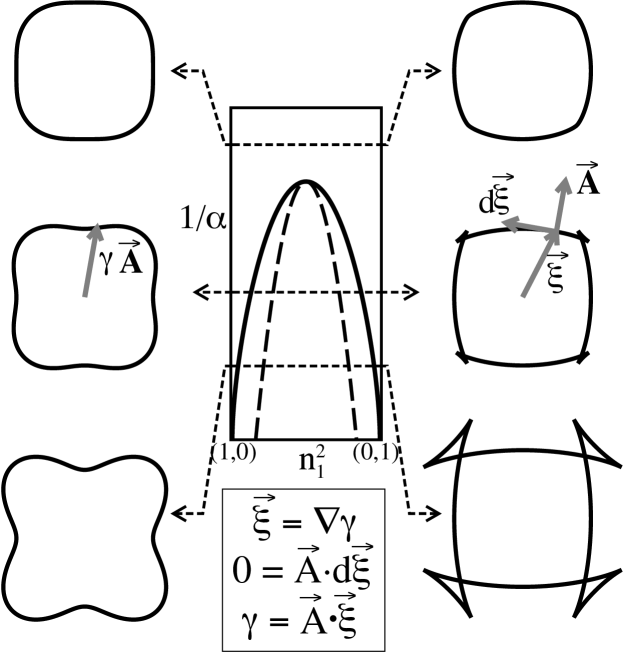
Figure 2: An analogous construction to that in Fig. 1 for an anisotropic $\gamma(\mbox{$\vec{n}$})$ for various values of an anisotropy parameter $\alpha$ (see text). In the left column $\gamma(\mbox{$\vec{n}$})$ is plotted from top to bottom for $\alpha=1/2$, 1, 2. Anisotropy increases with positive $\alpha$, so $1/\alpha$ is used in the $n$-diagram to correspond to the temperature axis in Fig. 1. The shape resulting from the gradient construction–with the ears removed–is the surface of the Wulff shape.

Increasing values of $\alpha$ increase the anisotropy in $\gamma(\mbox{$\vec{n}$})$ and tends to create higher energy orientations which disappear from the equilibrium shape. Thus, $1/\alpha$ plays a similar role to temperature, T, on the construction for the regular solution $G(\mbox{$\vec{c}$})$ and so $1/\alpha$ is the ordinate for the $n$-diagram illustrated in the center of Figure 2. The critical value of alpha is 4/7. Also, note that we use $n_{1}^{2}=Cos^{2}(\theta)$ as the ordinate which is convenient for this case of square symmetry.

Plots of $\gamma(\mbox{$\vec{n}$})$ appear on the left side of Figure 2 for three different values of $1/\alpha$, one above and two below the critical anisotropy. The gradient construction shown on the right column of the figure show that ‘ears’ develop as the anisotropy increases just as in the case for lower temperatures in the gradient construction for $G(\mbox{$\vec{N}$})$. Any orientation on the ‘ears’ is unstable and will break up into orientations given by the crossing in the $\vec{\xi}$-plot. Those parts on the concave part of the ‘ears’ (outside the spinodes) are metastable.[40]

Consider the geometrical relations for the gradient construction in Figure 2. According to Equation 2 (for surface energies, these are the Cahn-Hoffman equations [46, 47] $0=\mbox{$\vec{A}$}\cdot d\mbox{$\vec{\xi}$}$) the unit normal to the surface $\vec{\xi}$ must be the orientation vector. Therefore, for all stable orientations, the surface of $\vec{\xi}$ must also be the surface of the Wulff shape. In this sense, the interior region of the $\vec{\xi}$-plot must be equivalent to that obtained by the Wulff construction (See below).

4.3 Growth Shapes and Method of Characteristics

The method of characteristics has been used to integrate the first order partial differential equations that are obtained for the motion of a surface (or a growth front) when the velocity is a known function of the surface orientation $v(\mbox{$\vec{n}$})$. A thorough description may be found in Taylor and coworkers[32, 36] and applications may be found in Carter and Handwerker[55].

Let $\tau(\mbox{$\vec{x}$})$ be the arrival time of the surface at the position $\vec{x}$. The level set $\tau(\mbox{$\vec{x}$})=t_{const}$ is the equation for the position (or shape) of the surface at time $t=t_{const}$. The gradient of $\tau$ is along the normal of the level set and its magnitude must be inversely proportional to the velocity: $\|\nabla\tau\|=1/\mbox{$v(\mbox{$\vec{n}$})$}$. With $\mbox{$\vec{p}$}\equiv\nabla\tau$, the PDE is just a statement that the HD1 function $v$ is a constant: $v(\mbox{$\vec{p}$})=1$. The characteristics are straight lines, given by the equation:

$$\mbox{$\vec{x}$}=\mbox{$\vec{x}$}_{O}+t\mbox{$\vec{\chi}$}(\mbox{$\vec{n}$})\;,\;\;\mbox{where}\;\mbox{$\vec{\chi}$}(\mbox{$\vec{n}$})=\mbox{$\vec{\chi}$}(\mbox{$\vec{p}$})=\nabla v(\mbox{$\vec{p}$})$$ (6)

and $\mbox{$\vec{x}$}_{O}$ is the surface at $t=0$.

Letting the initial surface $\mbox{$\vec{x}$}_{O}$ be a point, the calculation of the shape at a fixed time (say t = 1) by the method of characteristics gives the same result as the gradient formulations.

5 Chemical Wulff Shapes

There is a large literature regarding the Wulff shape that minimizes surface energy for a given enclosed volume and the analogous kinetic Wulff shape that give the limiting shape of a crystal growing outwardly under diffusion control that has recently been reviewed.[32] The methods of construction are the same even though one is a minimization problem and the other is a long-time solution of a first-order nonlinear partial differential equation.

The method is one of iterative truncation of space by a set of half planes–each half plane partitions the space into allowed and disallowed half spaces. For each value of $\vec{n}$ a plane is drawn normal to $\vec{n}$ at a distance equal to the value of $\gamma(\mbox{$\vec{n}$})$ or $v(\mbox{$\vec{n}$})$ respectively and the half space of all the more distant points discarded. When this is done for all $\vec{n}$, the remaining points form a convex body that is the Wulff shape. The expression for the set of points which survive this construction is given by $\{\mbox{$\vec{x}$}|\mbox{$\vec{x}$}\cdot\mbox{$\vec{n}$}\leq\gamma(\mbox{$\vec{n}$})\;\forall\mbox{$\vec{n}$}\in S^{2}\}$ for $\gamma(\mbox{$\vec{n}$})$; substituting $v(\mbox{$\vec{n}$})$ for $\gamma(\mbox{$\vec{n}$})$ gives the kinetic Wulff shape.

The surface of the Wulff shape and the convexified $\xi$-plot or plot of the characteristics are the same shapes, even though they are obtained by quite different mathematical or graphical operations. In the Wulff constructions there is no restriction to either continuous or differentiable functions. Because no differentiation of date is used, the methods Wulff constructions may be quite superior for noisy data. Even though $G(\mbox{$\vec{c}$})$ is expected to be smooth for solutions it is worthwhile to propose a Wulff construction for solution and compound free energy data.

In order to do this we need to convert $G(\mbox{$\vec{c}$})$ into the Euclimolar free energy $G^{Eu}(c)=\mbox{$G(\mbox{$\vec{N}$})$}/\|N^{Eu}\|=\mbox{$G(\mbox{$\vec{c}$})$}/(\sum c^{2}_{i})^{1/2}$. For the binary regular solution example $G^{Eu}(c)=(c(1-c)+T(clnc+(1-c)ln(1-c)))/(1-2c-2c^{2})^{1/2}$. The left hand panel of figure 3 shows $G(\mbox{$\vec{c}$})$ for $T=0.45$ which is $0.9$ of the critical temperature, and therefore shows a miscibility gap. The second and third panels show $G^{Eu}(c)$, plotted respectively against $c$ and as a radial plot, for this same temperature. The third panel shows in addition one step in the Wulff construction for a single composition. A line for that composition is drawn perpendicular to another line from the origin with slope $tan^{-1}(c/1-c)$ and length $G^{Eu}(c)$; all points to the upper right of this line (shown gray) are discarded. Performing the Wulff construction on a finite set of $c$ results in a fan of truncation lines shown in the last panel. The clear area at the lower left is the chemical Wulff shape, whose envelope is the $\vec{\mu}$-plot. As with the $\vec{\mu}$-plot such a figure plots chemical potentials against each other, and compositions are obtained from slopes. It identifies single phases as continuous curves a two-phase equilibrium as the corner.

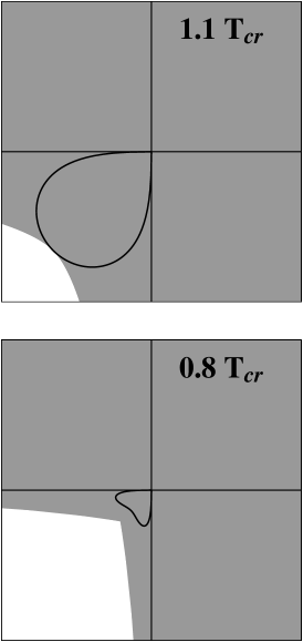
Figure 3: Illustration of the chemical Wulff construction. In the left figure, the molar free energy is plotted for a regular solution at $T=0.9T_{crit}$. In the middle two figures the Euclimolar free energy $G^{Eu}(c)$ (see text) for the same temperature is graphed as heavy curves in standard format and radially as $\mbox{$\vec{n}$}G^{Eu}(c)$. Note that the second and third plots look convex. In the third panel, one step in the chemical Wulff construction is illustrated. At a particular composition on $G^{Eu}$ a half plane is constructed which is normal to radius (thin black line) drawn from the origin. This divides the composition space into two parts: the gray region is to be discarded. In the final panel, the iterative elimination of discarded space yields the chemical Wulff shape.

The inverse Wulff construction, finding the distance of a tangent line from the origin corresponding to a particular composition recovers the Euclimolar free energy. Note that this is equivalent to $\mbox{$G(\mbox{$\vec{N}$})$}=\mbox{$\vec{\mu}$}\cdot\mbox{$\vec{N}$}$.

The concavity in the first panel of Fig. 3 shows that $G(\mbox{$\vec{N}$})$ at this $T$ is not convex. The corner in the Wulff construction in the last panel confirms this. Both are appropriate criteria for nonconvexity of $G(\mbox{$\vec{N}$})$. The convexity of the curves in the middle two panels is of Fig. 3 are of no importance; even though $G(\mbox{$\vec{N}$})$ is not convex, both curves are convex. For $\gamma(\mbox{$\vec{n}$})$ Herring’s tangent sphere construction for finding stable orientation is an alternate test for convexity. But this construction works only for positive functions. As can be seen in the third panel, it does not work for a radial plot of a negative $G^{Eu}(\mbox{$\vec{c}$})$.

Note that the two-phase corner does not touch the Euclimolar free energy plot; the gap is a measure of the reduction in free energy upon phase separation. The chemical Wulff shape does not give metastable phases or their equilibria, except when the entire curve of a stable phase is ignored in the construction. The undiscarded points in the interior of the lower left-hand area are not physically realizable, except possibly as an unknown stabler phase–an ice-9.[56]

Examples of the chemical Wulff construction for the three temperatures in Fig. 1 are illustrated in Fig. 4. They show not only the miscibility gaps at the lower temperature, but also the chemical potentials of the phases at various compositions derived from the normals. Note that in Fig. 4 that the Euclimolar free energy takes on some positive values as the temperature is decreased.

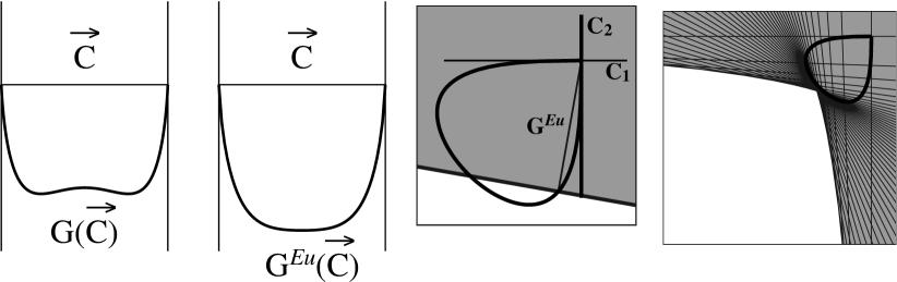
Figure 4: Illustration of the chemical Wulff construction for the three temperatures which were used in 1. The borders of the Wulff shapes are the same as the $\vec{\mu}$-shapes without ears.

6 Discussion

Analogies Between Phase Equilibria and Shape Morphology
	Composition Equilibrium	Surface Energy	Growth Shape
Convex	$G(\mbox{$\vec{N}$})$ at Const. $P$ and $T$	$\gamma(\mbox{$\vec{A}$})$ at Const. $\vec{\mu}$ and $T$	$v(\mbox{$\vec{p}$})$
Function
Common Tangent	$G(\mbox{$\vec{c}$})$	$1/\mbox{$\gamma(\mbox{$\vec{n}$})$}$	$1/\mbox{$v(\mbox{$\vec{n}$})$}$
Construction
Gradient	$\mbox{$\vec{\mu}$}(\mbox{$\vec{c}$})\equiv\nabla\mbox{$G(\mbox{$\vec{N}$})$}$	$\mbox{$\vec{\xi}$}(\mbox{$\vec{n}$})\equiv\nabla\mbox{$\gamma(\mbox{$\vec{A}$})$}$	$\mbox{$\vec{\chi}$}(\mbox{$\vec{n}$})\equiv\nabla\mbox{$v(\mbox{$\vec{p}$})$}$
Formulation
Geometric	$\mbox{$\vec{N}$}\cdot d\mbox{$\vec{\mu}$}=0$	$\mbox{$\vec{A}$}\cdot d\mbox{$\vec{\xi}$}=0$	$\mbox{$\vec{p}$}\cdot d\mbox{$\vec{\chi}$}=0$
Relations
Wulff	$\{\mbox{$\vec{\mu}$}|\mbox{$\vec{c}$}\cdot\mbox{$\vec{\mu}$}\leq G^{Eu}(\mbox{$\vec{c}$})\;\forall\mbox{$\vec{c}$}\in\Sigma_{+}^{\nu-1}\}$	$\{\mbox{$\vec{x}$}|\mbox{$\vec{x}$}\cdot\mbox{$\vec{n}$}\leq\gamma(\mbox{$\vec{n}$})\;\forall\mbox{$\vec{n}$}\in S^{2}\}$	$\{\mbox{$\vec{p}$}|\mbox{$\vec{p}$}\cdot\mbox{$\vec{n}$}\leq v(\mbox{$\vec{n}$})\;\forall\mbox{$\vec{n}$}\in S^{2}\}$
Construction

In this paper we have examined how the three topics to which Hubert Aaronson has contributes so much, phase equilibria, shape equilibria, and limiting shapes obtained with interface controlled growth, share a common mathematical basis, which is that in each case there are HD1 functions that are to be convexified. Because these topics have had separate developments, there are many methods that have been found useful in some but not all of the topics. These fall broadly into three areas as summarized in Table 1:

1. Those that operate on sub-manifolds of the HD1 function, such as $G(\mbox{$\vec{c}$})$, $\gamma(\mbox{$\vec{n}$})$, and $v(\mbox{$\vec{n}$})$, and use such methods as finding its common tangents and curvatures to give phase and shape diagrams, as well as limits of metastability. Here the choice of metric plays a role in deciding which plot is to be convexified; and two choices for $\gamma(\mbox{$\vec{n}$})$ are contrasted below. The shape or $n$-diagrams are simple analogs of phase diagrams with the missing orientations at edges and corners represented as two and multi-phase regions, and coexistent orientations represented by tie lines, triangles, etc.

2. Those that operate on the gradient of the HD1 function, the $\vec{\mu}$ and $\vec{\xi}$ plots and the characteristics to obtain shapes that have ready physical interpretation for $\gamma$ and $v$. Because of the Gibbs-Duhem relation the normals to any point on the $\mu$ plot gives its composition. The surfaces of the innermost parts of this plot represent equilibrium single phases and their composition ranges. Intersections to give edges and corners represent phases that are in equilibrium with one another. The missing orientations at edges and corners in this plot represent the composition gaps in the phase diagrams, and limiting orientations at these edges and corners.

   For the $\vec{\mu}$ and $\vec{\xi}$ plots the locally convex surfaces of the “ears” beyond these intersection represent metastable phases or surfaces; all other parts of the ears are separated from the metastable parts by spinodes and represent unstable phases or surfaces.

   There is no clear cut stability criterion for the characteristics; any characteristics can be stable at some time during shape evolution with arbitrary initial data. However the limiting shape of an outward growing crystal is the innermost plot, i.e. the plot without the ears.

3. Those that use a sub-manifold of the HD1 function in a graphical construction to obtain a shape that for $\gamma(\mbox{$\vec{n}$})$ and $v(\mbox{$\vec{n}$})$ is the Wulff shape. For $\gamma(\mbox{$\vec{n}$})$ this is the shape with the lowest surface energy for the volume it contains; for $v(\mbox{$\vec{n}$})$ this is the shape that for a given volume would add the least volume by further growth; it is also the limiting shape for outward growth. Such a construction can be done for $G(\mbox{$\vec{c}$})$, but the construction has to be modified because of the Manhattan metric for $\vec{N}$; this is awkward. If we convert $G(\mbox{$\vec{c}$})$ to a Euclimolar free energy, defined above, the unmodified Wulff construction works to give a $\vec{\mu}$-shape with equilibria alone.

The common mathematical basis has indeed made it possible to examine the analogies for all three topics and for all three basic methods. The differences in methods, such as common tangents on radial plots of $G(\mbox{$\vec{c}$})$ versus $1/\mbox{$\gamma(\mbox{$\vec{n}$})$}$, were often the result of the differences in the metrics in conventional use. Manhattan metrics work with the function; Euclidian metrics with the reciprocal. If we use a weighted metric for $\gamma$, such as energy/(unit area) projected along an axis, $\gamma^{m}$, the tangent constructions are done on this rather than its reciprocal. This metric is already in use for vicinal surfaces. Molar and molal free energies are convexified directly with equivalent results. The standard Wulff construction works with the Euclidian metric, and neither molar or molal free energies are easily used. But with the definition of a Euclimolar free energy we can directly create a $\vec{\mu}$ graphically, without taking derivatives of $G(\mbox{$\vec{c}$})$ or $G(\mbox{$\vec{N}$})$.

The analogies create many approaches for solving problems in all three topics. The advantages of having such flexibility in approach need to be explored. [44]

Phase diagram data are easy to obtain experimentally and can be obtained without knowing the free energy. Such data can be extrapolated. The topology of phase changes is guided by the phase rule; such phase changes appear on phase diagrams in standard formats. The same holds true for $n$-diagrams; the orientation of smooth surfaces and the orientation gaps at edges and corners which develop at local equilibrium, i.e., without waiting for full shape equilibration or without measuring $\gamma(\mbox{$\vec{n}$})$. From such data the $n$-diagrams can be constructed and extrapolated, identifying surface “phase changes” that conform to a phase rule that is modified for crystal symmetry. We have in an example [54] exploited this interconversion between shapes and phase equilibria to analyze a complex series of phase changes in a ternary regular solution.

All the information that is in $G(\mbox{$\vec{N}$})$ is not only in $G(\mbox{$\vec{c}$})$, but also in the $\vec{\mu}$ plots; the free energies can be recovered from such a plot. The same interconversion holds for the chemical Wulff plots and the convexified free energies. These plots all display the same information, but in different formats. Furthermore some plots are more sensitive to errors in the data because differentiation or finding the point of tangency is involved. Which plot is best will be partially determined by the nature of the data; chemical potential data ought to go directly into constructing a $\vec{\mu}$-plot. Free energy plots show free energy and composition, but coexistent compositions must be determined by a tangent construction that is very sensitive to errors in the data and becomes increasingly difficult with increasing number of components. The Wulff shape is obtained without differentiating the free energy data; the $\vec{\mu}$ shape requires taking a gradient of $G(\mbox{$\vec{N}$})$. These two plots should be congruent for the stable equilibria. They display phase coexistence clearly as corners and edges, compositions as normal directions, which implicitly requires differentiation, and free energy of a particular composition as the distance (in the appropriate metric) of the corresponding tangent plane from the origin.

The analogies are not perfect, as a few examples will show. The stability criteria are different for the kinetics. Curved surfaces can be part of the Wulff shape, and thus of an equilibrium shape. Only points in the $\vec{\mu}$-shape represent equilibria. Curved surfaces in this shape are ranges in the $\vec{\mu}$ and in the compositions. A system that spans such a range is not in equilibrium and has real- space gradients of the chemical potential. While there is a clear analogy with edges and corners, there appear to be no chemical analogy to a triple junction of surfaces.

7 Summary

In this paper, we have tied three fields together with a common mathematics based on the fact that the underlying extensive function must be convex. From such a common basis, gradient constructions are derived which have useful geometrical interpretations and allow results from one field to be applied through analogy to the others.

Apparent differences in the way common tangents are applied to compositions and to interfaces are resolved by consideration of the particular metric in use.

The analogies lead to the notion of the chemical Wulff shape which is constructed on chemical free energy normalized by the same euclidian metric which is used to normalize surface tension. This construction suggests a promising means to determine phase boundaries without resorting to numerical differentiation.

Finally, the common mathematical structure presents a unified way of studying, teaching, and understanding three important topics in materials science.

8 Acknowledgements

This work was supported by the NIST Materials Science and Engineering Laboratory, Ceramics Division, and the Center for Theoretical and Computational Materials Science. We appreciate useful discussions with A. Roosen, J. Blendell, J. Warren, R. Braun, J. Taylor, C. Handwerker and Hub Aaronson. We are also grateful to contribute to this acknowledgement of Hub Aaronson’s lasting contributions to our field.

References

- [1] V.F. Zackay and H.I. Aaronson, editors. Decomposition of Austenite by Diffusional Processes, NY, 1962. Interscience.
- [2] H.I. Aaronson. Lectures in the Theory of Phase Transformations. The Metallurgical Society, 1975.
- [3] R.F. Sekerka H.I. Aaronson, D.E. Laughlin and C.M. Wayman, editors. International Conference on Solid Solid Phase Transformations. The Metallurgical Society, 1982.
- [4] C. Laird H.I. Aaronson and K.R. Kinsman. Mechanisms of diffusional growth of precipitate crystals. American Society of Metals, page 313, 1970.
- [5] J.E. Hilliard D. Turnbull, J.S. Kirkaldy and H.I. Aaronson. On the teaching of a graduate course in phase transformations. Journal of Metals, 27(9):24–29, 1975.
- [6] J.K. Lee G.J. Shiflet and H.I. Aaronson. Application of the kaufman approach to the calculation of intra-rare earth phase diagrams. CALPHAD, 3(2):129–135, 1979.
- [7] H.I. Aaronson K.B. Alexander, F.K. LeGoues and D.E. Laughlin. On representation of the GP zone solvus in Al-Ag alloys. Scripta Met., 22:1671–1672, 1988.
- [8] H.A. Domian H.I. Aaronson and G.M. Pound. Thermodynamics of the austenite proeutectoid ferrite transformation. i, Fe-C alloys. Trans. A.I.M.E, 236:753–767, 1966.
- [9] H.A. Domian H.I. Aaronson and G.M. Pound. Thermodynamics of the austenite proeutectoid ferrite transformation. ii, Fe-C-X Alloys. Trans. A.I.M.E, 236:768–781, 1966.
- [10] H.I. Aaronson and H.A. Domian. Partition of alloying elements between austenite and proeutectoid ferrite or bainite. Trans. A.I.M.E, 236:781–796, 1966.
- [11] J.R. Bradely G.J. Shiflet and H.I. Aaronson. A re-examination of the thermodynamics of the proeutectoid ferrite transformation in Fe-C alloys. Met. Trans., 9A:999–1008, 1978.
- [12] J.K. Lee and H.I. Aaronson. Application of the modified Gibbs-Wulff construction to some problems in the equilibrium shape of crystals at grain boundaries. Scripta Met., 8:1451, 1974.
- [13] J.K. Lee and H.I. Aaronson. The equilibrium shape of a particle at macroscopic steps and kinks and the Gibbs-Wulff construction. Surface Science, 47:692–696, 1975.
- [14] H.I. Aaronson and J.K. Lee. The kinetic equations of solid-solid nucleation theory, ’lectures in the theory of phase transformations’. The Met. Soc. of AIME, New York, pages 83–115, 1975.
- [15] J.K. Lee and H.I. Aaronson. Influence of faceting upon the equilibrium shape of nuclei at grain boundaries. i, two dimensions. Acta Met., 23:799–808, 1975.
- [16] J.K. Lee and H.I. Aaronson. Influence of faceting upon the equilibrium shape of nuclei at grain boundaries. ii, three-dimensions. Acta Met., 23:809–820, 1975.
- [17] H.I. Aaronson J.K. Lee and K.C. Russell. On the equilibrium shape for a non-centro-symmetric -plot. Surface Science, 51:302–304, 1975.
- [18] D.E. Graham S.P. Clough C.L. White J.K. Lee, D.W. Dooley and H.I. Aaronson. Two families of analytic -plots and their influence upon homogeneous nucleation kinetics. Surface Science, 62:695–706, 1977.
- [19] H.I. Aaronson G.J. Shiflet and T.H. Courtney. Kinetics of the approach to equilibrium shape of a disc-shaped precipitate. Scripta Met., 11:677–680, 1977.
- [20] G.J. Shiflet K.C. Russell Kwai S. Chan, J.K. Lee and H.I. Aaronson. Generalization ofthe nucleus shape-dependent parameters in the nucleation rate equation. Met. Trans., 9A:1016–1017, 1978.
- [21] J.K. Lee R.V. Ramanujan and H.I. Aaronson. A discrete lattice plane analysis of the interfacial energy of coherent fcc:hcp interfaces and its application to the nucleation of ’ in Al-Ag alloys. Acta Met., 40:3421–3432, 1992.
- [22] M.R. Plichta and H. Aaronson, editors. The Massive Transformation. Met. Trans., 1984.
- [23] H.I. Aaronson. On the growth mechanism of sideplates. Acta Met., 11:219–223, 1963.
- [24] C. Laird and H.I. Aaronson. Mechanisms of formation of and dissolution of ’ precipitates in an Al-4 Acta Met., 14:171–185, 1966.
- [25] H.I. Aaronson and H.B. Aaron. The initial stages of the cellular reaction. Met. Trans., 3:2743–2756, 1972.
- [26] J. Willard Gibbs. On the equilibrium of heterogeneous substances (1876). In Collected Works, volume 1. Longmans, Green, and Co., 1928.
- [27] J.C. Baker and J.W. Cahn. The thermodynamics of solidification. ASM Seminar Series on ‘Solidification’, pages 23–58, 1971.
- [28] F. C. Frank. The geometrical thermodynamics of surfaces, pages 1–15. American Society for Metals, 1963.
- [29] J. W. Cahn. Transitions and phase equilibria among grain boundary structures. J. de Physique, 43(C6):199–213, 1975. Also, Proceedings of Conference on the Structure of Grain Boundaries, Caen, France.
- [30] Conyers Herring. Some theorems on the free energies of crystal surfaces. Phys. Rev., 82(1):87–93, 1951.
- [31] H.I. Aaronson and K.R. Kinsman. Growth mechanisms of precipitate crystals. Trans. A.C.A., 1:25, 1971.
- [32] Jean E. Taylor, John W. Cahn, and Carol A. Handwerker. Geometric models of crystal growth (Overview no. 98-1). Acta Met., 40:1443–1474, 1992.
- [33] H.I. Aaronson. Atomic mechanisms of diffusional nucleation and growth and comparisons with their counterparts in shear transformations. Met. Trans. A, 24(2):241–276, 1993. 1990 Inst. of Metals Lecture.
- [34] H.I. Aaronson and Y.C. Liu. On the turnbull and the cahn theories of the cellular reaction. Scripta Met., 2:1, 1968.
- [35] J. D. Livingston and J. W. Cahn. Discontinous coarsening of aligned eutectoids. Acta Met., 22:495–503, 1974.
- [36] J. E. Taylor J. W. Cahn and C. A. Handwerker. Evolving crystal forms: Frank’s characteristics revisited. In A Keller A. R. Lang R G Chambers, J E Enderby and J W Steeds, editors, Sir Charles Frank, OBE, FRS, An eightieth birthday tribute, pages 88–118, New York, 1991. Adam Hilger.
- [37] C.A. Handwerker J.E. Blendell Y.J. Baik D.Y. Yoon, J.W. Cahn. In Interface Migration and Control of Microstructure, Metals Park, Ohio, 1986. ASM Press.
- [38] C.A. Handwerker. In Diffusion Phenomena in Thin Films and Microelectronic Materials, pages 245–332, Park Ridge, New Jersey, 1988. Noyes.
- [39] I.M. Gelfand and S.V. Fomin. Calculus of Variations. Prentice-Hall, Inc., Englewood Cliffs, New Jersey, 1963.
- [40] William W. Mullins. Solid surface morphologies governed by capillarity. In Metal Surfaces, pages 17–66. American Society for Metals, 1963.
- [41] Jean E. Taylor. Crystalline variational problems. Bull. AMS, 84:568–588, 1978.
- [42] E. Arbel and J. W. Cahn. On invariances in surface thermodynamic properties and their applications to low symmetry crystals. Surface Science, 51:305–309, 1975.
- [43] J.E. Taylor. Mean curvature and weighted mean curvature, overview 98(ii). Acta Met., 40(7):1475–1485, 1992.
- [44] W.C. Carter and J.W. Cahn. The morphology of corners, edges and facets and the thermodynamics of phase stability useful insights by direct analogy. Acta Met. in preparation.
- [45] Kenneth Denbigh. The Principles of Chemical Equilibrium. Cambridge University Press, London, 1971.
- [46] David W. Hoffman and John W. Cahn. A vector thermodynamics for anisotropic surfaces. i. fundamentals and applications to plane surface junctions. Surface Science, 31:368–388, 1972.
- [47] J. W. Cahn and D. W. Hoffman. A vector thermodynamics for anisotropic surfaces. ii. curved and facetted surfaces. Acta Met., 22:1205–1214, 1974.
- [48] F. C. Frank. On the kinematic theory of crystal growth and dissolution processes. In Growth and Perfection of Crystals, pages 411–419. John Wiley, New York, 1958.
- [49] F. C. Frank. Z. f. Physik. Chemie N.F., 77:84–92, 1972.
- [50] J.W. Cahn and F. Larche. A simple model for coherent equilibrium. Acta Met., 32(11):1915–1923, 1984.
- [51] A.F. Andreev. Faceting phase transisitions of crystals. Sov. Phys. JETP, 53(5):1063–1069, 1981.
- [52] L.D Landau and E.M. Lifshitz. Statistical Physics. Pergammon Press, New York, 1963.
- [53] G.M. Pound S. Kaufman and H.I. Aaronson. Nucleation sites of bainitic carbides in alloy steels. Trans. A.I.M.E, 209:885, 1957.
- [54] W.C. Carter and J.W. Cahn. Directs analogies between shape morphology and phase transitions in ternary systems. Acta Met. in preparation.
- [55] W. Craig Carter and Carol A. Handwerker. Morphology of grain growth in response to diffusion induced elastic stresses: Cubic systems. Acta Met., 41(5):1633–1642, 1993.
- [56] Kurt Vonnegut Jr. Cat’s Cradle. Dell Publishing Co, New York, 1963. pp 38-39.