Exact low temperature results for transport properties of the interacting resonant level model

Abstract

Using conformal field theory and integrability ideas, we give a full characterization of the low temperature regime of the anisotropic interacting resonant level (IRLM) model. We determine the low temperature corrections to the linear conductance exactly up to the 6th order. We show that the structure displays ’Coulomb deblocking’ at resonance, i.e., a strong impurity-wire capacitive coupling enhances the conductance at low temperature.

Transport properties in quantum impurity problems have become central to experimental nanophysics rev . Their theoretical study involves strong interactions, often out of equilibrium, and thus presents considerable difficulties. In many cases, it is possible to map these systems to simple one dimensional models, which can be solved by the Bethe ansatz (BA) in equilibrium. Extending the BA out of equilibrium is the next step forward. This has been accomplished in the problem of edge state tunneling in the fractional quantum Hall effect (where coupling to the reservoirs was particularly simple) FLS ,BLZ , but major obstacles remain in most other cases KLS . Recently, an exciting new “open Bethe ansatz” has been proposed Natan , which might well be a breakthrough, although subtle issues remain open - related to universality and the treatment of boundary conditions around the impurity out of equilibrium: see Benjamin for recent progress in this direction.

It is one of the major difficulties of this field that so few methods are available to investigate strongly correlated regimes that it is often not possible to assert the validity of results such as those in FLS or Natan (see eg Borda ). Our goal in this paper is to report on a method to tackle low temperature properties in the IRLM which gives highly non perturbative results, and apart from its own usefulness, provides results that can be used as benchmarks. Another, different perturbative approach has been proposed recently in Benjamin .

The IRLM model describes a resonant level coupled via tunneling junctions to two baths of spinless electrons, with which there is also a Coulomb interaction Natan ; Andrei . After the usual expansion in angular modes, unfolding and linearizing near the Fermi surface, one ends up with a hamiltonian $H=H_{0}+H_{B}$ where $H_{0}=-i\sum_{a=1,2}\int dx\,\psi^{\dagger}_{a}\partial_{x}\psi_{a}$ is the free hamiltonian describing two infinite right moving Fermi wires, and tunneling occurs through the impurity term:

$$\begin{array}[]{c}H_{B}=\left(\gamma_{1}\psi_{1}(0)+\gamma_{2}\psi_{2}(0)\right)\,d^{\dagger}+\mbox{h.c.}\vspace{0.1cm}\\ +\;U\;\big{(}\psi^{\dagger}_{1}\psi_{1}(0)+\psi^{\dagger}_{2}\psi_{2}(0)\big{)}\,\big{(}d^{\dagger}d-\textstyle\frac{1}{2}\big{)}+\epsilon_{d}~{}d^{\dagger}d\end{array}$$ (1)

In the following, it will be convenient to use the langage of the Kondo model, which is unitarily related to the IRLM wiegmann78 , and to introduce spin $1/2$ operators to represent the impurity: $d^{\dagger}=\eta S^{+}$, $d^{\dagger}d=S^{z}+\frac{1}{2}$ ($\eta$ is a Majorana fermion). The parameters $\gamma_{1,2}$ (which can be taken real) are parametrized as $\gamma_{1}+i\gamma_{2}=\gamma\sqrt{2}e^{i\theta/2}$ ; $\theta$ encodes anisotropy in the tunneling process. Note the presence of the important interaction term, a capacitive coupling $U$ between the impurity and the wires. When the on-site chemical potential $\epsilon_{d}$ vanishes, the impurity is at resonance (in an actual experiment this would require adjusting the local grid potential to some value $V_{g}(U)$).

We shall be concerned with the conductance of the structure when a voltage $V$, that couples as $H_{V}=\sum_{a=1,2}\int dx\,(\psi^{\dagger}_{1}\psi_{1}-\psi^{\dagger}_{2}\psi_{2})$, is applied across the impurity. The standard approach to this model is to form the combinations $\psi_{+/-}=\frac{1}{\gamma\sqrt{2}}\big{(}\gamma_{1/2}\psi_{1}\pm\gamma_{2/1}\psi_{2}\big{)}$, which lead to decoupling into two independent sectors, where $H$ can be diagonalized using a straightforward BA Wiegmann . Using Friedel’s sum rule the linear conductance $G={dI\over dV}\big{|}_{V=0}$ is given at temperature $T=0$ by:

$$G_{\tiny\mbox{IR}}=\textstyle{\frac{e^{2}}{h}}\;\sin^{2}\theta\;\sin^{2}(\pi n_{d})$$ (2)

The term $\sin^{2}\theta=\frac{2\gamma_{1}\gamma_{2}}{\gamma_{1}^{2}+\gamma_{2}^{2}}$ is the familiar tunneling anisotropy prefactor ; the impurity filling $n_{d}=\left\langle d^{\dagger}d\right\rangle$ can be extracted in ’closed form’ at zero temperature using BA in the $\psi_{\pm}$ basis ponomarenko93 . However, going beyond formula (2), which is valid only at $V=T=0$ is a very difficult task within this BA. The problem is that one is typically interested in situations where the two wires are at different chemical potentials, an ensemble very difficult to represent in the $\psi_{\pm}$ basis. We will show in this paper that in the field theory limit, several important results can nevertheless be obtained by exploiting hidden symmetries. We will present the boundary conditions characterizing the zero temperature or infrared (IR) fixed point by making use of an underlying SU(2) structure. This gives an alternative, straightforward way to obtain the IR conductance (2) but also allows for the setting up of a convenient formalism (perturbed boundary conformal field theory) for systematically obtaining the low $T$ corrections to conductance (formulae (14,15)).

Our results rely on two equivalent representations of (1) in the field theory limit. We will initially set the on-site chemical potential $\epsilon_{d}=0$, but reinstate it later. First, let us bosonize $\psi_{\pm}=\frac{\eta_{\pm}}{\sqrt{2\pi}}\,e^{i\sqrt{4\pi}\varphi_{\pm}}$. This yields

$$\begin{array}[]{ccc}H\!&=&\!\sum_{a=\pm}H_{0}(\varphi_{a})+\frac{\gamma\kappa^{+}}{\sqrt{\pi}}\,\big{[}e^{i\sqrt{4\pi}\varphi_{+}}(0)\,S^{+}+\mbox{h.c.}\big{]}\vspace*{0.1cm}\\ &&\hskip 14.22636pt+\frac{U}{\sqrt{\pi}}\,\left(\partial_{x}\varphi_{+}(0)+\partial_{x}\varphi_{-}(0)\right)\,S^{z}\end{array}$$ (3)

where the free hamiltonian is $H_{0}(\varphi_{a})=\frac{1}{2}\int dx\,\left(\partial_{x}\varphi_{a}\right)^{2}$ and $\kappa^{+}=\eta\eta_{+}$. We then perform the unitary transformation ${\cal U}=e^{i\alpha S^{z}\!\left(\varphi_{+}\!+\!\varphi_{-}\right)(0)}$ and choose $\alpha=\frac{U}{\sqrt{\pi}}$, to cancel the remaining interaction along $S^{z}$. Define now $\phi_{+}=\frac{1}{\beta}\big{[}(\sqrt{4\pi}\!-\!\alpha)\varphi_{+}\!-\!\alpha\varphi_{-}\big{]}$ and $\phi_{-}=\frac{1}{\beta}\big{[}(\sqrt{4\pi}\!-\!\alpha)\varphi_{-}\!+\!\alpha\varphi_{+}\big{]}$, with $\beta^{2}=\frac{2}{\pi}(U-\pi)^{2}+2\pi$. In terms of these new variables, the hamiltonian then becomes:

$$H^{I}=\sum_{a=\pm}H_{0}(\phi_{a})+\frac{\gamma\kappa_{+}}{\sqrt{\pi}}\,\left[e^{i\beta\phi_{+}}(0)\,S^{+}+\mbox{h.c.}\right]$$ (4)

A remarkable feature is that the angle $\theta$ has disappeared from this expression; as a result, the free energy of the impurity problem is independent of the anisotropy. Hamiltonian $H^{I}$ is formally equivalent to the anisotropic Kondo problem. The interaction term has scaling dimension $D=\frac{\beta^{2}}{8\pi}$ and thus we see immediately that in the scaling theory, tunneling is irrelevant in the low energy limit for $\beta^{2}>8\pi$ i.e. strong Coulomb interaction $|U-\pi|>\sqrt{3}\pi$ and relevant otherwise. In the latter case, the $\phi_{+}$ hamiltonian flows to the ordinary Kondo fixed point. We will soon argue this corresponds to the resonant level being hybridized with the wires, with a fixed, anisotropy dependent amount of tunneling between the two.

To proceed, observe that we could first bosonize $\psi_{1,2}$ and then only form linear combinations, this time of the bosons. Setting $\psi_{a}=\frac{\eta_{a}}{\sqrt{2\pi}}\,e^{i\sqrt{4\pi}\varphi_{a}}$ and forming the combinations $\phi_{1}=\frac{1}{\sqrt{2}}\left(\varphi_{1}+\varphi_{2}\right)$, $\phi_{2}=\frac{1}{\sqrt{2}}\left(\varphi_{1}-\varphi_{2}\right)$, the Hamiltonian is then rotated by the same unitary transformation ${\cal U}=e^{i\alpha\sqrt{2}\,S^{z}\,\phi_{1}(0)}$ to yield

$$H^{I\!\!I}=\sum_{a=1,2}H_{0}(\phi_{a})+\frac{\gamma}{\sqrt{2\pi}}\,\left[{\cal V}_{1}(0){\cal O}_{2}(0)S^{+}+\hbox{h.c.}\right]$$ (5)

where we have introduced the vertex operators ${\cal V}_{\pm 1}=e^{\pm i\beta_{1}\phi_{1}}$, ${\cal V}_{\pm 2}=e^{\pm i\sqrt{2\pi}\phi_{2}}$, ${\cal O}_{2}=\gamma_{1}\kappa_{1}{\cal V}_{2}+\gamma_{2}\kappa_{2}{\cal V}_{-2}$ and $\kappa_{a}=\eta\eta_{a}$. The parameter $\beta_{1}=\sqrt{2\pi}-\alpha\sqrt{2}$ satisfies $\beta^{2}=\beta^{2}_{1}+2\pi$ which ensures that the perturbations have the same scaling dimension $D$. This representation of the Hamiltonian is more suited to non equilibrium situation since the electrical current from wire 1 to 2 is simply expressible in terms of $\phi_{2}$ only. However, $H^{I\!\!I}$ has a much more complex form than $H^{I}$, and typically mixes Kondo and boundary sine-Gordon (BSG) type interactions. This is particular clear in the case $\beta_{1}\!=\!0$: in the limit $\theta\to 0$, the Hamiltonian reduces to $H_{B}^{I\!\!I}={\gamma\kappa_{1}\over\sqrt{\pi}}e^{i\sqrt{2\pi}\phi_{2}}S^{+}+\mbox{h.c.}$, a Kondo hamiltonian. If, for the sake of argument, we neglect the Klein factors (this is allowed for example in the computation of the free energy), the case $\gamma_{1}=\gamma_{2}$ reduces to $H_{B}^{I\!\!I}=4\gamma/\sqrt{2\pi}\cos(\sqrt{2\pi}\phi_{2})S^{y}$ i.e. two copies of the BSG model for $S^{y}=\pm{1\over 2}$. We will see later that indeed, reintroducing the Klein factors, the model at $\beta_{1}=0$ and $\gamma_{1}=\gamma_{2}$ shares the same (Dirichlet) boundary conditions with the BSG model.

That the free energy of the two incarnations $H^{I}$ and $H^{I\!\!I}$ is the same and independent of $\theta$ is remarkable. It can be checked directly but not straightforwardly at all order of the perturbative expansion in powers of $\gamma$.

We consider the question of the linear conductance at low energy, i.e. when the resonant level is hybridized with the wires. A quick way to obtain it is to use the boundary conditions (BC’s) for the fields $\phi_{1,2}$ in the IR. These are not so easy to obtain from hamiltonian $H^{I\!\!I}$. We will thus start from the BC’s for the fields $\phi_{\pm}$, which are known from the general analysis of the Kondo model. The idea is to follow these BC’s through the canonical transformations. This seems very hard due to the non linearities involved, but becomes possible once one recognizes the presence of SU(2) affine currents (the SU(2) transformations are those mixing the two wires). Introducing

$$\begin{array}[]{rclcrcl}J^{a}&=&\frac{1}{2}\,:\psi^{\dagger}_{\alpha}\sigma^{a}_{\alpha\beta}\psi_{\beta}:&\!,&J^{z}&=&\frac{1}{\sqrt{2\pi}}\,\partial_{x}\phi_{2},\\ &&&&&&\vspace{-0.25cm}\\ J^{x}&=&\frac{-i\rho}{2\pi}\sin(\sqrt{8\pi}\phi_{2})&\!,&\;J^{y}&=&\frac{-i\rho}{2\pi}\cos(\sqrt{8\pi}\phi_{2}),\end{array}$$ (6)

(here $\rho=\kappa_{1}\kappa_{2}$) it is easy to show that

$$\partial_{x}\phi_{-} = \textstyle{\frac{\sqrt{2\pi}}{\beta}}\;\partial_{x}\phi_{1}-\sqrt{2\pi}\textstyle{\frac{\beta_{1}}{\beta}}\left[\cos\theta J^{z}+\sin\theta J^{x}\right]$$

$$\partial_{x}\phi_{+} = \textstyle{\frac{\beta_{1}}{\beta}}\;\partial_{x}\phi_{1}+\textstyle{\frac{2\pi}{\beta}}\,\left[\cos\theta J^{z}+\sin\theta J^{x}\right]$$ (7)

We now recall that in the IR the field $\phi_{+}$ obeys Neumann BC’s with angle $\frac{\beta}{4}$, $\phi_{+}(0^{+})=\phi_{+}(0^{-})+{\beta\over 4}$, and the boson $\phi_{-}$ – being unaffected by the interaction – Neumann BC’s with angle $0$. Introducing SU(2) rotated currents $\tilde{J}^{a}={\cal R}^{y}_{\theta}\cdot J^{a}$ (${\cal R}_{\theta}^{y}$ is a rotation of angle $\theta$ around $J^{y}$), we see that in the IR, these currents obey the BC’s $\tilde{J}^{z}(0^{+})=J^{z}(0^{-})$ and $\tilde{J}^{\pm}(0^{+})=-\tilde{J}^{\pm}(0^{-})$. A little algebra based on the SU(2) commutation relations then leads to

$$J^{z}(0^{+}) = \cos(2\theta)\,J^{z}(0^{-})+\sin(2\theta)\,J^{x}(0^{-})$$

$$J^{x}(0^{+}) = -\cos(2\theta)\,J^{x}(0^{-})+\sin(2\theta)\,J^{z}(0^{-})$$

$$J^{y}(0^{+}) = -J^{y}(0^{-})$$ (8)

which of course are highly non linear in terms of the field $\phi_{2}$ itself. As for $\phi_{1}$, it obeys simply $\phi_{1}(0^{+})=\phi_{1}(0^{-})+{\beta_{1}\over 4}$. The BC’s for $\phi_{2}$ interpolate continuously between Neumann (N) ($\theta\!=\!0$ and $\phi_{2}(0^{+})\!=\!\phi_{2}(0^{-})\!+\!\sqrt{\pi/8}$) and double Dirichlet (D) ($\theta\!=\!\frac{\pi}{2}$ and $\phi_{2}(0^{+})\!=\!-\phi_{2}(0^{-})\!\pm\!\sqrt{\pi/8}$). This is possible because the dimension of the operator $e^{\pm i\sqrt{2\pi}\phi_{2}}$ is the inverse of an integer square, here $\frac{1}{2^{2}}$ strings . As a result, the ratio of boundary degeneracies for N and D is $g_{\mbox{\scriptsize N}}/g_{\mbox{\scriptsize D}}=2$, and degeneracies of N and double D are the same. That the two fixed points can be reached depending on $\theta$ is particular clear in the case $\beta_{1}=0$ discussed previously, where $H^{I\!\!I}$ interpolates between Kondo and double BSG. Independently of $\theta$, the IR boundary degeneracy thus always takes the N value, $g_{{\tiny\mbox{IR}}}=g_{\mbox{\scriptsize N}}$.

Another way of viewing these BC’s is to observe that the radius of compactification $r=\sqrt{2}$ being an integer multiple of the self dual radius $r^{*}=\frac{1}{\sqrt{2}}$ allows for the existence of a pair of non chiral operators of dimension one, $e^{\pm i\sqrt{2\pi}(\phi_{2}+\bar{\phi}_{2})}$, which induce an exactly marginal boundary deformation through $J^{x,y,z}$. To our knowledge, this is the first time such a BC is encountered in a condensed matter context. It is also the first time that a tunable flow into a line of boundary fixed points is encountered.

A similar analysis can be carried out when there is a chemical potential for the electron on the dot, i.e. a term $\epsilon_{d}d^{\dagger}d=\epsilon_{d}(S^{z}+\frac{1}{2})$. As before we first argue for the Kondo hamiltonian $H^{I}$. The local magnetic field results in an additional phase shift for the electrons Natanold , which translates into a phase shift $\delta_{+}$ for the field $\phi_{+}$. This is easy to understand: an additional phase shift for $\phi_{+}$ in the IR is tuned by the introduction of a scattering potential term, which then induces, by Friedel sum rule, an extra “charge” (here, magnetization) on the impurity. Now, it is known that the problem with a field acting on the impurity only is closely related Lowenstein (in the scaling limit) to the problem with a field coupling to the total spin $S_{tot}^{z}=S^{z}+{2\over\beta}\int\partial_{x}\phi_{+}$ which is immediately solvable by BA. This gives rise to the impurity magnetization $m_{imp}=\left\langle S^{z}\right\rangle=n_{d}-\frac{1}{2}$, with the relation $\delta_{+}=\sqrt{\pi\over 2}\;m_{imp}$. At $T=0$, the impurity magnetization can be obtained using the Wiener Hopf technique. One finds two possible expansions. For small enough $\epsilon_{d}$ one has

$$\vspace*{-0.1cm}m_{imp}={1\over D\sqrt{\pi}}\sum_{n=0}^{\infty}{(-1)^{n}\over n!(2n+1)}\frac{\Gamma\big{(}\frac{2n+1}{2(1-D)}\big{)}}{\Gamma\big{(}\frac{(2n+1)D}{2(1-D)}\big{)}}u^{2n+1}$$ (9)

with $u=\frac{D}{\sqrt{\pi}}\frac{\Gamma(D/2(1-D))}{\Gamma(1/2(1-D))}\frac{\epsilon_{d}}{T_{B}}$. The dual expression should be used beyond the radius of convergence $u^{*}=D^{\frac{D}{2(1-D)}}\sqrt{1\!-\!D}$:

$$\vspace*{-0.1cm}m_{imp}={1\over 2\sqrt{\pi}}\sum_{n=0}^{\infty}{(-1)^{n}\over n!}{\Gamma({1\over 2}\!+n(1-D))\over\Gamma(1-nD)}u^{2n(D-1)}$$ (10)

The parameter $T_{B}$ is the Kondo temperature for the problem defined by hamiltonian $H^{I}$, related to the bare coupling by $T_{B}/W=\frac{\Gamma(D/2(1-D))\Gamma(1-D)^{\frac{1}{1-D}}}{\sqrt{\pi}\;\;\Gamma(1/2(1-D))}\big{(}\frac{\gamma}{\sqrt{W}}\big{)}^{\frac{1}{1-D}}$, with $W$ the bandwidth (this relation holds within the regularization inherited from integrability used in Ref.LS ).

The additional phase shift for $\phi_{+}$ translates into more complicated non linear BC’s for the boson $\phi_{2}$: namely, the rotated currents $\tilde{J}^{a}$ now obey the BC’s $\tilde{J}^{z}(0^{+})=\tilde{J}^{z}(0^{-})$ and $\tilde{J}^{\pm}(0^{+})=-e^{\pm i\Delta}\tilde{J}^{\pm}(0^{-})$, with the angle $\Delta=2\pi m_{imp}$. After some calculations one finds

$$\begin{array}[]{l}J^{z}(0^{+})=\left[\cos^{2}\theta-\sin^{2}\theta\cos\Delta\right]J^{z}(0^{-})\vspace{0.1cm}\\ \hskip 17.07182pt+\sin(2\theta)\cos^{2}\frac{\Delta}{2}\;J^{x}(0^{-})+\sin\theta\sin\Delta\;J^{y}(0^{-})\hphantom{\hskip 18.49411pt}\vspace{0.2cm}\end{array}\vspace*{-0.65cm}$$

$$\begin{array}[]{l}J^{x}(0^{+})=\left[\sin^{2}\theta-\cos^{2}\theta\cos\Delta\right]J^{x}(0^{-})\vspace{0.1cm}\\ \hskip 17.07182pt+\sin(2\theta)\cos^{2}\frac{\Delta}{2}\;J^{z}(0^{-})-\cos\theta\sin\Delta\;J^{y}(0^{-})\vspace{0.2cm}\end{array}\vspace*{-0.65cm}$$ (11)

$$\begin{array}[]{l}J^{y}(0^{+})=-\sin\theta\sin\Delta\;J^{z}(0^{-})\vspace{0.1cm}\\ \hskip 17.07182pt+\cos\theta\sin\Delta\;J^{x}(0^{-})-\cos\Delta\;J^{y}(0^{-})\hphantom{\hskip 54.06006pt}\end{array}$$

These BC’s relate the currents on both sides of the impurity through a SU(2) rotation now depending on the anisotropy and doping of the impurity.

To extract information from the BC’s in the IR, it is convenient to reformulate them first within a boundary field theory by folding and introducing complex coordinates $z=\tau-ix$, $x>0$. The Kubo formula then reads:

$$G\!=\!\lim_{\omega\to 0}\frac{e^{2}}{\hbar}\frac{1}{(2L)^{2}}\frac{1}{\omega}\!\int\!dxdyd\tau e^{i\omega\tau}\left\langle j_{e}(x,\tau)j_{e}(y,0)\right\rangle$$ (12)

where $0<\tau<T^{-1}$, spacial integrals run over $[0,L]$ and $L$ has to be sent to $+\infty$; the electrical current through the whole structure is $j_{e}(x)=2\big{(}J^{z}(x)-J^{z}(-x)\big{)}$ (the conductance depends only on the $\phi_{2}$ propagator).

Using the propagators that can be deduced from (11):

$$4\pi\left\langle\partial_{x}\phi_{2}(z)\partial_{x}\phi_{2}(w)\right\rangle = \left(z-w\right)^{-2}$$ (13)

$$4\pi\left\langle\partial_{x}\phi_{2}(z)\partial_{x}\phi_{2}(w^{*})\right\rangle = \big{(}1-2\sin^{2}\theta\cos^{2}\!\textstyle\frac{\Delta}{2}\big{)}\left(z-w^{*}\right)^{-2}$$

one finds $G_{\tiny\mbox{IR}}=\frac{e^{2}}{h}\,\sin^{2}\theta\cos^{2}\frac{\Delta}{2}$, which is nothing but Eq.(2). The capacitive coupling $U$ has disappeared at the IR fixed point: it is ’irrelevant’, but as we will see, it controls the approach of the fixed point and thus determines the low $T<T_{B}$ properties of the theory, which we will now be able to tackle, thanks to this long reformulation of Friedel sum rule.

Indeed, the exact solution of the Kondo hamiltonian leads to a full knowledge of the infinity of counter-terms necessary to describe the approach to this fixed point LS , allowing one to carry out IR perturbation theory to all orders. A program such as the one of LSi could then lead to results for the linear conductance at arbitrary values of the temperature. It relies on the identification of the low $T$ Hamiltonian, which has the form: $H=H_{\tiny\mbox{IR}}+\sum_{k>0}b_{2k-1}{\cal O}_{2k}(x=0)$. It is important to stress that this expansion is highly non perturbative in the tunneling amplitude (as we will see below, it leads to an expansion of the conductance in powers of $\gamma^{-2/1-D}$). But the couplings $b_{2k-1}$ turn out to be known explicitly LSi ! The whole set of perturbing operators ${\cal O}_{2k}$ is a set of commuting conserved quantities related to integrability and describes the approach to the IR fixed point; it is made of fields of even dimensions. ${\cal O}_{2k}$ can be expressed as a polynomial in $\partial_{x}\phi_{+}$ and its derivatives, to be then translated in the $\phi_{1,2}$ basis. We just sketch here the (somewhat lenghty) analysis. Apart from density-density couplings, the leading irrelevant contribution contains a tunneling term ${\cal O}_{2}^{\mbox{\scriptsize tun}}=\lambda(\psi_{1}^{\dagger}\psi_{1}+\psi_{2}^{\dagger}\psi_{2})\big{(}\psi_{1}^{\dagger}\psi_{2}+\hbox{h.c.}\big{)}$ with a coupling constant $\lambda\propto{\beta_{1}\over\beta^{2}}\sin\theta$. The anisotropy and coulombic repulsion are only apparent in the amplitude of the tunneling term – which, as it should, vanishes in the Kondo limit, $\theta=0$. This pattern generalizes to all orders: the whole set of operators describing the approach to the IR fixed point is independent of $U$.

Figure 1: First three reduced coefficients $a_{2k}=g_{2k}(T_{B}/\pi)^{2k}$ (defined in (14)). The scaling dimension $D$ varies between $\frac{1}{4}$ and 1, which corresponds to the region $|U/\pi-1|<\sqrt{3}$ where tunelling is relevant. The inset displays the universal ratio $\rho=g_{0}g_{4}/g_{2}^{2}$, which diverges for $D=\frac{1}{4}$ ($U=\pi$).

To obtain the conductance, the current-current correlator in Eq. (12) is expanded in powers of the couplings $b_{2k-1}$. The resulting multiple integrals over intermediate times of finite $T$ correlators are evaluated using the residue theorem; divergences are regularized in the ’integrable’ scheme through the commutativity of the ${\cal O}_{2k}$. This way, we extract the low $T$ expansion of $G$, yielding the ’Landau-Fermi parameters’ $g_{2k}$ for the conductance:

$$G=G_{\tiny\mbox{IR}}\;\big{(}1+\sum_{k>0}g_{2k}T^{2k}\big{)}.\vspace{-0.2cm}$$ (14)

It is important to realize that the coefficients in this expansion are universal in the field theory limit. They can be put in the form $g_{2k}=a_{2k}\big{(}\frac{\pi}{T_{B}}\big{)}^{2k}$ with $a_{2k}$ depending only on $U$. Laborious calculations yield:

$$a_{2}=-\frac{4X}{3(1+X)^{2}}\hphantom{\hskip 118.36356pt}$$ (15)

$$a_{4}=\frac{16X}{45(1+X)^{2}}\left[1+\frac{3X}{(1+X)^{2}}+y\frac{X(15-X)}{16\pi}\right]$$

where we introduced the parameter $X=4D-1$, and $y=\frac{\Gamma\left(D/2(1-D)\right)^{3}\Gamma\left(3/2(1-D)\right)}{\Gamma\left(3D/2(1-D)\right)\Gamma\left(1/2(1-D)\right)^{3}}$. On fig.1, the $a_{2k}$’s are plotted up to order $2k=6$ (we have obtained $a_{6}$ as well, but its expression is too lengthy to be shown here).

The lowest order correction $g_{2}$ can be understood in a simple way: at generic values of the coulombic repulsion on the impurity, the IR fixed point is a Fermi liquid whose approach is controlled at lowest order by a single operator, namely the energy momentum tensor $(\partial\phi_{+})^{2}$. Now corrections to $G_{{\tiny\mbox{IR}}}$ can only stem from this part ${\cal O}_{2}^{\mbox{\scriptsize tun}}$ of the perturbing operator that involve charge transfer across the impurity site, whose amplitude is simply multiplicatively renormalized with respect to the free case: $\lambda(U)=\frac{2\sqrt{X}}{1+X}\lambda(0)$. This reasoning fails for higher orders, that are controlled by several processes with different couplings, each of them being a function of $U$.

Note that the $U$-dependance of $T_{B}$ results in a maximum for $G$ in the scaling limit $\gamma/\sqrt{W}\ll 1$ ; this effect, which comes from the boundary perturbation being most relevant for $D=\frac{1}{4}$ (corresponding to $U=\pi$ in our renormalization scheme), was also noted in Borda at $T=0,V\neq 0$ using perturbation theory in $U$.

The Landau-Fermi parameters allow to form a number of universal ratio, the simplest one being $\rho=\frac{g_{0}g_{4}}{g_{2}^{2}}=\frac{a_{4}}{a_{2}^{2}}$. The first order of its development in $U$ agrees with results in Benjamin . It displays (see fig.1) a divergence at the particular value $U=\pi$ of the Coulombic repulsion, which might offer an efficient way to identify this point in experimental realizations of the IRLM. Moreover, at this value of $U$, there are no processes allowing for charge transfer up to order 6: the coefficients $a_{2}$ and $a_{4}$ vanish – indicating the somewhat singular nature, for transport properties, of the Fermi liquid at this point – while $a_{6}\big{|}_{U=\pi}\!=-\frac{1}{105}\big{(}\frac{2\pi}{\Gamma(2/3)^{3}}\big{)}^{6}$. This results in a further enhancement of the conductance around $U=\pi$ (see fig.2).

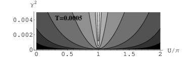
Figure 2: Iso-conductance plot in the $(U/W,\gamma^{2}/W)$ plane, at fixed T/W=0.0005. On each line, $G/G_{\tiny\mbox{IR}}=1-10^{-x}$ with $x$ ranging from 1 (dark) to 7 (bright).

In conclusion, it should be clear that methods of field theory give one a complete control of the linear conductance problem from the IR point of view. Apart from their practical use (the $8^{th}$ order could be calculated and the series Pade resummed to obtain full crossover curves) we hope that our results will provide useful benchmarks in assessing other approaches to the problem.

The authors would like to thank B. Doyon and A. Komnik for numerous enlightening discussions, as well as N. Andrei and P. Mehta for their patient explanations.

References

• (1) See for example D. Goldhaber-Gordon et al., Nature 391 (1998) 156; D. Goldhaber et al., Phys. Rev. Lett. 81 (1998) 5225.
• (2) P. Fendley, A. Ludwig and H. Saleur, Phys. Rev. B 52 (1995) 8934.
• (3) V. Bazhanov, S. Lukyanov, A. Zamolodchikov, Nucl.Phys. B 549 (1999) 529.
• (4) R. Konik, A. Ludwig and H.Saleur, Phys. Rev. B 66 (2002) 125304.
• (5) P. Mehta and N. Andrei, Phys. Rev. Lett. 96 (2006) 216802.
• (6) B. Doyon, “A new method for quantum impurity problems: the interacting resonant level model”, to appear.
• (7) L. Borda, K. Vladar and A. Zawadowski, cond-mat/0612583.
• (8) A. Komnik and A.O. Gogolin, Phys. Rev. Lett. 90 (2003) 246403.
• (9) P. Wiegmann and A.M. Finkel’stein, Sov. Phys. JETP 48 (1978) 102 .
• (10) V. Filyov and P. Wiegmann, Phys. Lett. 76A (1980) 283.
• (11) V.V. Ponomarenko, Phys Rev. B 48 (1993) 5265.
• (12) C. Callan, I. Klebanov, A. Ludwig and J. Maldacena, Nucl. Phys. B 422 (1994) 417; A. Recknagel and V. Schomerus, Nucl. Phys. B 545 (1999) 233.
• (13) N. Andrei, Phys. Lett. 87A (1982) 299.
• (14) J. Lowenstein, Phys. Rev. B 29 (1984) 4120.
• (15) F. Lesage and H. Saleur, Nucl. Phys. B 546 (1999) 585.
• (16) F. Lesage and H. Saleur, Phys. Rev. Lett. 82 (1999) 4540.