Phase behaviour of attractive and repulsive ramp fluids: integral equation and computer simulation studies

Abstract

Using computer simulations and a thermodynamically self consistent integral equation we investigate the phase behaviour and thermodynamic anomalies of a fluid composed of spherical particles interacting via a two-scale ramp potential (a hard core plus a repulsive and an attractive ramp) and the corresponding purely repulsive model. Both simulation and integral equation results predict a liquid-liquid de-mixing when attractive forces are present, in addition to a gas-liquid transition. Furthermore, a fluid-solid transition emerges in the neighbourhood of the liquid-liquid transition region, leading to a phase diagram with a somewhat complicated topology. This solidification at moderate densities is also present in the repulsive ramp fluid, thus preventing fluid-fluid separation.

I Introduction

The existence of a liquid-liquid (LL) equilibrium and density, diffusivity and structural anomalies in single component fluids has attracted considerable interest in the last decade. The density and diffusion anomalies present in liquid water (i.e. the existence of a maximum in the density within the liquid phase, and an increase in diffusion upon compression, up to a certain point) have long since been known, and have been reproduced by several of the existing interaction modelsTanaka (1996); Yamada et al. (2002); Xu et al. (2005); Brovchenko et al. (2005); Vega and Abascal (2005). Experimental evidence for LL coexistence has been found for phosphorousKatayama et al. (2000), triphenyl phosphiteTanaka et al. (2004), and $n$-butanolKurita and Tanaka (2005), and it has been suggested that this LL equilibrium might be the source of the anomalies encountered in water. Computer simulations predict the existence of LL equilibria not only in waterTanaka (1996); Yamada et al. (2002); Brovchenko et al. (2005) but also in other loosely coordinated fluids, such as siliconSastry and Angell (2003), carbonGhiringhelli et al. (2004) and silicaSaika-Voivod et al. (2000). Whether these transitions physically exist or not is still open to debate, since in most cases they correspond to supercooled states which are rendered experimentally inaccessible by crystallisation. However, closely related first order transitions between low and high density amorphous phases have indeed been found for waterMishima (1993), silicaMukherjee et al. (2001) and germanium oxideSmith et al. (1995).

While the use of realistic models can provide reasonable explanations for the experimental behaviour of a physical system, a more thorough description of the mechanisms underlying both LL phase transitions and density, diffusivity and related anomalies can be acquired via the study of simplified models. In the case of LL equilibrium and polyamorphism in molecular fluidsCohen et al. (1996) the simple model of Roberts and DebenedettiRoberts and Debenedetti (1996) has successfully accounted for the behaviour of network forming fluidsRoberts et al. (1996). On the other hand, since the pioneering work of Hemmer and StellHemmer and Stell (1970); Stell and Hemmer (1972) it is known that a simple spherically symmetric potential in which the repulsive interaction has been softened (in this case by the addition of a repulsive ramp to the hard core) can lead to the existence of a second (LL) critical point, as long as a first (liquid-vapour, LV) critical point existed due to the presence of a long range attractive component in the interaction potential. As well as the ramp potential, other simple models with two distinct ranges of interaction, such as the hard-sphere square shoulder-square well potential studied by Skibinsky et al.Skibinsky et al. (2004), have also been shown to exhibit LL equilibria. Indeed the presence of two interaction ranges explains the competition between two locally preferred structures (LPS) – a LPS being defined as an arrangement of particles which, for a given state point, minimises some local Helmholtz energy Tarjus et al. (2003). This competition between two LPS helps to rationalise the existence of polyamorphism and LL equilibria in single component glassy systems and fluidsTarjus et al. (2003).

More recently, the original model proposed by Hemmer and Stell has regained attention, especially since JaglaJagla (1999) stressed the similarities between the behaviour of the Hemmer-Stell ramp potential and the anomalous properties of liquid water. This has been further explored by Xu et al.Xu et al. (2005, 2006) who analysed the relationship between the LL transition and changes in the dynamic behaviour of fluids interacting via a soft core ramp potential with attractive dispersive interactions added. Gibson and WildingGibson and Wilding (2006) have recently presented an exhaustive study of a series of ramp potentials exhibiting LL transitions and density anomalies, whose relative position and stability with respect to freezing might be tuned by judicious changes in the interaction parameter. Moreover, Caballero and PuertasCaballero and Puertas (2006) have also focused on the relation between the density anomaly and the LL transition for this model system by means of a Monte Carlo based perturbation approach. The aforementioned authors find that, in this case, the density anomaly is absent when the range of the attractive interaction is sufficiently small.

In this work we shall refer to this interaction potential as the ‘attractive two-scale ramp potential’ (A2SRP). Additionally, when one considers the system without any attractive contribution, i.e. a hard-sphere core plus a repulsive ramp, as the ‘two-scale ramp potential’ (2SRP). Although it has been found that the system exhibits density anomalies, it is a possibility that LL transition is preempted by crystallisationKumar et al. (2005). In this purely repulsive model, the relation between static and dynamic anomalies has been explored in detailKumar et al. (2005); Sharma et al. (2006); Errington et al. (2006) (similar results have been found for a dumbbell fluid with repulsive ramp site-site interactionsNetz et al. (2006)) and the connection between these anomalies and structural order has been investigated by Yan et al.Yan et al. (2005) with the aid of the Errington-Debenedetti order mapErrington and Debenedetti (2001); Errington et al. (2003). These authors found that there is a region of structural anomalies (in which both translational and orientational order decrease as density is increased) that encapsulates the diffusivity and density anomaly region. The intimate relationship between transport coefficients, and the excess entropy was made clear first by Rosenfeld Rosenfeld (1977, 1999), and again later, specifically for the atomic diffusion, by Dzugutov Dzugutov (1996). Needless to say, a corollary of this relation is that any anomalous diffusion will be accompanied by an anomalous excess entropy. Recently this link has been shown to hold for both liquid silica and for the 2SRP model by Sharma et al. Sharma et al. (2006), and for the discontinuous core-softened model by Errington et al.Errington et al. (2006).

The principal objective of this work is to extend our knowledge of the phase behaviour of systems interacting via either attractive or purely repulsive two scale ramp potentials (A2SRP and 2SRP). To that purpose exhaustive Monte Carlo calculations have been performed in order to determine the phase boundaries of the gas, liquid and solid phases for both model systems up to moderate densities –slightly beyond the high density branch of the LL equilibrium. Self-consistent integral equation calculations performed on the A2SRP model complement the Monte Carlo results and agree qualitatively as to the location of the LL equilibria and quantitatively for the LV equilibria. The location of Widom’s line (the locus of heat capacity maxima) is obtained for both models. The temperature of maximum density (TMD) curve is obtained for the repulsive 2SRP model and correlated with the location of Widom’s line. The rich variety of phases present in these simple models will be illustrated in the calculated phase diagrams.

The structure of the paper is as follows; the model and computational procedures used herein are introduced in Section II. In Section III the most significant results are presented and discussed. Finally, the main conclusions and future prospects can be found in Section IV.

II Model and computational methods

The first model system consists of hard spheres of diameter $\sigma$, with a repulsive soft core and an attractive region. The interaction potential reads

$$u(r)=\left\{\begin{array}[]{ll}\infty&\mbox{if}\;r<\sigma\\ W_{r}-(W_{r}-W_{a})\frac{r-\sigma}{d_{a}-\sigma}&\mbox{if}\;\sigma\leq r\leq d_{a}\\ W_{a}-W_{a}\frac{r-d_{a}}{d_{c}-d_{a}}&\mbox{if}\;d_{a}<r\leq d_{c}\\ 0&\mbox{if}\;r>d_{c}\end{array}\right.$$ (1)

where $W_{r}>0$ and $W_{a}<0$. The values used here for the parameterisation of the model are the same as those used in Ref. Xu et al., 2005. Thus, energy units are defined by $|W_{a}|$, with the reduced temperature $T^{*}=k_{B}T/|W_{a}|$ ($k_{B}$ being the Boltzmann constant) and we have set $W_{r}/|W_{a}|=3.5$. The units of length are reduced with respect to the hard core diameter, and so one has $d_{a}/\sigma=1.72$, $d_{c}/\sigma=3.0$ and the reduced density is $\rho^{*}=\rho\sigma^{3}$ as usual. This set of parameter values and Eq.(1) define the A2SRP model. For the purely repulsive system, we have chosen the corresponding repulsive potential that would result from a Weeks-Chandler-AndersonWeeks et al. (1971) decomposition of Eq.(1), namely

$$u_{r}(r)=\left\{\begin{array}[]{ll}\infty&\mbox{if}\;r<\sigma\\ W_{r}-W_{a}-(W_{r}-W_{a})\frac{r-\sigma}{d_{a}-\sigma}&\mbox{if}\;\sigma\leq r\leq d_{a}\\ 0&\mbox{if}\;r>d_{a}\end{array}\right.$$ (2)

In Figure 1 both the attractive and purely repulsive interactions are illustrated.

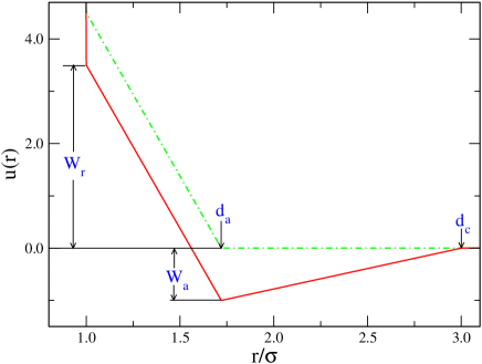
Figure 1: Attractive two scale ramp (A2SRP, solid line) and repulsive two scale ramp (2SRP, dash-dotted line) potential models.

II.1 The self consistent integral equation approach

The integral equation calculations are based on the Ornstein-Zernike relation, which for simple fluids readsOrnstein and Zernike (1914)

$$h(r_{12})=c(r_{12})+\rho\int c(r_{13})h(r_{32})d{\bf r}_{3}$$ (3)

where $h(r)$ is the total correlation function (related to the pair distribution function, $g$, by $h=g-1$) and $c(r)$ is the direct correlation function. This equation requires a supplementary relation, whose general form isMorita and Hiroik (23)

$$h(r)=\exp\left[-\beta u(r)+h(r)-c(r)+B(r)\right]-1$$ (4)

with $\beta=(k_{B}T)^{-1}$. In Eq.(4) the bridge function, $B(r)$, is a diagrammatic sum of convolutions of $h(r)$, and must be approximated. The simplest instance is the hyper-netted chain approximation (HNC), which implies $B(r)=0$. Interestingly, this approximation predicts the existence of a LL equilibrium in the square shoulder-square well model studied in Ref. Franzese et al., 2002 whereas for the A2SRP model only the LV equilibrium is reproduced. Moreover, in the case of the 2SRP model, it completely misses the density anomalyKumar et al. (2005). Preliminary calculations with a more elaborate closure such as the one proposed by Martynov, Sarkisov and Vompe (MSV)Martynov et al. (1999), show that although it turns out to be extremely accurate in the determination of the LV equilibria, it fails to capture the LL transition. However, one observes a second Widom line at moderate densities, which seems to indicate an anomaly in the region where the LL is expected to appear. This implies that thermodynamic consistency should play a central role if the LL transition or the density anomaly is to be found. This is confirmed by the results Kumar et al.Kumar et al. (2005) for the 2SRP model. A fairly successful self consistent approach is the so-called Hybrid Mean Spherical approximation (HMSA) which smoothly interpolates between the HNC and the Mean Spherical Approximation (MSA) closuresHansen and Zerah (1985); Zerah and Hansen (1986). The corresponding closure reads

$$g(r) = \exp(-\beta u_{r}(r))$$ (5)

$$\times\left(1+\frac{\exp[f(r)(h(r)-c(r)-\beta u_{a}(r))]-1}{f(r)}\right)$$

with the interpolating function $f(r)=1-\exp(-\alpha r)$. The repulsive component of the interaction given by Eq.(2), and the attractive component simply given by $u_{a}(r)=u(r)-u_{r}(r)$ with $u(r)$ having been defined in Eq.(1). Note that for the purely repulsive system, where $u_{a}=0$, one recovers the Rogers-Young (RY) closureRogers and Young (1984). The parameter $\alpha$ is fixed by requiring consistency between virial and fluctuation theorem compressibilities. With the virial pressure defined by

$$\beta P^{v}=\rho-\frac{2\pi}{3}\rho^{2}\int_{\sigma}^{d_{c}}r^{3}\frac{\partial u_{r}(r)}{\partial r}g(r)dr+\frac{2\pi}{3}\rho^{2}\sigma^{3}g(\sigma^{+})$$ (6)

and

$$\beta\kappa_{T}^{-1}/\rho=\left.\frac{\partial\beta P}{\partial\rho}\right|_{T}=1-4\pi\rho\int_{0}^{\infty}r^{2}c(r)dr.$$ (7)

Consistency could be implemented on a local level by equating

$$\beta\kappa_{T}^{-1}/\rho=\left.\frac{\partial\beta P^{v}}{\partial\rho}\right|_{T}.$$ (8)

Alternatively, one might use a global consistency. In this case, in the absence of spinodal lines, one can simply enforce the condition

$$\beta P^{v}(\rho,T)=\beta P^{\kappa}(\rho,T)$$ (9)

with

$$\beta P^{\kappa}(\rho,T)=\int_{0}^{\rho}\left[1-4\pi\rho\int_{0}^{\infty}r^{2}c(r;\rho^{\prime},T)dr\right]d\rho^{\prime}.$$ (10)

In the presence of spinodal lines one might use a mixed thermodynamic integration path, as suggested by Caccamo et al.Caccamo and Pellicane (2002). In this paper extensive use is made of the local consistency (LC) approach. We have also explored the use of global consistently (GC) as an alternative to overcome the deficiencies exhibited by the LC approach. From a practical point of view, in order to calculate the derivative of the virial pressure in Eq.(8), we shall assume that the parameter $\alpha$ is locally independent of the density, as is customary. For density independent potentials this leads to minor discrepancies when comparing the integrated pressures in Eq. (9), so both LC and GC approaches yield similar results Caccamo et al. (1993). Here the situation is somewhat different, as will be seen in the proceeding Section. Finally, the right hand side of Eq.(8) is explicitly calculated via

$$\left.\frac{\partial\beta P^{v}}{\partial\rho}\right|_{T} = \frac{2\beta P^{v}}{\rho}-1$$ (11)

$$-\frac{2\pi}{3}\rho^{2}\int_{\sigma}^{d_{c}}r^{3}\left(\frac{\partial u_{r}(r)}{\partial r}\right)\left(\frac{\partial g(r)}{\partial\rho}\right)dr$$

$$+\frac{2\pi}{3}\rho^{2}\sigma^{3}\left.\frac{\partial g(r)}{\partial\rho}\right|_{r=\sigma^{+}}$$

where the density derivative of the pair distribution function is obtained by iterative solution of the integral equation that results from differentiation of (3) and (5) with respect to density. This procedure, first proposed by BelloniBelloni (1988) is substantially more efficient than the classical finite differences approach when it comes to evaluating the derivative of $\beta P^{v}$. In addition to the density derivatives of the pair correlation function we have also evaluated the corresponding temperature derivatives in order to calculate the heat capacitySarkisov and Lomba (2005)

$$C_{v}^{*} = \frac{C_{v}}{Nk_{B}}-\frac{3}{2}$$ (12)

$$= 2\pi\rho\int\beta u(r)g(r)\left(\beta u(r)-\beta\left.\frac{\partial\omega(r)}{\partial\beta}\right|_{\rho}\right)r^{2}dr$$

where $\omega=h-c+B$. Note that the integral equations in terms of the derivatives of the correlation functions (either with respect to $\rho$ or $\beta$) are extremely well conditioned and are rapidly solved, even when starting from ideal gas initial estimates.

II.2 Simulation algorithms

Initially the principal aim was to establish whether the A2SRP model does indeed exhibit a fluid-fluid equilibrium. Therefore, in order to compute both the liquid-vapour and the LL equilibria, a procedure PRE_2005_71_046132 based on the algorithm of Wang and Landau PRL_2001_86_2050 ; PRE_2001_64_056101 was implemented. Subsequently, it was necessary to compute the equilibrium of the fluid phases with the low density solid phase. To that end use was made of thermodynamic integration frenkel_smit and the so-called Gibbs-Duhem integration techniquesfrenkel_smit ; mp_1993_78_1331 ; jcp_1993_98_4149 , which took advantage of the behaviour of the repulsive model in the low temperature limit. The use of two different methods in independent calculations provides a check on the quality of the results.

II.2.1 Wang-Landau-type algorithm

A more detailed explanation of the Wang-Landau procedure can be found elsewhere PRE_2005_71_046132 . Here, we shall restrict ourselves to outlining its most salient features. The algorithm fixes the volume and temperature and then samples over a range of densities ($N$) of the system. For each distinct density the Helmholtz energy function $F(N|V,T)$ is calculated. The procedure resembles, to some extent, well known grand canonical Monte Carlo methods frenkel_smit ; allen_tildesley , but using a different (previously estimated) weighting function for the different values of $N$. Once $F(N|V,T)$ is known for different values of $N$, one is able to compute the density distribution function for different values of the chemical potential, $\mu$, and extract the conditions for which the density fluctuations are maximal. This could indicate the presence of phase separation and eventually, by means of finite-size-scaling analysis, one can locate regions of two phase equilibrium and the locus of critical points.PRE_2005_71_046132 By following such a procedure one can easily compute the liquid-vapour (LV) equilibrium at high temperatures. The computation of the liquid-vapour equilibrium was predominantly performed with a simulation box of volume $V/\sigma^{3}=1000$ (i.e. box side length of $L^{*}\equiv L/\sigma=10$). In order to obtain a precise location of the critical point simulation runs were performed close to the estimated critical point for different system sizes: $L^{*}=6,7,8,9,10,11,$ and $12$. By means of re-weighting techniques and finite-size-scaling analysis, we have estimated the location of the critical point to be: $T^{*}_{c}=1.487\pm 0.003$, $\rho_{c}\sigma^{3}=0.103\pm 0.001$, and $p_{c}\sigma^{3}/|W_{a}|\equiv p_{c}^{*}\simeq 0.042$.

At low temperatures the LL equilibrium was found, but as the temperature was further reduced we were unable to obtain convergence in the estimates of the Helmholtz energy function, and the systems eventually formed a low density solid phase. Given this situation it was surmised that a triple point, if it exists, between the vapour and the two liquid phases, could not be stable, and the presence of a stable low density solid phase is most likely. After performing simulations at several temperatures, with different system sizes ($0\leq\rho\sigma^{3}\leq 0.55$, $L^{*}=6,8,10$), it was found that the LL equilibrium appeared for temperatures below $T^{*}\simeq 0.38$. Using the results for $L^{*}=10$, we can estimate the critical point for the LL equilibrium at $T_{c}^{*}\simeq 0.378\pm 0.003$, $\rho_{c}\sigma^{3}\simeq 0.380\pm 0.002$ and $(p^{*}_{c}/T^{*}_{c})\simeq 0.49\pm 0.01$.

II.2.2 Thermodynamic Integration: 2SRP model

In order to compute the phase equilibria between the low density solid and the fluid phases, it is useful to firstly consider the repulsive model. JaglaJagla (1999) computed the stability of different crystalline structures at $T=0$ for the repulsive model supplemented by a mean field attraction term, for a ramp model with $d_{a}/\sigma=1.75$, and found that the stable crystalline phases at low pressure correspond to the face-centred cubic (fcc) and hexagonal close packed (hcp) structures. On the other hand, in the limit $T\rightarrow 0$, and not too high a pressure the 2SRP model approaches an effective hard sphere system with diameter $d_{a}$. We can, then, expect the fcc structure to be the stable phase in the rangefrenkel_smit : $1.038(\sigma/d_{a})^{3}\leq\rho\sigma^{3}\leq\sqrt{2}(\sigma/d_{a})^{3}$, with the transition from the low density fluid to the solid at a pressure frenkel_smit of $\beta p\sigma^{3}\simeq 11.6\>(\sigma/d_{a})^{3}$. Assuming that the fcc is indeed the structure of the low density solid phase, and taking into account the low temperature limit for the 2SRP model one can use standard methods to study the equilibrium of this solid with the fluid phase(s).

In order to relate the two ramp models considered in this work, and to explain the procedures used to compute the phase diagram of the systems using thermodynamic and Gibbs-Duhem integration, it is useful to write down a generalised interaction potential, $u_{1}(r)$ using an additional ‘perturbation’ parameter, $\lambda$:

$$u_{1}(r|\lambda)=u_{r}(r)+\lambda u_{a}(r).$$ (13)

When $\lambda=0$, there are two interesting limits; when $T\rightarrow\infty$ the model approaches that of a system of hard spheres of diameter $\sigma$, whereas in the limit $T\rightarrow 0$ one once again encounters a hard sphere system, but now having a diameter of $d_{a}$. In order to compute the Helmholtz energy for condensed phases of the ramp potential systems, one can perform thermodynamic integration over the variable $\beta$ and the parameter $\lambda$. Thus one is able to compute the difference between the Helmholtz energy of a particular state, and the aforementioned hard sphere systems.

In the canonical ensemble the partition function can be written as:

$$Q_{1}=\frac{V^{N}}{\Lambda^{3N}N!}\int d{\bf R}^{*}\exp\left[-\beta U_{1}(V,{\bf R}^{*},\lambda)\right]$$ (14)

where $\Lambda$, the de Broglie thermal wavelength, depends on the temperature; ${\bf R}^{*}$ represents the reduced coordinates of the $N$ particles: ($\int d{\bf R}^{*}=1$), and $U_{1}$ is the potential energy (given by the sum of pair interactions $u_{1}(r|\lambda)$). The Helmholtz energy function is given by: $\beta F_{1}=-\log Q_{1}$. One can then write the Helmholtz energy per particle, $f=F/N$, as:

$$\beta f=\beta f^{id}+\beta f^{ex};$$ (15)

where the ideal contribution $f^{id}$ can be written as

$$\beta f^{id}=3\log\frac{\Lambda(T)}{\sigma}+\log(\rho\sigma^{3})-1.$$ (16)

and the excess part as

$$\beta f^{ex}=-\frac{1}{N}\log\left\{\int d{\bf R}^{*}\exp\left[-\beta U_{1}(V,{\bf R}^{*},\lambda)\right]\right\}.$$ (17)

In what follows we shall consider the Helmholtz energy as a function of the variables $N,V,T$, and $\lambda$ (or, equivalently, as $N,\rho,\beta$ and $\lambda$). We can then compute the derivatives of $\beta f^{ex}$ with respect to $\beta$ and $\lambda$. I.e.

$$\frac{\partial(\beta f^{ex})}{\partial\beta}=\frac{1}{N}\langle U\rangle$$ (18)

and

$$\frac{\partial(\beta f^{ex})}{\partial\lambda}=\frac{1}{N}\beta\langle U_{a}\rangle,$$ (19)

where the averaged quantity, $\langle U_{a}\rangle$, is given by:

$$\langle U_{a}\rangle=\left\langle\sum_{i=1}^{N-1}\sum_{j=i+1}^{N}u_{a}(r_{ij})\right\rangle.$$ (20)

On the other hand, using the well known thermodynamic relation:

$$\left(\frac{\partial F}{\partial V}\right)_{NT\lambda}=-p$$ (21)

one obtains

$$\frac{\partial(\beta f)}{\partial\rho}=\frac{\beta p}{\rho^{2}}.$$ (22)

For the 2SRP model $(\lambda=0)$, one can compute the Helmholtz energy of the low density solid using thermodynamic integration. As mentioned earlier, in the limit $T\rightarrow 0$ one has an effective hard sphere system of diameter $d_{a}$. The phase diagram of the hard sphere system frenkel_smit , the equation of state for the fluid jpcm_1997_9_8951 ; jcp_1969_51_635 and the equation of state for the solid jcp_1998_10_4387 are all well known. Thus

$$\beta f^{ex}(\rho,T)=\beta f_{hs}^{ex}(\rho d_{a}^{3})-\int_{0}^{T}\frac{U(T_{1})}{Nk_{B}T_{1}^{2}}\>dT_{1}.$$ (23)

where $\beta f_{hs}^{ex}(\rho d^{3})$ is the excess Helmholtz energy per particle in the fcc-solid phase and $U/N$ is the excess internal energy per particle. The integrand in (23) is well behaved in the limit $T\rightarrow 0$. Simulations have been undertaken for $N=500$, $\rho\sigma^{3}=0.24$ ($\rho d_{a}^{3}\simeq 1.2212$), for various temperatures; $T^{*}=0.025,~{}0.050,~{}0.10,~{}0.15,~{}0.20,\dots,0.45,~{}0.500$. At $T^{*}=0.500$ the system melts. The results for $U/T^{2}$ as a function of $T$ have been fitted using a polynomial. Thus we are able to obtain a function to compute the Helmholtz energy of the low density solid phase in the range $0<T^{*}<0.45$ at the reference reduced density of $\rho_{0}^{(s)}\sigma^{3}=0.24$.

In order to acquire data for the calculation of the fluid-low density solid equilibrium a number of simulations were performed for the low density solid phase, along several isotherms, having densities around $\rho_{0}^{(s)}$. The low density solid is stable only within a small region of the $\rho-T$ phase diagram, as can be seen in Fig. 10. The pressures in this stability range can be fitted to a polynomial,

$$\beta p_{s}(T,\rho)=\sum_{i=0}a_{i}^{(s)}(T)\rho^{i}.$$ (24)

We can then compute the Helmholtz energy of the low density solid, as a function of the density on each isotherm, using

$$\beta f(\rho_{1},T)=\beta f(\rho_{0},T)+\int_{\rho_{0}}^{\rho_{1}}\frac{\beta p(\rho,T)}{\rho^{2}}d\rho,$$ (25)

where $\rho_{0}=\rho_{0}^{(s)}$, and $\beta p(T,\rho)=\beta p_{s}(T,\rho)$.

The Helmholtz energy of the low-density fluid phase is computed using the results of several simulations, having $N=500$, at several temperatures and densities; typically $\rho\sigma^{3}=i\times 0.025$, with $i=1,2\dots,10$. In order to guarantee that the samples were indeed within the fluid phase the simulation runs were initiated from equilibrated configurations of temperature $T^{*}\simeq 2$. The pressure was fitted to a virial equation of state:

$$\frac{\beta p_{g}(\rho,T)-\rho}{\rho^{2}}=B_{2}(T)+B_{3}(T)\rho+B_{4}(T)\rho^{2}+\cdots,$$ (26)

which is then used in the calculation of the excess Helmholtz energy of the gas:

$$\beta f^{ex}(\rho,T)=\int_{0}^{\rho}\frac{\beta p_{g}(\rho_{1},T)-\rho_{1}}{\rho_{1}^{2}}\>d\rho_{1}$$ (27)

Using (15,16,26-27) one can compute the Helmholtz energy of the gas phase as a function of the density. The Helmholtz energies of the high density fluid can be computed using thermodynamic integration from the high temperature limit. Performing a number of simulations, with $N=500$, for different values of $\beta$ at a fixed reference density, $\rho_{l}$, we have

$$\beta f^{ex}(\rho_{l},\beta)=\beta f_{hs}^{ex}(\rho_{l}\sigma^{3})+\int_{0}^{\beta}\frac{U(N,\beta_{1},\rho_{l})}{N}\>d\beta_{1}$$ (28)

For selected temperatures several simulation runs are performed for various densities, and the results then are used to fit the equation of state of the liquid branch,

$$\beta p(T,\rho)=\sum_{i=0}a_{i}^{(l)}(T)\rho^{i}.$$ (29)

Similarly, we can compute the Helmholtz energy of the high density fluid at a given temperature by again performing simulations at several densities, and then fitting the results of the pressure as a function of the density and using (25) with $\rho_{0}=\rho_{0}^{(l)}$ where $\rho_{0}^{(l)}\sigma^{3}=0.40$. Once we have the equations of state for the low density fluid, the low density solid, and the high density fluid, and the corresponding Helmholtz energies at a certain reference density for each case, it is straightforward to compute the equilibria by locating the conditions at which both the chemical potential and pressure of two phases are equal.

II.2.3 Thermodynamic Integration: A2SRP Model

The Helmholtz energy of the fluid phases can be computed following the same procedures outlined in the previous subsection. In order to compute the Helmholtz energy of the low density solid phase one can perform thermodynamic integration starting from the repulsive model and integrating (19) at constant $\beta$, $\rho$, and $N$:

$$\beta f_{a}(\rho,T)=\beta f_{r}(\rho,T)+\frac{\beta}{N}\int_{0}^{1}\langle U_{a}(N,\rho,T,\lambda)\rangle\>d\lambda,$$ (30)

where the indices $a$ and $r$ indicate the A2SRP and the 2SRP models respectively. Such an integration was carried out using $\lambda=k\times 0.10$ (with $k=0,1,2,\cdots,10$) with $N=500$ at $\rho\sigma^{3}=0.24$ at the temperatures $T^{*}=0.30$ and $T^{*}=0.35$. The integrand $\langle U_{a}\rangle$ is well behaved in both cases. The Helmholtz energy of the A2SRP model low density solid phase at the reference density $\rho_{0}^{(s)}\sigma^{3}=0.24$ as a function of $T$ was parametrised via simulation results. Integration of (30) at two distinct temperatures provided a check of the numerical consistency. As for the 2SRP model various simulations were performed in the region of $\rho^{(s)}$ in order to compute the equation of state and the Helmholtz energy of the low density solid.

Thermodynamic integration was used to study the equilibrium between the low density solid and the high density liquid. The procedure was analogous to that used to study the low density solid-high density fluid equilibrium of the 2SRP model . To check the results of the LL equilibrium thermodynamic integration was performed at $T^{*}=0.35$. In order to do this the Helmholtz energy was calculated at the ‘reference’ reduced densities of 0.30 and 0.45 using the procedure derived from (28), and then by performing a simulation at $T^{*}=0.35$ at several densities. The results for the equation of state were fitted for both branches, and the conditions of thermodynamic equilibria were calculated. A good agreement (within the error bars) was found with the results from the Wang-Landau calculation.

II.2.4 Gibbs-Duhem Integration: 2SRP Model

The partition function, $Q(N,p,T,\lambda)$ in the isothermal-isobaric ($NpT$) ensemble can be written as frenkel_smit :

$$Q_{NpT}=\beta p\int dV\>\exp\left[-\beta pV\right]Q_{NVT}(N,V,T,\lambda).$$ (31)

The chemical potential, $\mu$ is given by

$$\beta\mu=-\frac{1}{N}\log Q_{NpT}.$$ (32)

Considering constant $N$, and $\mu=\mu(p,T,\lambda)$ one has:

$$d(\beta\mu)=\frac{E}{N}d\beta+\frac{V}{N}d(\beta p)+\frac{\beta U_{a}}{N}d\lambda.$$ (33)

where $E$ is the internal energy (including kinetic and potential contributions). Let us consider two phases, $\alpha$ and $\beta$, in conditions of thermodynamic equilibrium (i.e. equal values of $T$, $p$ and $\mu$); if one makes a differential change in some of the variables $\beta$, $(\beta p)$ and $\lambda$, thermodynamic equilibrium will be preserved if:

$$d[\Delta(\beta\mu)]=0=\Delta\bar{U}d\beta+\Delta\bar{V}d(\beta p)+\Delta\bar{U}_{a}d\lambda.$$ (34)

where $\Delta X$ expresses the difference between the values of the property $X$ in both phases, and ${\bar{X}}\equiv X/N$. In (34) we have considered equal values of the kinetic energy per particle in both phases (classical statistics).

In order to compute the fluid-low density solid equilibrium of the 2SRP model we make use of the Gibbs-Duhem integration scheme. As the starting point of the integration we consider the fluid-solid equilibrium of the effective hard sphere system, with diameter $d_{a}$ at $T=0$. We have integrated (34) for $\lambda=0$. After a number of short exploratory simulation runs, the Gibbs-Duhem integration computation for the 2SRP model was performed in three subsequent stages: i) low density fluid-low density solid equilibrium at low temperature, ii) fluid-low density solid at ‘higher’ temperatures, and iii) low density solid-high density fluid at low temperatures. For the first stage equation (34) was modified to obtain (in reduced units) the finite interval numerical approach:

$$\delta\left(\frac{p}{T}\right)\simeq\frac{\Delta\bar{U}}{T^{2}\Delta\bar{V}}\delta T.$$ (35)

The calculation of $\bar{U}$ and ${\bar{V}}$ for both phases at the estimated coexistence conditions was performed by Monte Carlo simulations with $N=500$, in the $NpT$ ensemble. At $T^{*}=0$ the coexistence of the fluid and the solid phases occurs frenkel_smit at $(p^{*}/T^{*})\simeq 2.286$ (i.e. $\simeq 11.6\times(\sigma/d_{a})^{3}$). A number of simulations ($T^{*}=0.01,0.02$ with $(p^{*}/T^{*})\simeq 2.29$) were used to estimate the initial values of the slope $d(p^{*}/T^{*})/dT^{*}$. The integration was then carried out from $T^{*}=0.01$ to $T^{*}=0.40$ with a step of $\delta T^{*}=0.01$,

In the second stage of the integration the coexistence temperature reaches a maximum, thus the independent variable in the integration was substituted for

$$\delta T\simeq\frac{T^{2}\Delta{\bar{V}}}{\Delta{\bar{U}}}\delta(p/T).$$ (36)

This integration was started from the pressure at which the temperature reaches $T^{*}=0.40$ (i.e. $(p^{*}/T^{*})\simeq 3.65$) using an integration step of $\delta(p^{*}/T^{*})=0.05$. Initially, the temperature increases with $p$ until the coexistence line reaches a maximum temperature; at this point the density of both phases is equal: ($T=0.422\pm 0.002$, $p^{*}/T^{*}=4.65\pm 0.05$, $\rho\sigma^{3}=0.260\pm 0.002$). For higher pressures the fluid density becomes higher than the low density solid density, and the temperature decreases with $p/T$. The third stage is initiated upon reaching $T^{*}=0.40$; which happens at $(p^{*}/T^{*})\simeq 6.33$. This involves reverting to the integration scheme given by (35), this time using $\delta T^{*}=-0.01$.

II.2.5 Gibbs-Duhem Integration: A2SRP Model

In order to compute the fluid-low density solid equilibria of the A2SRP system, this system is connected to the fluid-low density solid equilibria of the 2SRP model, by tuning the perturbation parameter $\lambda$ from $\lambda=0$ to $\lambda=1$, while maintaining the conditions of thermodynamic equilibrium, i.e. those of Eq. (34). For this system this connection stems from the initial state: $\lambda=0,T^{*}=0.34,(p^{*}/T^{*})=3.05$, which corresponds to the equilibrium between the low density solid with a lower density fluid. This was done by keeping $T$ constant and integrating numerically the equilibrium pressure as a function of $\lambda$, i.e.:

$$\delta(p^{*}/T^{*})\simeq-\frac{\Delta{\bar{U}}_{a}}{\Delta{\bar{V}}}\delta\lambda.$$ (37)

using $\delta\lambda=0.025$. The final point was found to be $(\lambda=1,p^{*}/T^{*}=-0.324)$, corresponding to a equilibrium between a low density solid with density $\rho^{*}=0.248$ and a low density liquid with $\rho^{*}=0.239$. Given the negative sign of the pressure the equilibrium found is metastable. From this point we can retake the Gibbs-Duhem integration (now for the attractive model, i.e. setting $\lambda=1$); using (36), with an integration step of $\delta(p^{*}/T^{*})=0.01$. As with the repulsive model a temperature maximum was found at $T_{M}^{*}\simeq 0.345$, $\rho\sigma^{3}\simeq 0.255$. However, in this case such a maximum seems to be metastable: $(p^{*}/T^{*})\simeq-0.01$. The solid-fluid equilibrium becomes thermodynamically stable at $p^{*}/T^{*}\approx 10^{-4}$ (where this coexistence line crosses the liquid-vapour equilibrium line). At higher pressures and lower temperatures this low density liquid-low density solid coexistence line will eventually coincide with the LL equilibrium line at a triple point. Beyond this a stable low density solid-high density liquid equilibrium will appear.

In order to obtain a precise estimate of the conditions for which the two liquid phases and the low density solid are in equilibria (i.e. the location of the triple point), Gibbs-Duhem integration was performed for the LL equilibrium. Both thermodynamic integration and the Wang-Landau procedure were used to calculate the LL equilibrium, at $T^{*}=0.35$. Both of the results agreed to within the error bars: ($\beta p\sigma^{3}\simeq 0.465$, with reduced densities of the liquid phase: $\rho_{1}\sigma^{3}\simeq 0.30$, and $\rho_{2}\sigma^{3}\simeq 0.46$). From this initial point the Gibbs-Duhem integrations of the phase equilibrium were carried out using (35) with $\delta T^{*}=0.0025$. The LL equilibrium line met the low density liquid-low density solid equilibrium at $T^{*}\simeq 0.331$, $(p^{*}/T^{*})\simeq 0.437$, with the three phases having reduced densities: $\rho_{\rm(low~{}density~{}solid)}\sigma^{3}\simeq 0.263$, $\rho_{\rm(low~{}density~{}liq.)}\sigma^{3}\simeq 0.293$ and $\rho_{\rm(high~{}density~{}liq.)}\sigma^{3}\simeq 0.48$ . Gibbs-Duhem integration was then used to calculate the low density solid-high density liquid equilibrium, starting from this triple point, using (35) with $\delta T^{*}=0.01$

II.2.6 Vapour-solid equilibrium

The computation of the density of the low density solid at equilibrium with the vapour phase for the A2SRP model is straightforward. In practice, due to the low pressure at which this equilibrium occurs, the $NpT$ simulations of the low density solid are undertaken at $\beta p\simeq 0$, again with $N=500$. This immediately yields an accurate estimate of the density of the solid in equilibrium with the vapour phase.

II.2.7 Details of the Gibbs-Duhem integration scheme

A simple predictor-corrector scheme was used to build up the coexistence lines. Generically one seeks the solution of:

$$\frac{dy}{dx}=f(x,y).$$ (38)

from some initial condition $x_{0},y_{0}$. In the present case the function $f(x,y)$ has to be computed via a pair of computer simulations. This result will be affected by statistical error. Using a set of discrete values $x_{i}=x_{0}+i\cdot h$, the following scheme was used:

$$y^{(p)}_{i+1}=y_{i}+\frac{1}{2}\left(3f_{i}-f_{i-1}\right)h$$ (39)

$$y_{i+1}=y_{i}+\frac{1}{2}\left(f_{i}+f_{i+1}\right).$$ (40)

with:

$$f_{i}=f(x_{i},y^{(p)}_{i})$$ (41)

where (39) and (40) are respectively the predictor and corrector steps. This simple algorithm is both accurate and robust.

III Results

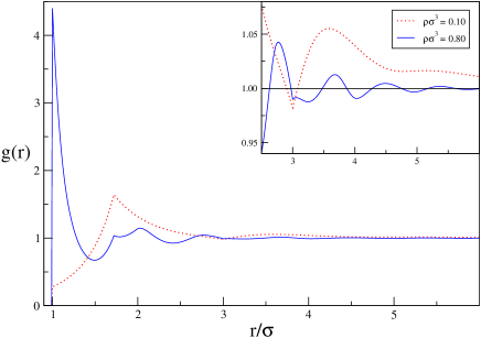
Figure 2: (Colour online) Pair distribution function for the A2SRP fluid at low ($\rho\sigma^{3}=0.10$) and high ($\rho\sigma^{3}=0.80$) densities at $T^{*}=1.8$. Inset: magnified view of the region $r/\sigma$ from 2.5 to 6.

In order to illustrate the two competing LPS that the A2SRP model system exhibits at low and high densities (or low and high pressures respectively) in Figure 2 we have presented the pair distribution functions for two representative states of the A2SRP model, obtained from the HMSA integral equation. The high density state is close to a hard sphere fluid of diameter $\sigma$, whereas the low density $g(r)$ corresponds to a fluid of soft particles of diameter $d_{a}=1.72\sigma$. The purely repulsive system leads to similar results, with only minor differences, due to the lack of dispersive forces (the sharp minima at $3\sigma$ are absent). It is clear that the LL transition will result from the ‘chemical equilibrium’ between two essentially different ‘fluids’ that stem from the same interaction.

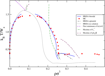
Figure 3: (Colour online) Phase diagram of the A2SRP model as obtained from the HMSA and Wang-Landau Monte Carlo simulations. HMSA results for the loci of maxima of $C_{v}^{*}$ (the Widom line), isothermal compressibility ($\rho\kappa_{T}/\beta$) and the set of thermodynamic states for which the first non trivial minimum of $h(r)$ vanishes. Additionally, the boundaries of the non-solution region of the integral equation and the thermodynamic spinodal of the LL transition are also depicted.

III.1 Liquid-vapour and liquid-liquid equilibria

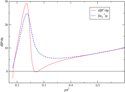
Figure 4: (Colour online) Inverse virial and fluctuation theorem compressibilities (solid and dashed curves respectively) as calculated using the HMSA integral equation at $T^{*}=0.38$ for the attractive model. Note how the consistency degrades when approaching the LL transition region (see Fig.3) to the point that the virial compressibility crosses a thermodynamic LL spinodal before hitting the LV spinodal, whereas the fluctuation theorem compressibility only detects the presence of the LV spinodal.

In order to calculate the phase diagram using the HMSA integral equation, one has to resort to thermodynamic integration. Although direct closed formulae for the chemical potential are available in the work of BelloniBelloni (1988), it has been the authors experience that better results are obtained when using thermodynamic integration. For a given state point, at density $\rho$ (on the right hand side of the phase diagram) and a subcritical inverse temperature $\beta$, one can obtain the free energy per particle along a mixed path of the form

$$f(\rho,\beta) =\frac{1}{\beta_{0}}\int_{0}^{\rho}(\beta p(\rho^{\prime},\beta_{0})-\rho)/\rho^{\prime 2}d\rho^{\prime}$$ (42)

$$+\frac{1}{\beta}\int_{\beta_{0}}^{\beta}U(\rho,\beta^{\prime})/Nd\beta^{\prime}+\log\rho\Lambda^{3}-1$$

where $\beta_{0}$ is a supercritical inverse temperatureWith this expression one is able to evaluate the chemical potential by using the relation

$$\beta\mu=\beta f+\frac{\beta p}{\rho}.$$

The phase equilibria can be determined by equating pressures and chemical potentials for both the gas and liquid phases, and for both the low density liquid and high density liquid phases.

The phase diagram thus obtained is plotted in Figure 3 together with the corresponding Monte Carlo estimates. Additionally, the curves corresponding to the loci of maxima of $C_{v}^{*}$ (the Widom line), maxima of the isothermal compressibility ($\rho\kappa_{T}/\beta$) and the set of thermodynamic states for which the first non trivial minimum of $h(r)$ vanishes are presented. This latter quantity separates supercritical states with gas-like local order from those with liquid-like orderSarkisov (2003). Interestingly, as found in the Lennard-Jones system with a completely different closureSarkisov (2003), these three singular lines are seen to converge towards the LV critical point. Although this should be expected from the locus of heat capacity and compressibility maxima, there is no apparent fundamental reason why this should also happen for the line of states for which the first minimum of $h(r)=0$. Moreover, we have found that similar results (with different locations for the critical point) are obtained using different closures, such as the HNC, Reference HNC or the MSV. Finally, one sees that the upper part of the binodal line is broken, since convergent solutions cease to exist before the critical point is reached. In fact, a small portion of the high temperature LV binodal has been obtained by extrapolation of the chemical potentials and pressures at lower vapour densities (for this reason the no-solution and the binodal curves cross). This is a well known limitation of a number of integral equation approaches, encountered even when treating the simple Lennard-Jones fluidLomba (1989).

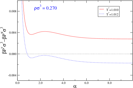
Figure 5: (Colour online) Residual inconsistency between virial and fluctuation theorem pressure as a function of the mixing parameter $\alpha$ in the HMSA closure (Eq. 5) for the 2SRP model.

As for the LL transition, in Figure 3 the HMSA binodal results obtained from the thermodynamic integration, its corresponding thermodynamic spinodal curve and the Wang-Landau Monte Carlo binodal estimates are presented. A second Widom line that crosses the LL binodal in the neighbourhood of the HMSA critical point is also found. As well as this, a second line of isothermal compressibility maxima seems to indicate the presence of a LL transition, approaching the simulation LL critical point. Note, however, that in this case the no-solution line does not provide any clue as to the presence of a phase separation. In contrast to the HMSA behaviour in the vicinity of the LV critical point, now the curves of $C_{v}^{*}$ and $\rho\kappa_{T}/\beta$ maxima do not converge to a common estimate of the critical point. This reveals a substantial inconsistency between the virial and the fluctuation theorem thermodynamics. This is best illustrated in Figure 4 where the virial and fluctuation theorem compressibilities are plotted. Here it is observed that the local consistency criterion of Eq.(8) leads to a good agreement for densities $\rho\sigma^{3}>0.4$, but a considerable inconsistency shows up at lower densities, corresponding to the LL transition (see Fig.3). The assumption of a density independent $\alpha$ parameter in the HMSA closure (Eq. 5) lies at the root of this failure. Thus, whereas the virial pressure predicts a LL transition, no diverging correlations appear near the thermodynamic spinodal, and the equation has solutions throughout the two phase region. This is in marked contrast to the results for the LV transition. On the other hand, in Fig.4 the large values of $(\partial\beta P/\partial\rho)_{T}$ in the region $0.2<\rho\sigma^{3}<0.3$ show that the fluid is almost incompressible, which is somewhat surprising, especially at these relatively low densities. This indicates that a solid phase (or a glassy state) may well be about to appear. We have attempted to explore alternatives to this breakdown in the LC approach. After an unsuccessful attempt to incorporate a linear density dependence on the $\alpha$ parameter in the HMSA interpolating function, in conjunction with a two parameter optimisation, we focused on the GC alternative expressed in Eq.(9). This can be easily implemented using the strategy proposed by Caccamo et al.Caccamo and Pellicane (2002). To make matters simpler, the GC HMSA calculations were restricted to the purely repulsive 2SRP model. At relatively high temperatures ($T^{*}\approx 2$) the procedure worked well and lead to results slightly better that those of the LC HMSA. However, as the temperature is lowered, one finds that the optimisation loop diverges even for relatively low densities. The reason behind this divergence is illustrated in Fig.5. It was observed that for two neighbouring states, a slight decrease in temperature upwardly displaces the residual inconsistency curve. As a consequence of this, when looking for consistency, the minima are now found to be greater than zero, thus the numerical iterations will lead to either a divergence or result in an oscillating behaviour. This also explains why the alternative procedure based on the implementation of a density dependent $\alpha$ failed as well. A completely parallel situation is to be found for the attractive potential model. It is now clear that a more accurate treatment of this type of soft core models requires not only the implementation of GC conditions on the pressure, but also the use of more flexible closure relations.

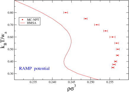
Figure 6: (Colour online) Zero pressure isobar calculated using the HMSA scheme and also by means of NPT MC simulation, for the A2SRP model.

Finally, a few words regarding the comparison of the integral equation estimates with the simulation results. As far as the LV transition is concerned, the HMSA predictions are satisfactory. The re-entrant behaviour that is clearly seen on the high density side of HMSA LV curve is also found in the MC estimates, and can be more clearly appreciated in the zero pressure isobar depicted in Fig. 6. Here we see that the errors in the density do not exceed 5 per cent. This partly reentrant behaviour is a characteristic indication of the proximity of a triple point, and has also been found in various water models Sanz et al. (2004); Brovchenko et al. (2005). On the other hand, whereas the LL critical temperature is reasonably well captured by the theory, the critical density is substantially underestimated, and the global shape of the LL equilibrium curve is not well reproduced. This can certainly be ascribed to the poor consistency of this HMSA approach in this region. Note, however, that this is the only integral equation theory, of those that we have checked, that captures the presence of the LL transition.

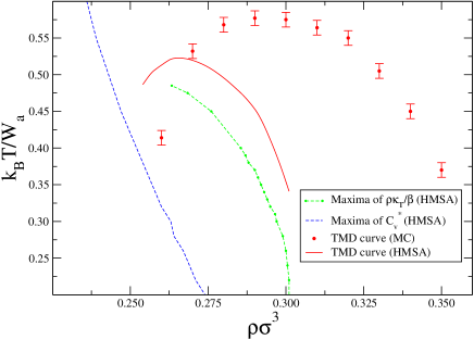
Figure 7: (Colour online) TMD curves as determined by HMSA calculations and NPT MC simulation for the purely repulsive model. Curves of maxima in the isothermal compressibility and heat capacity (Widom’s line) calculated using the HMSA closure.

When the attractive interactions are switched off, the LV transition disappears. The HMSA calculations yield lines of compressibility and heat capacity maxima that could be interpreted as indications of a possible LL transition (see Figure 7). These lines appear in approximately the same locations as in the attractive model (see Fig.3), which indicates that this feature is entirely due to the presence of the soft repulsive ramp in the interaction. The possibility of a LL transition in this model has already been speculated upon by Kumar et al.Kumar et al. (2005) on the basis of the low temperature asymptotic behaviour of a series of isochores. The same conclusion might well be drawn from this work; however, once again calculations at lower temperatures are hindered by lack of convergence. It shall be seen in the next section that the fluid-solid equilibrium preempts the LL phase separation.

As in Ref. Kumar et al., 2005, we are able to calculate the TMD curves (lines for which $(\partial T/\partial\rho)_{P}=0)$ from the minima of the pressure along isochoric curves (i.e. $(\partial P/\partial T)_{\rho}=0$). These results are plotted in Fig.7 and are compared with canonical MC estimates. The HMSA is qualitatively correct, with errors not exceeding 15 per cent. Nonetheless, once more the inconsistency of this LC HMSA is encountered in the results. From a simple thermodynamic analysis it is known that the line of maxima of the isothermal compressibility must cross the TMD curve at its maximum temperature Sastry et al. (1996). In Fig.7 one can observe that the curve of compressibility maxima disappears before reaching the TMD. Moreover, an extrapolation would locate the crossing at approximately $\rho\sigma^{3}=0.255$ and $T^{*}=0.496$, meanwhile the maximum of the TMD appears at $\rho\sigma^{3}=0.265$ and $T^{*}=0.523$. Whereas this can be accepted as being qualitatively correct, we find once more that global consistency must be enforced if quantitative predictions are to be obtained.

III.2 Solid-fluid equilibria

As explained in Subsection II.2, the complete phase diagram, including the fcc solid phase which appears at moderate densityJagla (1999), is computed by means of a combination of Wang-Landau Monte Carlo simulation (for the determination of LV and LL equilibrium curves), NPT MC zero pressure calculations to determine the VS equilibrium curves, standard thermodynamic integration and Gibbs-Duhem integration to evaluate the various fluid-solid equilibria. A detailed phase diagram is presented in Figs. 8 and 9. Note that for densities above $\rho\sigma^{3}=0.5$ other solid phases are possible. From Jagla’s workJagla (1999) (in which the relative stability of the zero temperature solid phases is explored) one can infer that at somewhat higher densities rhombohedric, cubic and hexagonal (hcp) phases could be expected. At still higher densities, for which the hard cores play the leading role, again the fcc and hcp phases will be the most stable structures. In any case, from Figure 8 one can already see a fairly complex phase diagram resulting from the coexistence of a vapour phase, two liquid phases and the fcc solid. Inset within Figure 8 we have enlarged the area of multiple coexistence, where one observes the presence of three triple points, namely two neighbouring triple points (lower inset) in which one liquid phase (denoted by L1), the vapour and the solid coexist, and a third triple point at lower temperature in which the two liquid phases (L1 and L2) coexist with the fcc solid. This latter triple point is also depicted in Fig.9 in a detail of the $P-T$ phase diagram.

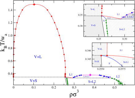
Figure 8: (Colour online) T-$\rho$ phase diagram of the attractive A2SRP model as obtained from computer simulation (circles, LV Wang-Landau MC estimates), (triangles, LL Wang-Landau MC estimates), (diamonds, MC NVT thermodynamic integration), (curves, Gibbs-Duhem integration) (VS equilibrium line, zero pressure NPT MC). The line connecting the liquid-vapour equilibrium points is drawn as a guide for the eye.

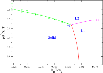
Figure 9: (Colour online) P-T phase diagram of the attractive A2SRP model as obtained from computer simulation. Points: thermodynamic integration, lines: Gibbs-Duhem integration. Legend as in Fig.8.

When the attractive interactions are switched off, even if we have seen that features such as the curves of compressibility and heat capacity maxima are hardly affected, the phase diagram simplifies substantially. Obviously, the LV transition disappears, and one is left with a rather peculiar fluid-solid transition (see Fig. 10). First, one observes that when density is increased along an isotherm starting from the low density fluid, the systems crystallises into an fcc phase, which melts upon further compression. At higher density values one could find the rhombohedric, cubic and hexagonal phases predicted by JaglaJagla (1999). This melting upon compression is similar to the behaviour of water. In the 2SRP model this is a purely energy driven transition: for certain densities the interparticle distance is necessarily $r<d_{a}$ and the repulsive spheres overlap, thus an ordered configuration no longer corresponds to an energy minimum. At sufficiently large densities ($\rho\sigma^{3}>0.9$), the hard cores will regain their controlling role and an entropy driven crystallisation will take place (into either fcc or hcp structures). In the intermediate region ($\rho\sigma^{3}>0.35$) the interplay between entropy and energy will give rise to a much more complex scenario with different solid phases in equilibrium with the fluid phase.

Finally, from the location of the fluid-solid equilibrium curve, it is now clear that a possible LL transition would be preempted by crystallisation. When comparing Figures 8 and 10 one can see that the effect of the dispersive interactions is to increase the stability of the liquid (fluid) phase with respect to the solid. Otherwise, the LL critical temperature happens to be fairly close to the the maximum temperature at which the fluid-solid equilibrium takes place ($T_{LL}^{*}=0.38$ vs $T_{FS}^{*}=0.42$).

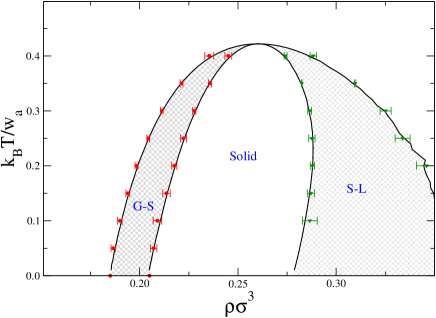
Figure 10: (Colour online) $\rho$-T phase diagram of the purely repulsive 2SRP model as obtained from computer simulation. Points: thermodynamic integration, lines: Gibbs-Duhem integration. Legend as in Fig.8.

IV Conclusions

In summary, we have presented a detailed study of both the attractive and the purely repulsive two scale ramp potential models, using both a self consistent integral equation (HMSA) and different Monte Carlo techniques. From this study, it becomes clear that the use of a thermodynamically consistent closure is essential if one wishes to capture the presence of the LL transition in the attractive model and the density anomaly of the repulsive fluid. Moreover, this type of model clearly highlights the shortcomings of local consistency criteria, such as those usually implemented in the HMSA. Unfortunately, our calculations using a global consistency condition on the pressure calculated from the virial and the isothermal compressibility only converge at high temperatures, well away from the LL and density anomaly region. This implies, that the closure is missing some essential features of the physical behaviour in the region controlled by the soft repulsive interactions. In order to bypass this limitation one should explore the use of other functional formsFernaud et al. (2000) or use an integro-differential approach of the Self Consistent Ornstein Zernike Approximation (SCOZA) Høye and Stell (1977, 1984) which has been recently implemented for systems with bounded potentialsMladek et al. (2006). Despite these limitations, the theoretical approach yields quantitatively correct estimates of the LV transition, the density anomaly and predicts the existence of a LL transition (although with a substantial underestimation of the LL critical density).

By means of extensive Monte Carlo simulations, we have unveiled the rather complicated shape of a significant part of the fluid-solid diagram for the A2SRP models, in which three triple points have been detected. In the purely repulsive model, one finds that the crystallisation preempts the liquid-liquid phase separation. This system has, in common with water, a solid phase that melts upon compression. In the intermediate region of the phase diagram, in which the hard core the the repulsive ramp are competing (i.e. when neither entropy nor energy but a subtle combination of both magnitudes leads the system behaviour) one should expect even more complex phase diagrams for both attractive and repulsive models. This will be the subject of future work.