Macroscopic Many-Qubit Interactions in Superconducting Flux Qubits

Abstract

Superconducting flux qubits are considered to investigate macroscopic many-qubit interactions. Many-qubit states based on current states can be manipulated through the current-phase relation in each superconducting loop. For flux qubit systems comprised of $N$ qubit loops, a general expression of low energy Hamiltonian is presented in terms of low energy levels of qubits and macroscopic quantum tunnelings between the many-qubit states. Many-qubit interactions classified by Ising type- or tunnel-exchange interactions can be observable experimentally. Flux qubit systems can provide various artificial-spin systems to study many-body systems that cannot be found naturally.

Introduction.$-$ The last decade has seen rapidly developing advanced material technologies that make it possible to investigate previously inaccessible quantum systems for quantum information and computation in solid-state systems. Especially, coherent manipulation of quantum states in tunable superconducting devices has enabled to demonstrate macroscopic qubits ChargeQ ; Mooij99 ; Yu and entangled states of qubits Pashkin ; Izmalkov ; Berkley . Experimentally, it has been shown that, in terms of pseudo-spins, different types of exchange interactions between two artificial-spins such as an Ising interaction for charge qubits Pashkin and flux qubits Izmalkov ; Majer and an XY interaction for phase qubits Berkley , can be realized and controlled by the system parameters.

It is believed that electrons are interacting in a pair. The interaction is called two-body interaction. Normally, in a number of spin systems such as spin chains and lattices, the two-body interactions in the spin pairs reveal rich many-electron physics. Understanding the many-electron effects is one of the most important researches in condensed matter physics. Additionally, in a strongly correlated electronic system, a low energy spin Hamiltonian can involve more than three spin interactions Thouless ; Roger ; MacDonald . Such multiple spin interactions are known to play a significant role for quantum phase transitions. However, multiple artificial-spin interactions are not yet investigated, although artificial-spin exchange (two-body) interactions are demonstrated in different types of solid-state qubit systems. This work aims to discuss, in a general framework, how artificial-multiple spin interactions are possible and realizable in superconducting qubit systems. In fact, flux qubit systems are shown to have an intrinsic property which is multiple artificial-spin interactions. Accordingly, flux qubit systems enable to study various artificial-spin systems corresponding to many-body systems unlikely found naturally.

In a superconductor, the macroscopic wavefunction can be written by $\psi({\bf r})=\sqrt{n^{*}}\,e^{i\varphi({\bf r})},$ where $n^{*}$ and $\varphi({\bf r})$ are the density and phase of Cooper pairs, respectively. $\psi({\bf r})$ describes the behavior of the entire ensemble of Cooper pairs in the superconductor. The supercurrent density in electromagnetic field is given by

$${\bf J}=\frac{q^{*}n^{*}}{m^{*}}\Big{(}\hbar\nabla\varphi({\bf r})-q^{*}{\bf A}({\bf r})\Big{)},$$ (1)

where $q^{*}$ and $m^{*}$ are respectively the charge and mass of Cooper pairs. Then, the current states of flux qubit loops are influenced by the variations of the phase $\varphi({\bf r})$ across Josephson junctions and the vector potential ${\bf A}({\bf r})$. A change of current state in a qubit loop results in a change of current states in other qubit loops because (i) the change of Josephson junction phases in superconducting loops coupling qubits mediates the change of the currents states of all qubits and (ii) the circulating current in the qubit produces the induced magnetic flux that influences on all other qubits. In experiments, several ways to make two- or four-flux qubits interacting have been employed. Disconnected supconducting loops, as the indirect way, are coupled inductively Izmalkov ; Majer by means of the induced magnetic flux. Other direct ways are to introduce connecting superconducting loops Kim ; Kim2006 ; Ploeg , which is called phase coupling. Consequently, many flux qubits defined by current states can interact all together, which can be observable in experiments.

We present a general expression of $N$-qubit Hamiltonian describing low energy physics. The Hamiltonian is determined by the low level energies and the tunneling amplitudes between $N$-qubit states in the flux qubit systems. We define two types of many-qubit exchange interactions originating from the energy differences of many-qubit states and the macroscopic quantum tunneling between the states. Further, it is shown that a specific coupling scheme enables to map flux qubit systems into many-body systems.

Model.$-$ We consider a general model including the inductive and phase coupling ways. The $N$ flux qubit systems are composed of $N$ qubit loops with $N^{\prime}$ loops connecting the qubit loops. Primed (unprimed) indices will indicate qubit (connecting) loops. The charging energy of Josephson junctions in the $N(N^{\prime})$ qubit (connecting) loops is given by

$${\cal H}_{C}=\!\frac{1}{2}\!\left(\frac{\Phi_{0}}{2\pi}\right)^{2}\!\!\bigg{(}\sum^{N}_{i=1}\!\sum_{\alpha}C^{\alpha}_{i}\dot{\varphi}^{2}_{i\alpha}\!+\!\sum^{N^{\prime}}_{i^{\prime}=1}\!\!\sum_{\alpha^{\prime}}C^{\alpha^{\prime}}_{i^{\prime}}\dot{\varphi}^{2}_{i^{\prime}\alpha^{\prime}}\bigg{)},$$ (2)

where $C(C^{\prime})$ are the capacitance of the Josephson junctions in the qubit (connecting) loops. $\Phi_{0}=h/2e$ is the unit flux quantum. $\alpha(\alpha^{\prime})$ rely on the number of Josephson junctions in the qubit (connecting) loops. The inductive energy is given by

$${\cal H}_{L} = \sum_{i,j=1}^{N}\frac{1}{2}\left(L^{(ij)}+\delta_{ij}L^{(i)}_{K}\right)I_{i}I_{j}+\sum_{i,i^{\prime}=1}^{N,N^{\prime}}{\cal L}^{(ii^{\prime})}I_{i}I^{\prime}_{i^{\prime}}$$ (3)

$$+\sum_{i^{\prime},j^{\prime}=1}^{N^{\prime}}\frac{1}{2}\left(L^{\prime(i^{\prime}j^{\prime})}+\delta_{i^{\prime}j^{\prime}}L^{\prime(i^{\prime})}_{K}\right)I^{\prime}_{i^{\prime}}I^{\prime}_{j^{\prime}},$$

where $I_{i}(I^{\prime}_{i^{\prime}})$ are the circulating currents in the qubit (connecting) loop $i(i^{\prime})$. $L^{(ii)}=L^{(i)}_{S}$ is the self-inductance for the qubit loop $i$. For $i\neq j$, $L^{(ij)}$ is the mutual inductance between the qubits $i$ and $j$. $L^{(i)}_{K}$ is the kinetic-inductance Kim ; Bloch ; MajerAPL in the qubit loop $i$. Similarly, $L^{\prime(i^{\prime})}_{S}$, $L^{\prime(i^{\prime})}_{K}$, and $L^{\prime(i^{\prime}j^{\prime})}$ are denoted for the connecting loops. ${\cal L}^{(ii^{\prime})}$ is the mutual inductance between the qubit loop $i$ and the connecting loop $i^{\prime}$. Finally, the Josephson energy of the junctions is given by

$${\cal H}_{J}\!=\!\sum^{N}_{i=1}\!\sum_{\alpha}2E^{\alpha}_{Ji}\sin^{2}\frac{\varphi^{\alpha}_{i}}{2}+\sum^{N^{\prime}}_{i^{\prime}=1}\sum_{\alpha^{\prime}}2E^{\prime\alpha^{\prime}}_{Ji^{\prime}}\sin^{2}\frac{\varphi^{\alpha^{\prime}}_{i^{\prime}}}{2},$$ (4)

where $E_{J}$’s are the Josephson energy of junctions in the qubit and connecting loops.

Fluxoid quantization.$-$ By integrating Eq. (1) along the closed path in the $i$-th loop, the fluxoid quantization gives the boundary conditions,

$$L^{(i)}_{K}I_{i}/\Phi_{0}=n_{i}-\frac{1}{2\pi}\sum_{\alpha}\varphi^{\alpha}_{i}-f_{i},$$ (5)

where $\varphi^{\alpha}_{i}$ is the phase across the Josephson junction $\alpha$, $n_{i}$ is an integer, and $f_{i}=f^{(i)}_{\mathrm{ext}}+f^{(i)}_{\mathrm{ind}}$ consists of an external and induced magnetic fields, i.e., $f^{(i)}_{\mathrm{ext}}=\Phi_{i}/\Phi_{0}$ and $f^{(i)}_{\mathrm{ind}}=\sum^{N}_{j=1}L^{(ij)}I_{j}/\Phi_{0}+\sum^{N^{\prime}}_{i^{\prime}=1}{\cal L}^{(ii^{\prime})}I^{\prime}_{i^{\prime}}/\Phi_{0}$. Similarly, the boundary conditions in the connecting loops can be given. From the boundary conditions, the total energy can be reexpressed as a function of the phases, $\{\varphi_{i}\}$ and their time derivatives, $\{\dot{\varphi}_{i}\}$.

$N$-qubit Hamiltonian.$-$ The number of Cooper pairs, $n$, and the phase of wavefunction, $\varphi$, are non-commuting variables, i.e., $[\varphi,n]=i$, such that the canonical momentum, $P_{\varphi}$, can be introduced as $P_{\varphi}=n\hbar=-i\hbar\partial_{\varphi}$ Mooij94 , where $n=q/2e$ with the charge from the Josephson relation, $q=C(\Phi_{0}/2\pi)\dot{\varphi}$. When the charging energy is much smaller than the Josephson energy, the phase is well-defined while the number is strongly fluctuating. The charging energy ${\cal H}_{C}(\{\dot{\varphi}_{i}\})$ plays a role of kinetic energy for a particle in an effective potential defined by $U(\{\varphi_{i}\})={\cal H}_{L}(\{\varphi_{i}\})+{\cal H}_{J}(\{\varphi_{i}\})$.

In the three-Josephson junction qubit loops ($\alpha\in\{a,b,c\}$) with $E^{b,c}_{Ji}=E_{Ji}$ and $\varphi^{b,c}_{i}=\varphi_{i}$, the effective potential has the $2^{N}$ local minima corresponding to the $2^{N}$ basis, $\{\left|m_{1},\cdots,m_{N}\right\rangle\}$ , of the $N$ qubits with $m_{i}=\uparrow$ and $\downarrow$ for $i=1,\cdots,N$. The values of $\{\varphi_{i}\}$ at the local minimum corresponding to the state $\left|m_{1},\cdots,m_{N}\right\rangle$ are denoted by $\{\varphi^{0}_{i;m_{1}\cdots m_{N}}\}$. Then, $\{\varphi^{0}_{i;m_{1}\cdots m_{N}}\}$ determines the current state of flux qubit $i$ by the current-phase relation.

In the low energy limit, one can employ a tight-binding approximation in which the $2^{N}$ states of $N$ qubits correspond to $2^{N}$-lattice sites. In the $2^{N}$ basis, $\{\left|m_{1},\cdots,m_{N}\right\rangle\}$, the low energy $N$ qubit-Hamiltonian matrix can be written as

$${\cal H}_{N}=\sum_{j_{1},\cdots,j_{N}\in\{0,x,y,z\}}C_{j_{1}\cdots j_{N}}\;\mbox{\boldmath$\sigma$}^{j_{1}}_{1}\otimes\cdots\otimes\mbox{\boldmath$\sigma$}^{j_{N}}_{N},$$ (6)

where $\mbox{\boldmath$\sigma$}^{0}(\mbox{\boldmath$\sigma$}^{x,y,z})$ are the identity (Pauli) matrices. The coefficients are obtained by

$$C_{j_{1}\cdots j_{N}}=\frac{1}{2^{N}}\mathrm{Tr}\left[\mbox{\boldmath$\sigma$}^{j_{1}}_{1}\otimes\cdots\otimes\mbox{\boldmath$\sigma$}^{j_{N}}_{N}\;{\cal H}_{N}\right].$$ (7)

The diagonal components of the Hamiltonian matrix are the level energies, $E_{m_{1},\cdots,m_{N}}$, at the local minima, $\{\varphi^{0}_{i;m_{1}\cdots m_{N}}\}$. The level energies are given by

$$E_{m_{1},\cdots,m_{N}}=\frac{\hbar}{2}\sum_{i=1}^{N}\omega_{i;m_{1},\cdots,m_{N}}+U(\{\varphi^{0}_{i;m_{1}\cdots m_{N}}\}),$$ (8)

where the characteristic oscillating frequencies are $\omega^{2}_{i;m_{1},\cdots,m_{N}}=\frac{1}{M_{i}}\frac{\partial^{2}}{\partial\varphi^{2}_{i}}U(\{\varphi_{i}\})|_{\{\varphi^{0}_{i;m_{1},\cdots,m_{N}}\}}$ with an effective mass $M_{i}=\left(\frac{\Phi_{0}}{2\pi}\right)^{2}C^{(i)}_{\rm eff}$ and effective capacitance $C^{(i)}_{\rm eff}$ in the harmonic oscillator approximation Orlando .

Generally, the macroscopic tunneling processes between any two many-qubit states are possible due to the quantum fluctuation originating from the kinetic energy. The off-diagonal components are the macroscopic quantum tunneling amplitudes, i.e.,

$$t\,\,:\,\left|m^{\prime}_{1},\cdots,m^{\prime}_{N}\right\rangle\Longleftrightarrow\left|m_{1},\cdots,m_{N}\right\rangle$$ (9)

for the tunneling between the two states, $\left|m^{\prime}_{1},\cdots,m^{\prime}_{N}\right\rangle$ and $\left|m_{1},\cdots,m_{N}\right\rangle$. The tunneling amplitudes can be calculated by the well-known numerical methods such as WKB approximation, instanton method, and Fourier grid Hamiltonian method Kim03 . The tunneling process, $\left|\uparrow\uparrow\uparrow\cdots\uparrow\right\rangle\Longleftrightarrow\left|\downarrow\uparrow\uparrow\cdots\uparrow\right\rangle$, describes the first pseudo-spin flip. Such a tunneling process that describes only one pseudo-spin flip among the $N$ qubits is called single qubit tunneling, $t_{1}$. If the $N$ qubits are flipped for tunneling, the tunneling processes can be called N-qubit tunneling, $t_{N}$, e.g., $\left|\downarrow\uparrow\uparrow\cdots\downarrow\right\rangle\Longleftrightarrow\left|\uparrow\downarrow\downarrow\cdots\uparrow\right\rangle$. Normally, single qubit tunneling amplitudes are much larger than other multiple qubit ones. However, when a multiple qubit tunneling amplitude is larger than single qubit one, the multiple qubit tunneling processes can play an important role in determining the property of eigenstates of the system Kim06 ; Kim07 .

Many-qubit interaction.$-$ Actually, Eq. (6) describes any $N$ qubit system including all types of many-qubit interactions. Let us expand the low energy $N$ qubit-Hamiltonian matrix in terms of qubit interactions;

$${\cal H}_{N}\!=\!H_{0}\!+\!\sum_{i}H^{(i)}_{1}+\sum_{i<j}H^{(ij)}_{2}+\!\!\sum_{i<j<k}H^{(ijk)}_{3}+\cdots+H^{(1\cdots N)}_{N},$$ (10)

where $H_{0}=(1/2^{N})\mathrm{Tr}\left[{\cal H}_{N}\right]$ and the qubits are described by $H^{(i)}_{1}=\varepsilon_{i}\ \mbox{\boldmath$\sigma$}^{z}_{i}+t^{(i)}_{1}\mbox{\boldmath$\sigma$}^{x}_{i}$ with the energy difference $2\varepsilon_{i}$ and the tunneling amplitude $t^{(i)}_{1}$ between the two states of the qubit $i$. Qubit interactions are denoted by two-qubit interactions $H^{(ij)}_{2}$, three-qubit interactions $H^{(ijk)}_{3}$, and so on. Then, the $N$-qubit interaction is presented by

$$H^{(1\cdots N)}_{N}=\sum_{j_{1},\cdots,j_{N}\in\{x,y,z\}}C_{j_{1}\cdots j_{N}}\;\mbox{\boldmath$\sigma$}^{j_{1}}_{1}\otimes\cdots\otimes\mbox{\boldmath$\sigma$}^{j_{N}}_{N}.$$ (11)

We define the $N$-qubit exchange coupling constant as

$$J^{(N)}_{z\cdots z}=C_{z\cdots z}=\frac{1}{2^{N}}\mathrm{Tr}\left[\mbox{\boldmath$\sigma$}^{z}_{1}\otimes\cdots\otimes\mbox{\boldmath$\sigma$}^{z}_{N}\;{\cal H}_{N}\right],$$ (12)

which has a form of Ising type exchange interaction for $N$ qubits. For other terms of the $N$-qubit interaction, the coefficients of the terms can be called $N$-qubit tunnel-exchange coupling constants, e.g.,

$$J^{(N)}_{x\cdots y\cdots z}=C_{x\cdots y\cdots z}=\frac{1}{2^{N}}\mathrm{Tr}\left[\mbox{\boldmath$\sigma$}^{x}_{1}\otimes\cdots\mbox{\boldmath$\sigma$}^{y}_{i}\cdots\otimes\mbox{\boldmath$\sigma$}^{z}_{N}\;{\cal H}_{N}\right],$$

since the off-diagonal components of the Hamiltonian matrix result from the hopping (tunneling) between the sites (states).

Two qubit systems.$-$ For two qubit systems, the two-qubit interaction is given by $H^{(12)}_{2}=\sum_{j\in\{x,y,z\}}J^{(2)}_{jj}\mbox{\boldmath$\sigma$}^{j}_{1}\otimes\mbox{\boldmath$\sigma$}^{j}_{2},$ where $J^{(2)}_{xx}=-(t^{a}_{2}+t^{b}_{2})/2$, $J^{(2)}_{yy}=(t^{a}_{2}-t^{b}_{2})/2$, and $J^{(2)}_{zz}=\left(E_{\uparrow\uparrow}-E_{\uparrow\downarrow}-E_{\downarrow\uparrow}+E_{\downarrow\downarrow}\right)/4$. The two-qubit tunneling amplitudes, (i) $t^{a}_{2}$ and (ii) $t^{b}_{2}$, describe the tunneling processes, (i) $\left|\uparrow\uparrow\right\rangle\Longleftrightarrow\left|\downarrow\downarrow\right\rangle$ in the parallel pseudo-spin states and (ii) $\left|\uparrow\downarrow\right\rangle\Longleftrightarrow\left|\downarrow\uparrow\right\rangle$ in the anti-parallel pseudo-spin states. As expected, the exchange coupling constant $J^{(2)}_{zz}$ is the energy difference between the parallel and anti-parallel pseudo-spin states. The two-qubit tunnelings contribute to the pseudo-spin exchange interaction. Then, $H^{(12)}_{2}$ has a form of XYZ model for two-pseudo spins. $t^{a}_{2}\ll t^{b}_{2}$ gives an XXZ pseudo-spin model and, for $J^{(2)}_{zz}=0$, i.e., $E_{\uparrow\uparrow}+E_{\downarrow\downarrow}=E_{\uparrow\downarrow}+E_{\downarrow\uparrow}$, an XY pseudo-spin model. For $t^{a,b}_{2}\ll J^{(2)}_{zz}$, $H^{(12)}_{2}$ becomes an Ising pseudo-spin model. This shows that various types of pseudo-spin models can be realized by manipulating the system parameters.

Three qubit systems.$-$ Next, for comparison, let us consider a two-qubit interaction of three qubit system given by $H^{(12)}_{2}=\sum_{j\in\{x,y,z\}}J^{(2)}_{jj0}\mbox{\boldmath$\sigma$}^{j}_{1}\otimes\mbox{\boldmath$\sigma$}^{j}_{2}+J^{(2)}_{xz0}\mbox{\boldmath$\sigma$}^{x}_{1}\otimes\mbox{\boldmath$\sigma$}^{z}_{2}+J^{(2)}_{zx0}\mbox{\boldmath$\sigma$}^{z}_{1}\otimes\mbox{\boldmath$\sigma$}^{x}_{2}$, where $J^{(2)}_{xx0}=-(\bar{t}^{a}_{2}+\bar{t}^{b}_{2})/4-(\underline{t}^{a}_{2}+\underline{t}^{b}_{2})/4$, $J^{(2)}_{yy0}=(\bar{t}^{a}_{2}-\bar{t}^{b}_{2})/4+(\underline{t}^{a}_{2}-\underline{t}^{b}_{2})/4$, and $J^{(2)}_{zz0}=(E_{\uparrow\uparrow\uparrow}-E_{\uparrow\downarrow\uparrow}-E_{\downarrow\uparrow\uparrow}+E_{\downarrow\downarrow\uparrow})/8+(E_{\uparrow\uparrow\downarrow}-E_{\uparrow\downarrow\downarrow}-E_{\downarrow\uparrow\downarrow}+E_{\downarrow\downarrow\downarrow})/8$. Here, $\bar{t}$($\underline{t}$) denote the two-qubit tunnelings for the up(down) state of the third pseudo-spin. Compared to the two-qubit interaction in two-qubit systems, interestingly, there are the two extra tunnel-exchange coupling terms, $J^{(2)}_{xz0}$ and $J^{(2)}_{zx0}$, mediated by the single-qubit tunnelings.

In the three-qubit interaction $H^{(123)}_{3}$, the three-qubit exchange coupling constant is given by $J^{(3)}_{zzz}=(E_{\uparrow\uparrow\uparrow}-E_{\uparrow\downarrow\uparrow}-E_{\downarrow\uparrow\uparrow}+E_{\downarrow\downarrow\uparrow})/8-(E_{\uparrow\uparrow\downarrow}-E_{\uparrow\downarrow\downarrow}-E_{\downarrow\uparrow\downarrow}+E_{\downarrow\downarrow\downarrow})/8$. Also, the single- and two-qubit tunnelings as well as the three-qubit tunnelings give rise to the three-qubit tunnel-exchange coupling constants. Especially, if the three-qubit tunnelings are stronger than the two-qubit tunnelings, the ground state can be in a Greenberger-Horne-Zeilinger (GHZ) and if the two-qubit tunnelings are stronger than the three-qubit tunnelings, a W-state can be generated in an excited state Kim07 .

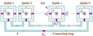
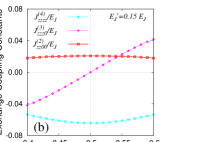
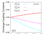
Figure 1: (Color online) Top: (a) A $N$ flux qubit system with one connecting loop. The $N$ superconducting loops are connected by a connecting loop interrupted by a Josephson junction, $E^{\prime}_{J}$. In each qubit loop, the diamagnetic (paramagnetic) current states assigned by $\left|\downarrow\right\rangle(\left|\uparrow\right\rangle)$, are superposed, which makes the loop being regarded as a qubit. $\odot$ (oppositely $\otimes$) denote the directions of the applied and induced magnetic fields, $f_{i}=\Phi_{i}/\Phi_{0}$, in the qubit loop $i$. $I_{i}(I^{\prime})$ stand for the currents in the qubit $i$ (connecting) loop. $E_{J}$’s are the Josephson coupling energies of the Josephson junctions in the connecting and qubit loops. The fluxoid quantization in the connecting loop gives rise to the boundary condition connecting the phases, $\varphi_{i}$, across each Josephson junction. Both the mutual inductances and the fluxoid quantization make it possible to realize many-qubit interactions in the $N$ flux qubit system. The many-qubit interactions are defined in the text. Bottom: Multiple qubit exchange coupling constants, $J^{(4)}_{zzzz}$, $J^{(3)}_{zzz0}$, and $J^{(2)}_{zz00}$, in the four qubits ($N=4$) as a function of (b) the applied magnetic field $f=f^{(i)}_{\rm ext}$ ($i=1,\cdots,4$) for $E^{\prime}_{J}=0.15E_{J}$ and (c) the Josephson energy $E^{\prime}_{J}$ for $f=0.45$. Other parameters are $n_{i}=n^{\prime}=0$ and $E^{\alpha}_{J}=E_{J}(\alpha\in\{a,b,c\})$.

Multiple qubit systems.$-$ To explore many-qubit interactions explicitly, let us consider a specific multiple-qubit system in Fig. 1 (a). For simplicity, the inductances are assumed to be very small and then the inductive energy can be negligible. The boundary conditions for (i) the qubit loops and (ii) the connecting loop are reduced to (i) $2\varphi_{i}+\varphi^{a}_{i}=2\pi(n_{i}-f^{(i)}_{\rm ext})$ and (ii) $\varphi^{\prime}=2\pi n^{\prime}-\sum^{N}_{i=1}\varphi^{a}_{i}$. The effective potential is given as $U\!\!\!=\!\!\!\sum^{N}_{i=1}\left[4E_{J}\sin^{2}\frac{\varphi_{i}}{2}+2E^{a}_{J}\sin^{2}\pi(n_{i}-f^{(i)}_{\rm ext}-\varphi_{i}/\pi)\right]+2E^{\prime}_{J}\sin^{2}\pi\left[n^{\prime}-\sum^{N}_{i=1}(n_{i}-f^{(i)}_{\rm ext}-\varphi_{i}/\pi)\right].$

For the four qubit system $(N=4)$, we plot the exchange coupling constants as a function of $f=f^{(i)}_{\rm ext}$ and $E^{\prime}_{J}$ in Fig. 1 (b) and (c), respectively. At the co-resonance point, $f=0.5$, the three-qubit interaction disappears while the two- and four-qubit interaction strengths reach their maximum values in Fig. 1 (b). The sign of the three-qubit interaction is changed from negative for $f<0.5$ to positive for $f>0.5$. As $E^{\prime}_{J}$ increases, the two-, three-, and four-qubit interactions increase monotonically in Fig. 1 (c).

Interestingly, the four-qubit interaction is stronger than the two- and three-qubit interactions. That is, $J^{(4)}_{zzzz}\approx 3J^{(2)}_{zz00}$. Also, the three-qubit interaction can be stronger than the two-qubit interaction for a certain applied magnetic field. This result seems to be counterintuitive. However, for an $N$ qubit system, the result can be understood from Eq. (5) and the boundary condition of the connecting loop, without the assumption, $L^{\prime}_{K}I^{\prime}/\Phi_{0}=n^{\prime}-(1/2\pi)(\varphi^{\prime}+\sum^{N}_{i=1}\varphi^{a}_{i})-f^{\prime}_{\mathrm{ind}},$ where $f^{\prime}_{\mathrm{ind}}=L^{\prime}I^{\prime}/\Phi_{0}+\sum^{N}_{i=1}{\cal L}^{(i)}_{M}I_{i}/\Phi_{0}$ with the mutual inductance ${\cal L}^{(i)}_{M}$. When one superconducting loop couples all qubit loops, all qubits are interconnected through the effective flux $f_{\rm eff}\equiv(1/2\pi)\sum^{N}_{i=1}\varphi^{a}_{i}$ as well as $f^{\prime}_{\mathrm{ind}}$. Normally, the induced flux is much smaller than the effective flux, i.e., $f^{(i)}_{\mathrm{ind}},f^{\prime}_{\mathrm{ind}}\ll f_{\rm eff}$, so that much stronger many-qubit interaction for the effective flux than for the induced magnetic flux can be expected. Therefore, if the $N$-qubit interaction is much stronger than other quit interactions, ${\cal H}_{N}\approx H^{(1\cdots N)}_{N}$ can map higher dimensional systems Yung .

We also considered two more models. (i) For $N$ qubits inductively coupled without any connecting loop, multiple qubit interactions are intrinsically involved but their strengths are very weak, for instance of $N=4$, $J^{(4)}_{zzzz}\approx 10^{-6}J^{(2)}_{zz00}$ in the parameters of Ref. Majer . If the two-qubit interactions are much stronger than other multiple qubit interactions, ${\cal H}_{N}\approx\sum_{i<j}H^{(ij)}_{2}$. Then, an $N$ qubits inductively coupled can be a many-body system in which one artificial-spin interact with all other artificial-spins by the two-body interactions. (ii) For the model of Ref. Kim , the multiple-qubit interactions behave similarly with the model of Fig. 1 (a). In the same parameter values with Fig. 1 (b), however, this model gives $J^{(4)}_{zzzz}\approx 0.17J^{(2)}_{zz00}$. The two models show that the four-qubit interaction is smaller than the two-qubit interactions for the four qubit systems. In general, hence, many-qubit interactions are dependent on specific experimental setups and varying the system parameters. Various types of artificial-spin systems can be prepared in flux qubit systems. Therefore, it is possible to explore a many-body system realized in flux qubit systems.

Summary.$-$ We investigated many-qubit interactions in superconducting flux qubit systems. There are two types of many-qubit exchange interactions. One is similar with the Ising spin interaction, the other types of exchange interactions are due to macroscopic quantum tunnelings between the many-qubit states. Various types of many-qubit interactions can be realized experimentally in flux qubit systems. Moreover, an experimental setup can be provided to study many-body systems that can be mapped into many-flux qubit systems.

Cho acknowledges the support from the Australian Research Council.

References

• (1) Y. Nakamura et al., Nature 398, 786 (1999); D. Vion et al., Science 296, 886 (2002).
• (2) J. E. Mooij et al., Science 285, 1036 (1999); I. Chiorescu et al., Science 299, 1869 (2003); E. Il’ichev et al., Phys. Rev. Lett. 91, 097906 (2003).
• (3) Y. Yu et al., Science 296, 889 (2002); J. M. Martinis et al., Phys. Rev. Lett. 89, 117901 (2002).
• (4) Yu. A. Pashkin et al., Nature 421, 823 (2003); T. Yamamoto et al., Nature 425, 941 (2003).
• (5) A. Izmalkov et al., Phys. Rev. Lett. 93, 037003 (2004).
• (6) A. J. Berkley et al., Science 300, 1548 (2003); R. McDermott et al., Science 307, 1299 (2005); M. Steffen et al., Science 313, 1423 (2006).
• (7) T. Hime et al., Science 314, 1427 (2006); J. B. Majer et al., Phys. Rev. Lett. 94, 090501 (2005).
• (8) D. J. Thouless, Proc. Phys. Soc. London 86, 893 (1965).
• (9) M. Roger et al., Rev. Mod. Phys. 55, 1-63 (1983).
• (10) A. M. MacDonald et al., Phys. Rev. B 37, 9753 (1988); ibid. 41, 2565 (1990).
• (11) M. D. Kim and J. Hong, Phys. Rev. B 70, 184525 (2004).
• (12) M. D. Kim, Phys. Rev. B 74, 184501 (2006); M. Grajcar et al., ibid. 74, 172505 (2006).
• (13) S. H. W. van der Ploeg et al., Phys. Rev. Lett. 98, 057004 (2007); M. Grajcar et al., ibid. 96, 047006 (2006).
• (14) F. Bloch, Phys. Rev. B 2, 109 (1970).
• (15) J. B. Majer et al., Appl. Phys. Lett. 80, 3638 (2002).
• (16) W. J. Elion et al., Nature 371, 594 (1994).
• (17) T. P. Orlando et al., Phys. Rev. B 60, 15398 (1999).
• (18) U. Weiss, Quantum Dissipative Systems (World Scientific, Singapore, 1999); C. C. Marton and G. G. Balint-Kurti, J. Chem. Phys. 91, 3571 (1989); M. D. Kim et al., Phys. Rev. B 68, 134513 (2003).
• (19) M. D. Kim and S. Y. Cho, to appear in Phys. Rev. B (cond-mat/0606034).
• (20) M. D. Kim and S. Y. Cho, unpublished.
• (21) M.-H. Yung et al., Phys. Rev. Lett. 96, 220501 (2006).