Critical wetting of a class of nonequilibrium interfaces: a mean-field picture

Abstract

A self-consistent mean-field method is used to study critical wetting transitions under nonequilibrium conditions by analyzing Kardar-Parisi-Zhang (KPZ) interfaces in the presence of a bounding substrate. In the case of positive KPZ nonlinearity a single (Gaussian) regime is found. On the contrary, interfaces corresponding to negative nonlinearities lead to three different regimes of critical behavior for the surface order-parameter: (i) a trivial Gaussian regime, (ii) a weak-fluctuation regime with a trivially located critical point and nontrivial exponents, and (iii) a highly non-trivial strong-fluctuation regime, for which we provide a full solution by finding the zeros of parabolic-cylinder functions. These analytical results are also verified by solving numerically the self-consistent equation in each case. Analogies with and differences from equilibrium critical wetting as well as nonequilibrium complete wetting are also discussed.

I INTRODUCTION

Wetting transitions can be considered as an interface unbinding transition where the mean interfacial separation from a substrate plays the role of an order-parameter. In the wet state the interface drifts away from the substrate, while in the nonwet state the interface is bound to it, with many contact points between them. In equilibrium, such phenomena can be described by Langevin-type equations of the form reviews_wetting

$$\frac{\partial h(x,t)}{\partial t}=D\nabla^{2}h-\frac{\delta V(h)}{\delta h}+\eta(x,t)$$ (1)

with $V(h)$ standing for the energy between the substrate and the interface, $\eta$ being a Gaussian white noise, and $D$ a diffusion coefficient. Alternatively, the number of contact points between the substrate and the interface can also be regarded as an order-parameter that equals zero when $\langle h\rangle=\infty$ and is nonzero otherwise. This quantity is closely related to the surface order-parameters studied in the framework of lattice systems in a semi-infinite geometry, for which the interfacial displacement models like Eq. (1) are expected to be useful effective descriptions binder . A familiar example is provided by Ising ferromagnets where the surface order-parameter is the average magnetization at the substrate. The variable $\langle n\rangle=\langle e^{-h}\rangle$ constitutes an adequate mathematical representation of such an order-parameter that exhibits singular behavior: it is a positive quantity that vanishes as $\langle n\rangle\sim|a-a_{c}|^{\beta}$ close to criticality, with $a$ denoting a convenient control parameter, and evolves in time as $\langle n\rangle\sim t^{-\theta}$ right at the transition.

An extension to nonequilibrium situations was considered by adding the nonlinear term $\lambda(\nabla h)^{2}$ to Eq. (1), which represents preferential growth along the local normal to the surface and covers the realm of Kardar-Parisi-Zhang (KPZ) interfacial phenomena kpz ; varios . This is expected to capture the physics of wetting transitions under nonequilibrium circumstances in the simplest possible form. Interestingly, in this case a simple Langevin equation for $n$ does exist if short-ranged forces between the substrate and the interface are assumed. One typically writes reviews_wetting ,

$$V(h)=\int dx\left[ah(x)+be^{-ph(x)}\right]$$ (2)

where $a$ and $b$ are phenomenological parameters. The change of variables $h={\rm sgn}(\lambda)\ln n$ leads to an equation of the form (see reviews for details),

$$\frac{\partial n(x,t)}{\partial t}=D\nabla^{2}n+an+bn^{1+p}+n\eta(x,t),$$ (3)

to be interpreted in the Stratonovich sense. Here, $b$ is a temperature dependent-parameter, $a$ plays the role of a chemical potential difference and is the control parameter, and $\langle\eta(x,t)\rangle=0$, $\langle\eta(x,t)\eta(x^{\prime},t^{\prime})\rangle=\sigma^{2}\delta(x-x^{\prime})\delta(t-t^{\prime})$. $p$ carries the opposite sign of $\lambda$ which is the ultimate responsible for the physical behavior. For $p>0$, the above equation represents the so called multiplicative noise 1 (MN1) universality class varios ; reviews . For $p<0$, $n$ is merely an auxiliary variable that diverges at the transition and it is $1/n$ which has to be studied instead. In this case the associated set of exponents define the multiplicative noise 2 (MN2) universality class fattah ; alemanes ; mn2 . A detailed discussion of the differences between the MN1 and MN2 universality classes can be found in reviews . In the following discussion the surface order-parameter will be denoted $n_{OP}$. It should be emphasized that $n_{OP}=n$ for MN1 and $n_{OP}=1/n$ for MN2. Despite the simple appearance of Eq. (3), we nonetheless caution that the intricacies and subtleties of the KPZ equation lie in the interplay between the diffusion and the multiplicative Gaussian white noise terms.

The MN1 and MN2 universality classes are examples of nonequilibrium, complete wetting transitions, in which $a$ has to be fine tuned. A second type of wetting transitions may occur if as the temperature is increased $b$ becomes bigger and eventually changes its sign while the system is kept at coexistence, $a=a_{c}$. This is denoted critical wetting and amounts to taking $b<0$ and adding a higher-order term $cn^{1+2p}$ in order to obtain a finite solution for $n$. Equivalently, the potential to be considered in the interfacial representation is $V(h)=ah+be^{-ph}+ce^{-2ph}$, where the last term ensures stability. More precisely, the model system is defined by the Langevin equation

$$\frac{\partial n(x,t)}{\partial t}=D\nabla^{2}n+an+bn^{1+p}+cn^{1+2p}+n\eta(x,t),$$ (4)

in which now $b$ is the new control parameter and $a$ is set to the critical value $a_{c}$ found for the complete wetting transition. For sufficiently low values of $b<0$ the interface remains pinned and the density of locally pinned sites at the wall is high. As the transition is approached (increasing $b$), the stationary density of pinned segments goes to zero in a continuous manner as $\langle n_{OP}(b,t=\infty)\rangle\sim|b-b_{c}|^{\beta}$. Above $b_{c}$, the interface depins and therefore the mean separation $\langle h\rangle$ diverges and $\langle n_{OP}\rangle$ vanishes. In this latter case the density of pinned segments scales with time as $\langle n_{OP}(b>b_{c},t)\rangle\sim t^{-\theta}$, with the exponent $\theta$ adopting different values for MN1 ($p>0$) and MN2 ($p<0$).

In this paper we study within the mean-field approximation the critical wetting transition associated with Eq. (4). In the absence of exact solutions, mean-field approaches are useful not only in enabling analytic calculations to be performed, but also because they provide insight into the physical behavior at high system dimensionalities which would be otherwise unattainable from computer simulations alone. Since, in the present case, it is known that mean-field theory could be valid for dimensions as low as $d=2$ ($d=3$ bulk dimensions) at least in some regime, the results presented here may be relevant for realistic three-dimensional systems reviews .

This paper is organized as follows. In Sec. II we describe the mean-field approach and provide details of the calculation for both the MN1 and MN2 cases. As will be proved, three different scaling regimes have to be distinguished for MN1, and only one for MN2. Results for higher moments of $\langle n_{OP}\rangle$ and for $\langle h\rangle$ are also included. Section III contains a summary and a discussion of our findings.

II MEAN-FIELD APPROACH

Sound mean-field approximations to multiplicative-noise equations like (4) require that the effects of both the noise and of the spatially varying order-parameter are taken into account to some extent. To this effect, the following procedure can be used vdbroeck : the Laplacian is discretized as $1/2d\sum_{j}(n_{j}-n_{i})$, where $n_{i}=n(x_{i},t)$ and the sum is over the nearest-neighbors of $i$. Afterward, the value of the nearest-neighbor is substituted by the average field $\langle n\rangle$ to obtain a closed Fokker-Planck equation for $P(n,t,\langle n\rangle)$. The steady-state solution is then found from the self-consistency requirement birner

$$\langle n\rangle=\frac{\int_{0}^{\infty}nP(n,\langle n\rangle)}{\int_{0}^{\infty}P(n,\langle n\rangle)}.$$ (5)

In what follows we particularize Eq. (5) to the MN1 and MN2 cases [see Eq. (4)]. It will be shown that for MN1 there is a sequence of scaling regimes depending on the relative importance of the noise strength as compared to the spatial coupling $D$ and the nonlinearity exponent $p$: (i) a pure mean-field regime where the noise can be completely disregarded, (ii) a weak-noise regime where the noise strength enters the expression of the exponents, but without shifting the wetting temperature, and (iii) a strong noise regime where both the wetting temperature and the exponents are noise dependent. For MN2 the situation is far less rich, exhibiting a single mean-field-like scaling regime.

In the following analysis the mean-value theorem for infinite integrals gradshteyn will be used repeatedly to determine the asymptotic behavior in $\langle n\rangle$ of the various integrals. According to this theorem, under quite general integrability and boundedness conditions,

$$\int_{a}^{\infty}dx\ f(x)g(x)=\mu\int_{a}^{\infty}dx\ g(x),$$ (6)

where $\mu$ is some value between the lower and upper bounds of $f(x)$ gradshteyn . Likewise, the combination $2D/\sigma^{2}$ will be denoted by $\nu$ to simplify the notation.

II.1 The case MN1

For the MN1 case ($p>0$), the associated stationary probability density can be readily obtained from the associated associated Fokker-Planck equation vkp and reads

$$P_{st}(n)\propto n^{\gamma-1}\exp\bigg{\{}-\frac{2}{\sigma^{2}}\bigg{(}\frac{b}{p}n^{p}+\frac{c}{2p}n^{2p}+\frac{Dm}{n}\bigg{)}\bigg{\}},$$ (7)

where $m=\langle n\rangle$, and $\gamma=-2(a+D)/\sigma^{2}$. After defining

$$I(m)=\int_{0}^{\infty}dn\ n^{\gamma}\exp\bigg{\{}-\frac{2b}{\sigma^{2}p}n^{p}-\frac{c}{\sigma^{2}p}n^{2p}-\frac{2D}{\sigma^{2}}\frac{m}{n}\bigg{\}},$$ (8)

and substituting $n=\nu mx$, $I(m)=(\nu m)^{1+\gamma}J(m)$, with

$$J=\int_{0}^{\infty}dx\ x^{\gamma}e^{-b^{\prime}(mx)^{p}-c^{\prime}(mx)^{2p}}e^{-1/x},\quad b^{\prime}=\frac{2b}{\sigma^{2}p}\nu^{p},\quad c^{\prime}=\frac{c}{\sigma^{2}p}\nu^{2p}.$$ (9)

The self-consistency equation (5) can now be recast in the simpler form

$$-\frac{\nu}{m}=\frac{1+\gamma}{m}+\frac{\partial_{m}J(m)}{J(m)}.$$ (10)

Since the mean-field, self-consistent calculation for complete wetting (MN1) birner yields $a_{c}=\sigma^{2}/2$ ($\gamma_{c}+1=\nu$) and $J>0$ does not diverge, the condition (10) simplifies to $\partial_{m}J=0$.

We now consider an intermediate point $x_{1}>0$ such that $mx_{1}\ll 1$ and split $J(m)$ as

$$J=J_{1}+J_{2}=\int_{0}^{x_{1}}dx\ x^{-1-\nu}e^{-b^{\prime}(mx)^{p}-c^{\prime}(mx)^{2p}}e^{-1/x}+\int_{x_{1}}^{\infty}dx\ x^{-1-\nu}e^{-b^{\prime}(mx)^{p}-c^{\prime}(mx)^{2p}}e^{-1/x},$$ (11)

after which $\exp[-b^{\prime}(mx)^{p}-c^{\prime}(mx)^{2p}]$ in $J_{1}$ is expanded to second order, whereupon

$$J_{1}\simeq c_{1}-b^{\prime}c_{2}m^{p}-c_{3}m^{2p}+O(m^{3p}),$$ (12)

where $c_{1},c_{2}$, and $c_{3}$ are constants. As for $J_{2}$, since the derivative can enter the integral,

$$\frac{dJ_{2}}{dm} = \int_{x_{1}}^{\infty}dx\ x^{-1-\nu}e^{-b^{\prime}(mx)^{p}-c^{\prime}(mx)^{2p}}e^{-1/x}\Big{(}-pb^{\prime}m^{p-1}x^{p}-2pc^{\prime}m^{2p-1}x^{2p}\Big{)}$$ (13)

$$= e^{-1/\xi(m)}\int_{x_{1}}^{\infty}dx\ x^{-1-\nu}e^{-b^{\prime}(mx)^{p}-c^{\prime}(mx)^{2p}}\Big{(}-pb^{\prime}m^{p-1}x^{p}-2pc^{\prime}m^{2p-1}x^{2p}\Big{)},$$

with $\xi(m)\in[x_{1},\infty)$ being a by-product of the application of the mean-value theorem. Taking $(mx)^{p}=t$,

$$\frac{dJ_{2}}{dm}=-\frac{e^{-1/\xi(m)}}{m^{1-\nu}}\int_{(mx_{1})^{p}}^{\infty}dt\ t^{-\frac{\nu}{p}-1}e^{-b^{\prime}t-c^{\prime}t^{2}}\Big{(}b^{\prime}t+2c^{\prime}t^{2}\Big{)}=\frac{c_{4}(m)}{m^{1-\nu}}.$$ (14)

Finally,

$$\frac{dJ}{dm}=pb^{\prime}c_{2}m^{p-1}+2pc_{3}m^{2p-1}+c_{4}(m)m^{\nu-1}=0.$$ (15)

To proceed further requires identifying the term involving the lowest power of $m$, which in turn requires studying how $c_{4}(m)$ modifies $m^{\nu-1}$ for small values of $m$.

First, notice that the factor $\exp(-1/\xi)$ is innocuous in such a limit. Second, we work out the low-$m$ limit of the two integrals contained in $c_{4}(m)$, namely,

$$c_{\nu}=\int_{(mx_{1})^{p}}^{\infty}dt\ t^{-\frac{\nu}{p}}\ e^{-b^{\prime}t-c^{\prime}t^{2}},\qquad c_{\nu+1}=\int_{(mx_{1})^{p}}^{\infty}dt\ t^{-\frac{\nu}{p}+1}\ e^{-b^{\prime}t-c^{\prime}t^{2}},$$ (16)

to find after splitting,

$$\int_{(mx_{1})^{p}}^{\infty}dt\ t^{\delta}e^{-b^{\prime}t-c^{\prime}t^{2}}=\int_{(mx_{1})^{p}}^{1}dt\ t^{\delta}e^{-b^{\prime}t-c^{\prime}t^{2}}+\int_{1}^{\infty}dt\ t^{\delta}e^{-b^{\prime}t-c^{\prime}t^{2}}.$$ (17)

After applying the mean-value theorem to the first integral a contribution $m^{p(1+\delta)}$ is obtained (the second integral contributes a constant), whence it ensues that the leading asymptotic behavior of Eq. (15) is unaffected by $c_{4}(m)$ and hence two cases must be distinguished.

Case 1: $p<\nu$ leads to an equation of the form ($\bar{c}_{2}$,$\bar{c}_{3}$, and $\bar{c}_{4}$ being positive factors)

$$b\bar{c}_{2}+m^{p}\bar{c}_{3}+m^{\nu-p}\bar{c}_{4}=0,$$ (18)

which implies $m\sim(-b)^{\beta}$ as $b\to 0$, with

$$\beta=\begin{cases}\frac{1}{p}&{\rm if}\quad p<\frac{D}{\sigma^{2}}\cr\frac{1}{\nu-p}&{\rm if}\quad\frac{D}{\sigma^{2}}<p<\frac{2D}{\sigma^{2}}\cr\end{cases}$$ (19)

Case 2: $p>\nu$. It is expedient to rewrite Eq. (14) as

$$\frac{dJ_{2}}{dm} = -\frac{e^{-1/\xi(m)}}{m^{1-\nu}}\int_{(mx_{1})^{p}}^{\infty}dt\ t^{(1+\gamma)/p-1}e^{-b^{\prime}t-c^{\prime}t^{2}}\Big{(}b^{\prime}t+2c^{\prime}t^{2}\Big{)}=\frac{-e^{-1/\xi}}{m^{1-\nu}}$$

$$\times\bigg{\{}\int_{0}^{\infty}dt\ t^{-\nu/p-1}e^{-b^{\prime}t-c^{\prime}t^{2}}\Big{(}b^{\prime}t+2c^{\prime}t^{2}\Big{)}-\int_{0}^{(mx_{1})^{p}}dt\ t^{-\nu/p-1}e^{-b^{\prime}t-c^{\prime}t^{2}}\Big{(}b^{\prime}t+2c^{\prime}t^{2}\Big{)}\bigg{\}}.$$

The first integral, which we call $c_{5}(b)$, does not depend on $m$ but can vanish for particular values of $b$, while the for the second one we again apply the mean-value theorem to obtain the leading (lowest) powers $m^{p-\nu}$, $m^{2p-\nu}$ when $m\sim 0$. Last,

$$b\tilde{c}_{2}m^{p-\nu}+\tilde{c}_{3}m^{2p-\nu}+c_{5}(b)=0.$$ (21)

Note that the factors $\tilde{c}_{2}$ and $\tilde{c}_{3}$ are given in terms of exponentials of $\xi_{1}\in[x_{1},\infty)$,$\xi_{2}\in[0,(mx_{1})^{p}]$ which result from the application of the mean-value theorem, and do not vanish as $m\to 0$. The next step is to find out what values of $b$ make $c_{5}(b)$ vanish. The latter consists of two integrals that can be easily written in terms of parabolic-cylinder functions $D_{\mu}(x)$, using the recurrence relation $D_{\mu}(x)=xD_{\mu-1}(x)+(1-\mu)D_{\mu-2}(x)$ gradshteyn :

$$c_{5}(b)=(2c^{\prime})^{\frac{\nu}{2p}}\ \Gamma\bigg{(}1-\frac{\nu}{p}\bigg{)}\ e^{\frac{b^{2}}{2c\sigma^{2}p}}D_{\frac{\nu}{p}}\Bigg{(}b\sqrt{\frac{2}{c\sigma^{2}p}}\Bigg{)}.$$ (22)

Therefore, the critical point is determined by the zeros of the parabolic-cylinder functions. It turns out that $D_{\nu/p}$ has exactly one zero of order one on the interval at hand zeroes , $0<\nu/p<1$, and that this zero is negative, so we thus conclude that in this regime the transition occurs at the finite value $b_{c}=\sqrt{\frac{\sigma^{2}pc}{2}}x_{c}$, with $x_{c}<0$ the only zero of $D_{\nu/p}(x)$, and is controlled by an exponent $\beta=1/(p-\nu)$, where now $\langle n\rangle\sim(-b+b_{c})^{\beta}$.

We next summarize the scaling regimes obtained for the three cases:

$$\beta=\begin{cases}~{}~{}~{}~{}\frac{\displaystyle 1}{\displaystyle p}\quad~{}~{}(b_{c}=0)&{\rm if}\quad p<\frac{\displaystyle D}{\displaystyle\sigma^{2}},\cr\cr\frac{\displaystyle 1}{\displaystyle\frac{2D}{\sigma^{2}}-p}\ (b_{c}=0)&{\rm if}\quad\frac{\displaystyle D}{\displaystyle\sigma^{2}}<p<\frac{\displaystyle 2D}{\displaystyle\sigma^{2}},,\cr\cr\frac{\displaystyle 1}{\displaystyle p-\frac{2D}{\sigma^{2}}}\ (b_{c}<0)&{\rm if}\quad p>\frac{\displaystyle 2D}{\displaystyle\sigma^{2}}.\cr\end{cases}$$ (23)

In order to check these results we have solved numerically the self-consistent equation (5). This requires evaluating numerically the involved integrals. Figure 1 illustrates the output of this calculation by showing estimates of $\beta$ as a function of $p$ and $2D/\sigma^{2}$. Note the excellent agreement with the analytical results Eq.(23). In the region around $\sigma^{2}p/2D\approx 1$, there are divergences and the integrals are difficult to evaluate numerically, generating large error bars. For ratios $\sigma^{2}p/2D$ larger than $1$ the location of the critical point obtained by solving (5) numerically is find to coincide with that given by the zeros of the corresponding parabolic-cylinder function, which we have also computed numerically. These results provide a complete verification of the previous analytical calculations.

Let us now consider higher-order moments. We can write for $k\geq 0$

$$m_{k}\equiv\langle n^{k}\rangle=\frac{I_{k}(m)}{I_{0}(m)}$$ (24)

with

$$I_{k}(m)\equiv\int_{0}^{\infty}dn\ n^{\gamma+k-1}\exp\bigg{\{}-\frac{2b}{\sigma^{2}p}n^{p}-\frac{c}{\sigma^{2}p}n^{2p}-\frac{\nu m}{n}\bigg{\}}=(\nu m)^{k+\gamma}J^{(k)}$$ (25)

where

$$J^{(k)}(m)=\int_{0}^{\infty}dx\ x^{\gamma+k-1}e^{-b^{\prime}(mx)^{p}-c^{\prime}(mx)^{2p}}e^{-1/x}.$$ (26)

Splitting the integral into two parts as above , $J^{(k)}=J_{1}^{(k)}+J_{2}^{(k)}$,

$$J^{(k)}=J_{1}^{(k)}+J_{2}^{(k)}=\int_{0}^{x_{1}}dx\ x^{\gamma+k-1}e^{-b^{\prime}(mx)^{p}-c^{\prime}(mx)^{2p}}e^{-\frac{1}{x}}+\int_{x_{1}}^{\infty}dx\ x^{\gamma+k-1}e^{-b^{\prime}(mx)^{p}-c^{\prime}(mx)^{2p}}e^{-\frac{1}{x}}.$$ (27)

Proceeding similarly as in the above cases for $J_{1}$ and $J_{2}$, the lowest powers in $m$ can be identified as

$$J^{(k)}_{1}\sim c^{(k)}_{1}-b^{\prime}c^{(k)}_{2}m^{p}-c^{(k)}_{3}m^{2p}+...$$ (28)

and using (17)

$$J^{(k)}_{2}\sim\hat{c}^{(k)}_{1}-b^{\prime}\hat{c}^{(k)}_{2}m^{-\gamma-k}+...$$ (29)

Consequently,

$$m_{k}\sim\begin{cases}m^{k}\quad&\text{if }k<\frac{2D}{\sigma^{2}}+1,\cr m^{\nu+1}\quad&\text{if }k>\frac{2D}{\sigma^{2}}+1.\cr\end{cases}$$ (30)

This represents a strong form of multiscaling, very similar to the one reported for the moments in the self-consistent solution for MN1 colaiori .

Also, $\langle h\rangle=\langle-\ln n\rangle$ can be computed effortlessly by making use of

$$\ln n=\lim_{\alpha\to 0}\frac{n^{\alpha}-1}{\alpha},$$ (31)

which reduces the calculation of the average of $\ln n$ to a combination of moments of $n$. Use of this gives $\langle h\rangle\sim-\ln(-b+b_{c})$.

Finally, we just mention that the more general situation $bn^{1+p}+cn^{1+q}$ with $q>p$ leads to the following simple substitutions:

$$\beta=\begin{cases}\frac{\displaystyle 1}{\displaystyle q-p}&{\rm if}\quad p<q<\frac{\displaystyle 2D}{\displaystyle\sigma^{2}},\cr\frac{\displaystyle 1}{\displaystyle\frac{2D}{\sigma^{2}}-p}&{\rm if}\quad p<\frac{\displaystyle 2D}{\displaystyle\sigma^{2}}<q,,\cr\frac{\displaystyle 1}{\displaystyle p-\frac{\displaystyle 2D}{\displaystyle\sigma^{2}}}&{\rm if}\quad p>\frac{\displaystyle 2D}{\displaystyle\sigma^{2}}.\cr\end{cases}$$ (32)

To locate the critical point one has now to proceed numerically to search for the zeros of $c_{5}(b)$ which can no longer be expressed in terms of parabolic-cylinder functions.

II.2 The case MN2

Consider again Eq. (4) where for convenience we have introduced a change in the sign of $p$, which is now positive,

$$\frac{\partial n(x,t)}{\partial t}=D\nabla^{2}n+an+bn^{1-p}+cn^{1-2p}+n\eta(x,t).$$ (33)

This is a non-order-parameter Langevin equation whose associated universality class can be studied by measuring the order-parameter $\langle n^{-1}\rangle$. The corresponding stationary probability density is

$$P_{st}(n)\propto n^{-1+\frac{2(a-D)}{\sigma^{2}}}\exp\bigg{\{}-\frac{2}{\sigma^{2}}\bigg{(}\frac{b}{p}n^{-p}+\frac{c}{2p}n^{-2p}+\frac{Dm}{n}\bigg{)}\bigg{\}},$$ (34)

with $m=\langle n\rangle\to\infty$ at the transition. Proceeding as in the MN1 case, we define

$$I(m)=\int_{0}^{\infty}dn\ n^{-1+\frac{2(a-D)}{\sigma^{2}}}\exp\left(-\frac{2b}{\sigma^{2}p}n^{-p}-\frac{c}{\sigma^{2}p}n^{-2p}-\frac{2D}{\sigma^{2}}\frac{m}{n}\right),$$ (35)

and the self-consistent equation is now given by

$$-\frac{\nu}{m}=\frac{\partial_{m}I(m)}{I(m)}.$$ (36)

This last expression can be further simplified by making the change of variable $x=m/n$ and setting as before $a_{c}=\sigma^{2}/2$ mn2 to obtain

$$\frac{\partial_{m}J(m)}{J(m)}=0,$$ (37)

where

$$I(m)=m^{-\nu}J(m),\quad\quad J(m)=\int_{0}^{\infty}dx\ x^{\nu-1}e^{-b^{\prime}(x/m)^{p}-c^{\prime}(x/m)^{2p}}e^{-\nu/x},$$ (38)

and $\nu,b^{\prime},$ and $c^{\prime}$ are defined as above. Next, an intermediate point $x_{1}$ is considered such that $\frac{x_{1}}{m}<<1$ and $J(m)$ is split as in equation (11), $J(m)=J_{1}+J_{2}$. The exponential factor $\exp[-b^{\prime}(x/m)^{p}-c^{\prime}(x/m)^{2p}]$ in $J_{1}(m)$ is expanded, what leads to the following asymptotic behavior

$$J_{1}(m)\underset{m\sim\infty}{\sim}c_{1}-b^{\prime}c_{2}m^{p}-c_{3}m^{2p}.$$ (39)

Regarding $J_{2}$, by virtue of the mean-value theorem

$$\frac{dJ_{2}(m)}{dm}=-b^{\prime}pm^{-p-1}f_{1}(\xi)-c^{\prime}2pm^{-2p-1}f_{2}(\xi)$$ (40)

where $f_{i}(\xi)$ stands for the function $c_{i}e^{-b^{\prime}[\xi_{i}(m)/m]^{p}-c^{\prime}[\xi_{i}(m)/m]^{2p}}$ with $\xi_{i}(m)\in[x_{1},\infty)$ and $c_{i}=\int_{x_{1}}^{\infty}dx\ x^{a_{i}}e^{-\nu x}$. Note that $a_{i}$ does not depend on $m$. Lastly, after substituting the self-consistent equation reads

$$\frac{d}{dm}\left(c_{1}-b^{\prime}c_{2}m^{-p}+J_{2}(m)\right)=0,$$ (41)

from which it is straightforward to extract the critical point $b_{c}=0$ and write

$$m\sim(-b)^{-1/p}.$$ (42)

This result has been verified by numerical integration of the self-consistent equation.

A calculation of the higher moments of the distribution (34) along the same lines as the previous section (but with $m\to\infty$) results in $m_{k}\equiv\langle n^{k}\rangle\sim m^{k}$, and therefore $\langle n_{OP}\rangle\sim(-b)^{1/p}$ while, as in MN1, $\langle h\rangle\sim\ln(m)\sim-\ln(-b)$. Results pertaining to $\langle n_{OP}\rangle$ are numerically verified in Fig. 2.

III Discussion and summary

We have investigated within the mean-field approximation the surface order-parameter $n=e^{-h}$ at nonequilibrium, critical wetting transitions of KPZ interfaces interacting with a wall. The model, as described by the Langevin equation (4), covers both positive (MN2 $p<0$) and negative (MN1 $p>0$) KPZ nonlinearities.

The more interesting case is that of negative KPZ nonlinearities, where three different scaling regimes can be distinguished.

1. If $p<D/\sigma^{2}$ a critical wetting transition exists characterized by the exponent $\beta=1/p$ and the critical temperature $b_{c}=0$. We denote this the pure mean-field regime because these are the values that would have obtained had the noise and the Laplacian terms been neglected in the equation, i.e. in the crudest possible mean-field limit (4).

2. If $D/\sigma^{2}<p<2D/\sigma^{2}$ the critical wetting temperature is still given by $b_{c}=0$ but the critical exponent no longer depends solely on the potential details but also on the noise strength, $\beta=1/(2D/\sigma^{2}-p)$. This is denoted the weak-noise regime.

3. If $p>2D/\sigma^{2}$ the system enters a strong-noise regime where the critical temperature is shifted away from zero, $b_{c}=x_{c}\sqrt{\sigma^{2}pc/2}$ with $x_{c}<0$ the only zero of the parabolic-cylinder function $D_{2D/\sigma^{2}p}(x)$, and $\beta=1/(p-2D/\sigma^{2})$.

This rich structure is expected to hold at least qualitatively beyond mean-field theory as it is known that Eq. (3) exhibits a strong-coupling regime for arbitrary high system dimensionalities. A similar scenario arises in the full solution of equilibrium critical wetting with long-ranged forces for which there are also three regimes for the behavior of $\langle h\rangle$, whose nature is similar to ours insofar as their origin can be traced back to the relevance of fluctuations as compared with the potential terms reviews_wetting . As in the present case, in equilibrium a first regime exists which is correctly described by naive mean-field theory. In the second one the critical temperature is given correctly by mean-field theory, but the critical exponents are not, and in the third one fluctuations dominate and mean-field theory has nothing to say.

An important difference exists, however, between our nonequilibrium self-consistent solution for negative KPZ nonlinearities and equilibrium wetting in that the predictions for the former are for $d=\infty$, while the three-regime behavior for the latter occurs only below the upper critical dimension $d_{c}=2$. In higher dimensions equilibrium wetting is known to be controlled by a Gaussian fixed point with trivial associated scaling reviews_wetting .

Higher-order moments also display interesting behavior. All moments $m_{k}$ starting from $2D/\sigma^{2}+1$ scale with the same exponent, while the usual scaling $m_{k}\sim m^{k}$ obtains for $k\leq 2D/\sigma^{2}+1$. This same behavior was observed in a mean-field study of nonequilibrium, MN1 complete wetting as reported in colaiori , and seems to be a common feature of multiplicative-noise controlled transitions.

Additionally, it was found that the mean separation at the transition diverges as $\langle h\rangle\sim-\ln(-b+b_{c})$, with $b_{c}=0$ for $p<2D/\sigma^{2}$ and $b_{c}<0$ for $p>2D/\sigma^{2}$. This implies that there is a single scaling regime in terms of $h$ rather than three. That the behavior of the surface order-parameter is richer than that of the mean separation is seemingly a common characteristic of these systems.

For positive KPZ non-linearities has also been investigated and the results show a single regime $\langle n^{-1}\rangle\sim(-b)^{1/p}$, with higher moments scaling as $m_{k}\sim m^{k}$. The mean interfacial separation grows logarithmically, $\langle h\rangle\sim\ln m\sim-\ln(-b)$.

Hence, positive KPZ nonlinearities generate a trivial mean-field (or high-dimensional) behavior for nonequilibrium critical wetting, compatible with standard Gaussian scaling, which is analogous to the mean-field behavior of equilibrium critical wetting. On the contrary, negative KPZ nonlinearities behave in a rather intricate way, with highly nontrivial scaling including three different regimes even in mean-field (or high dimensions) approximation.

In future work we will study how the rich phenomenology reported in this paper is affected by fluctuations, i.e. going beyond the mean field approximation. It would also be nice to have nonequilibrium critical wetting experiments to see whether our predictions can be observed in real systems.

IV Acknowledgments

This work was supported in part by the Spanish projects No. FIS2005-00791 and No. FIS2005-00973 (Ministerio de Ciencia y Tecnología), FQM-165 and FQM-0207 (Junta de Andalucía), and the European project No .INTAS-03-51-6637.

FIGURE CAPTIONS

1. (color online) Estimates of $\frac{2D}{\sigma^{2}}\beta$ as a function of $\frac{\sigma^{2}p}{2D}$ from power-law fits of $\langle n_{OP}\rangle$ vs $b-b_{c}$ after a numerical integration of Eq. (5) for MN1. Three regimes are found: the solid (blue) line corresponds to $p<D/\sigma^{2}$, the dashed (red) one to $d/\sigma^{2}<p<2D/\sigma^{2}$, and the dash-dotted (green) one to $p>2D/\sigma^{2}$. For ratios $2D/\sigma^{2}<p$, $b_{c}$ is obtained from the (numerically computed) zeros of the corresponding parabolic-cylinder function. Close to the singularity $p=D/\sigma^{2}$ the integration is cumbersome and the resulting errors large. Far from it, error bars are smaller than the symbols in some cases.

2. (color online) Estimates of $\beta$ as a function of $p$ from power-law fits of $\langle n_{OP}\rangle$ vs $b-b_{c}$ after a numerical integration of Eq. (5) for MN2. The error bars are smaller than the symbols.

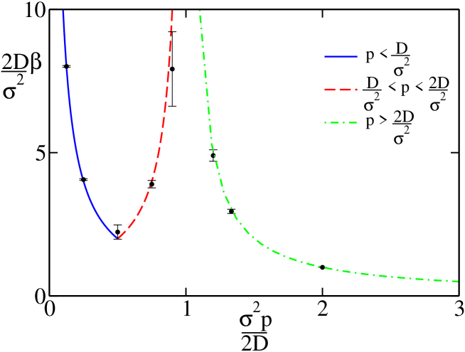
Figure 1:

Figure 2:

References

- (1) S. Dietrich, in Phase Transitions and Critical Phenomena, edited by C. Domb and J. Lebowitz (Academic Press, New York, 1983), Vol. 12; D.E. Sullivan and M.M. Telo da Gama, in Fluid Interfacial Phenomena, edited by C.A. Croxton (Wiley, New York, 1986).
- (2) K. Binder, D. Landau, and M. Müller, J. Stat. Phys. 110, 1411 (2003).
- (3) M. Kardar, G. Parisi, and Y. -C. Zhang, Phys. Rev. Lett. 56, 889 (1986); T. Halpin-Healy and Y.-C. Zhang, Phys. Rep. 254, 215 (1995); J. Krug, Adv. Phys. 46, 139 (1997).
- (4) H. Hinrichsen, R. Livi, D. Mukamel, and A. Politi, Phys. Rev. Lett. 79, 2710 (1997); Y. Tu, G. Grinstein, and M.A. Muñoz, ibid. 78, 274 (1997); M.A. Muñoz and T. Hwa, Europhys. Lett. 41, 147 (1998); W. Genovese and M.A. Muñoz, Phys. Rev. E 60, 69 (1999); F. de los Santos, M.M. Telo da Gama, and M.A. Muñoz, Europhys. Lett. 57, 803 (2002).
- (5) M.A. Muñoz, in Advances in Condensed Matter and Statistical Mechanics, edited E. Korutcheva and R. Cuerno (Nova Science Publishers, New York, 2004), p. 37; F. de los Santos and M.M. Telo da Gama, Trends Stat. Phys. Vol. 4, 61 (2004).
- (6) M. A. Muñoz, F. de los Santos, and A. Achahbar, Braz. J. Phys. 33, 443 (2003);
- (7) T. Kissinger, S. Kotowicz, O. Kurz, F. Ginelli, and H. Hinrichsen, J. Stat. Mech.: Theor. Exp. 2005, P06002.
- (8) O. Al Hammal, F. de los Santos, and M. A. Muñoz, J. Stat. Mech.: Theor. Exp. 2005, P10013.
- (9) C. Van den Broeck, J. M. R. Parrondo, J. Armero, and A. Hernández-Machado, Phys. Rev. E 49, 2639 (1994); M.G. Zimmermann, R. Toral, O. Piro, and M. San Miguel Phys. Rev. Lett. 85, 3612 (2000).
- (10) T. Birner, K. Lippert, R. Müller, A. Kühnel, and U. Behn, Phys. Rev. E 65, 046110 (2002).
- (11) I.S. Gradshteyn and I.M. Ryzhik, Table of Integrals, Series and Products, Academic Press 1988.
- (12) N.G. van Kampen, Stochastic Processes in Physics and Chemistry, (North Holland, Amsterdam 1992).
- (13) A. Elbert and M.E. Muldoon, Proc. Roy. Soc. Edin. 129A, 57 (1999).
- (14) M.A. Muñoz, F. Colaiori, and C. Castellano, Phys. Rev. E 72, 056102 (2005).