Limitations for the determination of piezoelectric constants
with piezoresponse force microscopy

Abstract

At first sight piezoresponse force microscopy (PFM) seems an ideal technique for the determination of piezoelectric coefficients (PCs), thus making use of its ultra-high vertical resolution ($<$ 0.1 pm/V). Christman et al. Chr98 first used PFM for this purpose. Their measurements, however, yielded only reasonable results of unsatisfactory accuracy, amongst others caused by an incorrect calibration of the setup. In this contribution a reliable calibration procedure is given followed by a careful analysis of the encounted difficulties determining PCs with PFM. We point out different approaches for their solution and expose why, without an extensive effort, those difficulties can not be circumvented.

The determination of the magnitude of the piezoelectric coefficients (PCs) is still a rewarding experimental challenge. Although several methods have been utilized (measuring the resonance frequencies of specifically cut samples Ogi02 , determining the velocity of sound Kov90 , utilizing a Berlincourt meter Zha97 or using optical heterodyne interferometry Roy92 ), they all suffer from being cumbersome and the published values vary strongly. In the past years piezoresponse force microscopy (PFM) has become a standard tool for investigating ferroelectric and thus piezoelectric samples New making use of the converse piezoelectric effect. A detailed description of PFM can be found elsewhere Alexe ; Jun06a . However, despite its ultra-high vertical resolution in the sub-picometer regime, it is not applied for the precise determination of PCs. This is mainly due to the fact, that even well established PCs could not be reliably confirmed with PFM. Interestingly, the failure of PFM measurements with high quantitative accuracy is mostly due to the incorrect calibration the instrument. However, even with appropriate calibration, PFM is not capable of determining piezoelectric coefficients.

In this contribution, we will show why the calibration technique generally referred to Chr98 leads to wrong PFM-calibration constants. We will in return present a reliable calibration procedure. We will further more focus on the difficulties to determine PCs with high accuracy with PFM. It will unfortunately turn-out that a precise determination of PCs with PFM is generally not possible.

Piezoresponse force microscopy is based on the deformation of the sample due to the converse piezoelectric effect. The PFM is a scanning force microscope (SFM) operated in contact mode with an alternating voltage $U_{\rm tip}$ applied to the tip. In piezoelectric samples this voltage causes thickness changes $\Delta t$ and therefore vibrations of the surface which lead to oscillations of the cantilever that can be read out with a lock-in amplifier. In order to obviate misunderstandings we briefly define the symbols used later on for the outputs of the lock-in amplifier (LI). A LI-signal can generally be described in a circular coordinate system as a vector $\bf P$ with an appropriate length $P$ and an angle $\theta$ with respect to the reference signal. This is the way the signals are read-out from a single-phase LI. In case of a dual-phase LI, the two output signals can optionally also be displayed in a cartesian coordinate system thus resulting in the output signals $P^{X}$ and $P^{Y}$. Note that adjusting the phase $\phi$ of the reference signal corresponds to a rotation of the coordinate system. In the following we will adapt the usual notation naming the output signals $P$ and $\theta$ ($\phi=0$) of the LI the PFM-signals, subscripts specify the particular sample.

In general the calibration of the SFM for PFM-measurements is performed according to the hence often cited work by Christman et al. Chr98 . In brief, a piezoelectric sample with known PC is brought into the PFM-setup. Due to its very precisely determined PC an $\alpha$-quartz-plate ($d_{11}=2.3\pm 0.05$ pm/V Lan ) is generally used for this purpose. One presumes thus to obtain the relation between the PFM-signal $P_{\alpha}$ and the vibration amplitude $\Delta t=d_{11}\,U_{\rm tip}$ of the surface, leading to a PFM-calibration constant $k_{\rm PFM}=\Delta t/P_{\alpha}=d_{11}\,U_{\rm tip}/P_{\alpha}$. Thus by measuring $P$ of any other sample one presumes to determine its particular PC as

$$d=k_{\rm PFM}\,P/U_{\rm tip}=d_{11}P/P_{\alpha}\quad.$$ (1)

However, due to the system-inherent background Jun06a this calibration procedure and thus the precise determination of PCs fails. This background, present in current SFM setups, shows-up as a frequency dependent contribution to the PFM-signal, probably caused by a wealth of mechanical resonances of the SFM-head. The amplitude of the background (1–10 pm/V) scales linearly with $U_{\rm tip}$, its phase varies randomly. Possible consequences of the background-adulterated PFM-signals have been presented in detail elsewhere Jun07b . Hitherto attempts to suppress the background by modification of the SFM-head failed.

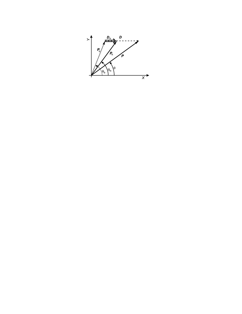
Figure 1: Output signals of the lock-in amplifier in the $X$-$Y$-plane. The system-inherent background is ${\bf P}_{b}$. A piezoelectric standard sample with a piezoelectric coefficient $d_{\alpha}$ contributes ${\bf D}_{\alpha}$ $(\Rightarrow)$ to the resulting PFM-signal $\bf P_{\alpha}$. Same applies for the sample with the PC to be measured: it’s contribution to the measured signal $\bf P$ is $\bf D$ $(\dashrightarrow)$.

Figure 1 depicts the situation showing PFM-signals in a vectorial diagram. Note that $\bf D_{\alpha}$ denotes the contribution of the calibration sample to the PFM-signal which should not be confused with its piezoelectric coefficient $d_{\alpha}$. For the sample to be measured the same notation ($\bf D$ and $d$) applies. Starting from scratch: the background ${\bf P}_{b}$ results in PFM-signals of $P_{b}$ and $\theta_{b}$. The contribution of the calibration sample adds on the background as ${\bf P}_{\alpha}={\bf P}_{b}+\bf D_{\alpha}$ thus resulting in the PFM-signals $P_{\alpha}$ and $\theta_{\alpha}$. The sample to be measured finally leads to the PFM-signals $P$ and $\theta$. From simple geometrical considerations is can be seen that

$$P_{\alpha}=\sqrt{P_{b}^{2}+D_{\alpha}^{2}+2P_{b}D_{\alpha}\cos\theta_{b}}\quad.$$ (2)

The same expression applies for $P$ substituting $D_{\alpha}$ by $D$. It is now self-evident that because ${\bf P}_{b}\neq 0$ and thus $\bf P_{\alpha}\neq D_{\alpha}$ the procedure described previously for calibrating the PFM and consequently the determination of $d$ fails.

An example shows the significance of the situation described above. In Fig. 1 the different contributions to the PFM-signals are shown in realistic proportions when using $\alpha$-quartz ($d_{11}=2.3$ pm/V) for calibration. Let us assume the background to have an amplitude of $P_{b}=8$ pm/V at an angle of $\theta_{b}=60^{\circ}$ and the sample to have a PC of $d=7$ pm/V. Using Eqs 1 and 2 would lead to $d=d_{11}\,P/P_{\alpha}\simeq 3.2$ pm/V which is wrong by a factor of more than two.

To overcome the above mentioned difficulties it is essential to conduct a reliable calibration of the PFM. Therefore three steps have to be accomplished:

• Calibration of the z-scanner of the SFM. This can be accomplished with a height standard.

• Determination of thickness change $\Delta t$ of the calibration sample at a specific voltage $U_{\rm tip}$ and frequency $f$ applied to the tip. This measurement is performed with the ”height-modus” of the SFM. Therefore a piezoceramic sample with a large PC ($\sim 500$ pm/V) is most appropriate. The frequency $f$ must be low with respect to the feedback loop of the SFM thus the z-scanner can fully follow the movement ($f\sim 0.1$ – 1 kHz).

  The PC of the calibration sample has to be large in order to yield measurable thickness changes $\Delta t$ at moderate voltages. Applying e.g. $10\,$V_pp to the tip for a sample with a PC of 500 pm/V results in a thickness change of $\Delta t_{\rm PZT}=5\,$nm, easily detectable with SFM. Note that $\alpha$-quartz is not suited as it would only give $\Delta t=$0.023 nm. This, however, is not measurable with the ”height-modus” of the SFM.

• With the piezoceramic sample used in the step before, using the same voltage and the same frequency applied to the tip the PFM can now be calibrated just by disabeling the feedback-loop and measuring the output $P_{\rm PZT}$ of the lock-in amplifier. One thus gets the wanted calibration constant $k_{\rm PFM}=\Delta t_{\rm PZT}/P_{\rm PZT}$.

Another possibility to calibrate the SFM by determining the detector sensitivity via a force-distance measurement and then calculating the expected PFM-signal Har . This calibration method has a disadvantage since it is a low-frequency measurement whereas for PFM usually frequencies in the kHz regime are used. It is thus not performed under the same conditions than the PFM measurements.

Now, after calibration of the PFM, the main problem for determining reliable PCs with the PFM remains the background. Although the origin of the background is not fully understood, it can be attributed to resonances of the whole SFM setup, i.e. head of the microscope, and sample & sample stage, depending on the specific realization of the top electrode. Therefore two situations have to be discussed individually: (a) the tip and (b) a large area metallization acting as top electrode. In both cases the backside of the sample is covered with a large area electrode (Fig. 2).

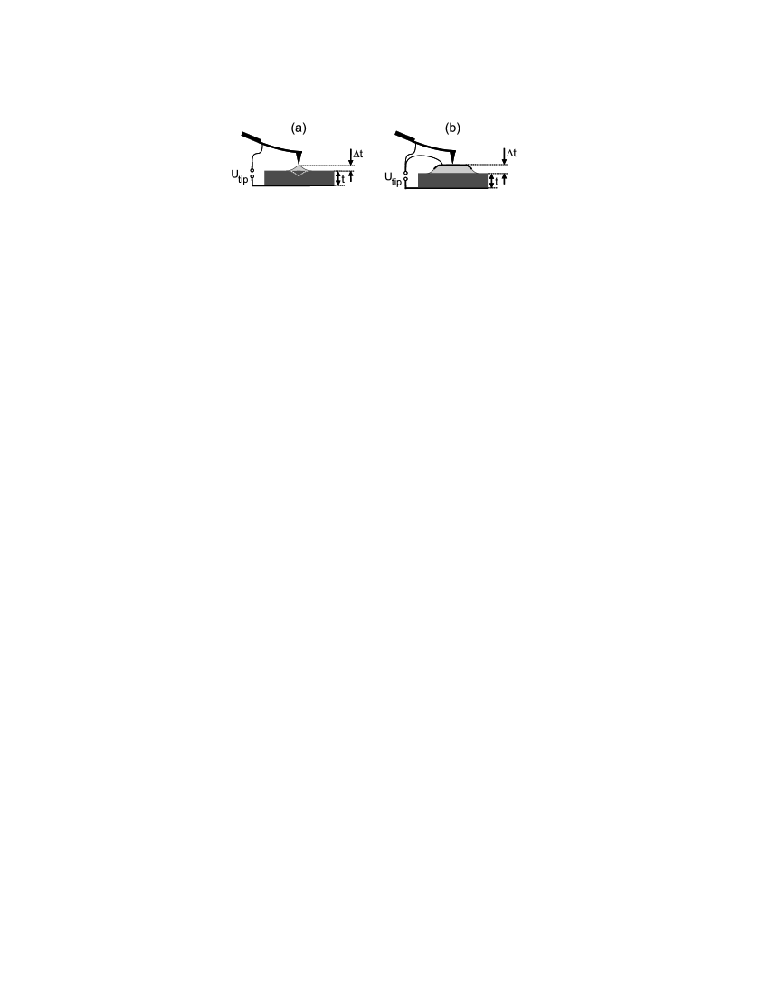
Figure 2: (a) The tip acting as electrode. Only a very small volume of the sample (some µm³) contributes to the deformation. (b) A large area top electrode. Beneath the central part of the electrode, the whole volume of the sample expands homogeneously. Near the edges clamping influences the deformation.

Tip as electrode. This is the standard configuration for PFM-measurements yielding a high lateral resolution. In this situation, the electric field inside the crystal can reach values of up to $E\approx 10^{9}$ V/m just underneath the tip, depending on the tip radius and the dielectric constant of the sample. However, due to the strong inhomogeneity caused by the sharp tip, $E$ decays within $\leq 1\,\mu$m inside the sample Ott04 . The piezoelectrically excited region is thus only a few µ$\rm m^{3}$(Fig. 2(a)). This has two important consequences on PFM-imaging: (i) the whole sample is at rest, the background is only due to the SFM-head (incl. cantilever) and can thus be determined e.g. with a glass plate Jun06a ; (ii) Due to clamping of the surrounding material the crystals deformation is drastically reduced. The values measured in this way were found to be too small by a factor of up to three Jun07a . As a result measurements with the tip acting as electrode are not suited for the determination of PCs with high accuracy.

Large area electrode. To avoid the problem of clamping and to minimize any effect of electrostatic interaction between the cantilever and the sample, a large area electrode of some mm² is evaporated on top of the sample. Electrical contact is performed directly to the electrode through an external wire, short-circuited with the tip (Fig. 2(b)). Besides being unclamped in the center of the electrode, this configuration offers another advantage in comparison to the situation with the tip acting as electrode: The electrical field applied to the crystal is well defined as it is homogeneous across the whole sample thickness. In this configuration, however, the background is no longer independent of the sample which turns out to be a probably irresolvable drawback. Since the whole sample is piezoelectrically excited, sample and sample-holder also contribute to the background. A series of experiments with different fixations of the sample (sticking it with epoxy on a large lead block, embedding it in rubber, or suspending it freely) failed. Every mounting showed its own frequency dependence of the PFM-signal why a determination of the background is not possible. Thus, measurements with the large area electrodes are not suited for the determination of PCs with high accuracy.

Of course the immediate question arises whether there is any possibility to circumvent the drawbacks presented above, thus enabling a precise determination of piezoelectric coefficients. A reliable measurement of PCs with the tip acting as electrode can be excluded as it fails due to clamping, i.e., a fundamental physical reason. For the measurements using large top electrodes, however, the situation is different since so far technical deficiencies cause the failure. In the following we will discuss three approaches that might overcome the difficulties mentioned above.

(1) In principle, one can think about a SFM-setup suppressing any kind of background. Although difficult to realize, it is not impossible. As a reminder the amplitude of the background is of the order of 10 pm/V, which, using standard PFM settings (10 V applied to the tip) becomes comparable to the radius of an atom. The same scale applies for the PCs to be measured. Obviously the specific SFM we used (SMENA from NT-MDT) is not of low quality but lock-in detection is amazingly sensitive. Note that in order to become interesting for the determination of PCs, the background needs to be reduced at least by two (!) orders of magnitude. Taking this into account, building a ”background-free” SFM appears as a remarkably serious challenge.

(2) Another approach to circumvent the background-problem is based on multi-domain samples. Measuring the PFM-signals on both domain faces (with the same background) would automatically yield the correct PC of the sample Jun06a . Apparently straightforward, this approach results in new troubles: the clamping between adjacent domains. As expected from theoretical considerations, and verified experimentally Jun07c , the surface deformation is affected on a length scale similar to the thickness of the sample. Thus, for a 500 µm thick sample, reliable values for the piezomechanical deformation can only be obtained at a distance of $>500$ µm from any domain boundary. As a first consequence, the use of a large bi-domain sample is required. Furthermore, the sample has to be transferred by more than 1 mm for measuring reasonable PFM-signals on both domain faces. Unfortunately, when performing such crucial changes in the mechanical setup, the background can not be presumed to remain unchanged. This, however, is an absolute condition for the quantitative analysis of a multi-domain measurement as proposed here. Even worse, there is no way to find-out, whether the translation of the sample did affect the background or not.

One could think, of course, to reduce this difficulty using thinner crystals, e.g., 50 µm thickness, thus scaling the problems described above by one order of magnitude. But also a 100 µm translation is still too much. Since for this measurement, the samples must be free-standing, to make them even thinner is not trivial. Thus although seemingly easy, this approach also suffers a series of drawbacks not yet resolved.

(3) Finally, and so far the only realizable solution to the problems described above consists of using very particular settings for the PFM, avoiding the contribution of the background by applying frequencies of $\ll 1$ Hz to the tip, thus excluding the resonances of the setup. This requires of course to disable the feedback of the SFM. Due to the very long integration time of several minutes, necessary for obtaining reliable data, those measurements can only be carried out when the environment of the setup is at quiet as possible. Although this measurement scheme might provide the best data for PCs when using PFM, it is not a detection method suitable to provide reliable values of high accuracy due to inherent drift and noise in current SFM setups.

In this contribution, we extensively discussed the capability of piezoresponse force microscopy (PFM) to provide accurate values for the piezoelectric coefficients (PCs) of single crystals. We first presented a calibration procedure for PFM measurements. In the following we carried out a careful analysis of the different measurement techniques and the belonging drawbacks. It turned out that without an extensive effort PFM is not suited to yield reliable PCs.

Acknowledgments

We thank David Scrymgeour for helpful discussions. Financial support of the DFG research unit 557 and of the Deutsche Telekom AG is gratefully acknowledged.

References

- (1) J. A. Christman, J. R. R. Woolcott, A. I. Kingon, and R. J. Nemanich, Appl. Phys. Lett. 73, 3851 (1998)
- (2) H. Ogi, Y. Kawasaki, M. Hirao, and H. Ledbetter, J. Appl. Phys. 92, 2451(2002).
- (3) G. Kovacs, M. Anhorn, H. E. Engan, G. Visintini, and C. C. W. Ruppel, IEEE Ultrasononics Symposium 435 (1990).
- (4) Z. Zhao, H. L. Chan, and C. L. Choy, Ferroelectrics 195, 35 (1997).
- (5) D. Royer and V. Kmetik, Electron. Lett. 28, 1828 (1992).
- (6) R. E. Newnham Properties of Materials (Oxford University Press, New York, 2005)
- (7) M. Alexe and A. Gruverman, eds., Nanoscale Characterisation of Ferroelectric Materials (Springer, Berlin; New York, 2004) 1st ed.
- (8) T. Jungk, A. Hoffmann, and E. Soergel, Appl. Phys. Lett. 89, 163507 (2006).
- (9) T. Jungk, A. Hoffmann, and E. Soergel, submitted (2007).
- (10) Landolt-Börnstein III/29 (Springer, Berlin; New York, 1979)
- (11) C. Harnagea and A. Pignolet in Nanoscale Characterisation of Ferroelectric Materials, M. Alexe and A. Gruverman, eds., Chap. 2 (Springer, Berlin; New York, 2004) 1st ed.
- (12) T.Otto, S. Grafström, and L. Eng, Ferroelectrics 303, 149 (2004)
- (13) T. Jungk, A. Hoffmann, and E. Soergel, Appl. Phys. A 86, 353 (2007).
- (14) T. Jungk, A. Hoffmann, and E. Soergel, submitted (2007).