Conductance of a quantum point contact based on spin-density-functional theory

Abstract

We present full quantum mechanical conductance calculations of a quantum point contact (QPC) performed in the framework of the density functional theory (DFT) in the local spin-density approximation (LDA). We start from a lithographical layout of the device and the whole structure, including semi-infinitive leads, is treated on the same footing (i.e. the electron-electron interaction is accounted for in both the leads as well as in the central device region). We show that a spin-degeneracy of the conductance channels is lifted and the total conductance exhibits a broad plateau-like feature at $\sim 0.5\times 2e^{2}/h$. The lifting of the spin-degeneracy is a generic feature of all studied QPC structures (both very short and very long ones; with the lengths in the range $40\lesssim l\lesssim 500$ nm). The calculated conductance also shows a hysteresis for forward- and backward sweeps of the gate voltage. These features in the conductance can be traced to the formation of weakly coupled quasi-bound states (magnetic impurities) inside the QPC (also predicted in previous DFT-based studies). A comparison of obtained results with the experimental data shows however, that while the spin-DFT based ”first-principle” calculations exhibits the spin polarization in the QPC, the calculated conductance clearly does not reproduce the 0.7 anomaly observed in almost all QPCs of various geometries. We critically examine major features of the standard DFT-based approach to the conductance calculations and argue that its inability to reproduce the 0.7 anomaly might be related to the infamous derivative discontinuity problem of the DFT leading to spurious self-interaction errors not corrected in the standard LDA. Our results indicate that the formation of the magnetic impurities in the QPC might be an artefact of the LDA when localization of charge is expected to occur. We thus argue that an accurate description of the QPC structure would require approaches that go beyond the standard DFT+LDA schemes.

I Introduction

Experimental evidence of an additional $0.7\times 2e^{2}/h$ conductance feature in quantum point contacts (QPCs)Thomas1996 ; Thomas1998 ; trench-etchedQPC ; epitaxQPC ; Reillytwin ; Cronenwett ; Reilly_2002 ; Reilly_2005 ; Graham ; Rokhinson has generated enormous theoretical activity during recent decadeCronenwett ; Reilly_2002 ; Reilly_2005 ; Berggren ; Starikov ; Jaksch ; Havu ; Meir_2002 ; Meir_2003 ; Meir_Nature ; Shelykh . While a usual conductance quantization in terms of $2e^{2}/h$ can be successfully explained in a one-electron pictureWharam , no consensus on the origin of the 0.7 anomaly has been reached so far. Experimental data, based on magnetic field dependence of the plateau positionThomas1996 ; Thomas1998 and observation of the zero bias anomalyCronenwett clearly point out at spin origin of this effect. The spin origin was adopted in many theories which include, just to name a few of them, a spontaneous spin-polarization inside the constriction of the QPC originated from the exchange-correlation interactionBerggren ; Starikov ; Jaksch ; Havu , the ferromagnetic-antiferromagnetic exchange interaction with a large localized spinShelykh , a formation of polarized quasi-bound states and Kondo effectMeir_2002 ; Meir_2003 , as well as several others. However, none of the existing theories reproduce quantitatively the 0.7 conductance anomaly observed in almost all QPCsThomas1996 ; Thomas1998 ; trench-etchedQPC ; epitaxQPC ; Reillytwin ; Cronenwett ; Reilly_2002 ; Reilly_2005 . Note that some of approaches based on phenomenological models do recover the 0.7 feature in the conductanceReilly_2002 ; Reilly_2005 ; Bruus . Such the approaches, while providing an important insight for an interpretation of the experiment, are not, however, able to uncover the microscopic origin on the observed effect.

A powerful technique capable of providing detailed information about electronic and transport properties on the microscopic level is based on the ”first principle” density functional theory (DFT) approach. The spin DFT calculations addressing the 0.7 anomaly in the QPC have been presented by various groupsBerggren ; Starikov ; Jaksch ; Havu ; Meir_2002 ; Meir_Nature . However, many of these calculations show rather conflicting results. For example. Refs. Meir_2002, ; Meir_2003, ; Meir_Nature, attribute the 0.7 anomaly to formation of the localized magnetic moment in the QPC, whereas such quasi-bound states are not recovered in Refs. Berggren, ; Starikov, ; Jaksch, ; Havu, . In contrast, Ref. Starikov, relates the $0.7$ anomaly to multiple metastable spin-polarized solutions. The recent study of Jaksch et al.Jaksch suggests that the spin polarization is absent in short QPCs and is increased with the increase of the length of the QCP. This seems to contradict the results reported by Rejec and MeirMeir_Nature who find that a strong spin polarization due to the magnetic impurity formation is a generic feature seen in short as well as in long QPCs.

Motivated by the above mentioned conflicting results and conclusions, in this paper we perform “first principle” full quantum mechanical transport calculations of the conductance of the QPC based on the spin DFT in the local spin-density approximation (LDA). [We use a notation “first principle” in a sense that we start from a lithographical geometry of the gates and a heterostructure layout]. The main features of our calculations and the relation of our model to the DFT-based calculations reported previously are as follow. In the present paper the QPC is viewed as an inherently open system where the solution of the Schrödinger equation consists of continuous scattering states. This is in contrast to Refs. Berggren, ; Jaksch, treating a QPC as a closed system where the solution of the Schrodinger equation is represented by a discrete set of the eigenfunctions. In our calculations we start from a lithographical layout of the device, which is in contrast to Ref. Havu, using a simplified model of an external confinement potential. (Note that importance of an accurate treatment of the confinement potential is stressed in Ref. Reilly_2005, , where the phenomenology and experimental data indicate that the 0.7 feature depends strongly on the potential profile of the contact region). Our model (but not the computational technique) is conceptually similar to the one used by Rejec and MeirMeir_Nature (see also Ref. Meir_2002, reporting similar findings) where a QPC is treated as an open structure and where a realistic model for the external confinement potential due to metallic gates is utilized. In their study Rejec and Meir focus on the calculation of the electron density, predicting the formation of a localized spin-degenerate quasi-bound state (magnetic impurity). They did not, however, perform transport conductance calculations so the central question whether the 0.7-anomaly is indeed related to the formation of a magnetic impurity has remained unanswered. In the present paper we hence focus on the calculation of the spin-resolved conductance of the quantum point contact.

The details of our model and the Hamiltonian are given in Sec. II. In Sec. III we present our method for the calculation of the electron density and conductance which is based on the self-consistent Greens function technique combined with the spin DFT in the local spin density approximation. This method is a generalization of a method of Ref. opendot, for the case of spin. The results are presented in Sec. IV. Our calculations reconfirm the finding reported by Rejec and MeirMeir_Nature concerning the formation of the localized spin-degenerate quasi-bound states (magnetic impurities) within the DFT+LDA approach. However, the calculated conductance clearly does not reproduce the 0.7 anomaly observed in almost all QPCs of various geometries. Instead, the total conductance shows a broad feature peaked at $0.5\times 2e^{2}/h$. A similar feature is also present in the range of the gate voltages where a second step in the conductance develops. The calculated conductance also shows a hysteresis for forward- and backward sweeps of the magnetic fields. (We stress that all these results are generic; we studied QPS with lengths in the range 40 - 500 nm and electron densities in the leads in the range $10^{15}\text{m}^{-2}-4\cdot 10^{15}\text{m}^{-2}$, with very similar results). In Sec. V we discuss the obtained results and critically examine the DFT+LDA-based conductance calculations. We suggest that the failure of the DFT+LDA approach to reproduce quantitatively the 0.7 anomaly may be due to the lack of the derivative discontinuity in the standard LDA approximation (leading to uncorrected self-interaction errors) for the case when localization of charge is expected to occur, so that the magnetic impurity formation may be an artefact of the DFT+LDA approach due to the spurious self-interaction.

II Model

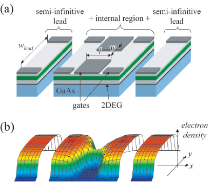
Figure 1: (color online) (a) Structure of a quantum point contact typically fabricated by a split-gate technique. An internal computational region is attached to two semi-infinite leads which serve as electron reservoirs. The gates of the quantum point contact form a constriction of the length $l$ and the width $w$; $w_{lead}$ is the distance between the gates defining the leads. (b) A representative calculated electron density.

We consider a quantum point contact (QPC) placed between two semi-infinite electron reservoirs. A schematic layout of the device is illustrated in Fig. 1(a). Charge carriers originating from a fully ionized donor layer form the two-dimensional electron gas (2DEG) which is buried inside a substrate at the GaAs/Al_xGa_1-xAs heterointerface at the distance $b$ from the surface. Metallic gates are situated on the top of the heterostructure and define the quantum point contact as well as electron reservoirs that are are represented by uniform quantum wires of the infinite length.

The Hamiltonian of the whole system (QPC + leads) within the Kohn-Sham formalism can be written in the form $H=\sum_{\sigma}H^{\sigma},$

$$H^{\sigma}=-\frac{\hbar^{2}}{2m^{\ast}}\nabla^{2}+V^{\sigma}(\mathbf{r}),$$ (1)

$\mathbf{r}=(x,y)$, $m^{\ast}=0.067m_{e}$ is the GaAs effective mass and $\sigma$ stands for spin-up, $\uparrow$, and spin-down, $\downarrow$, electrons. The first term in (1) is the kinetic energy of an electron while $V^{\sigma}(\mathbf{r})=V_{conf}(\mathbf{r})+V_{H}(\mathbf{r})+V_{xc}^{\sigma}(\mathbf{r})$ is the total confining potential which is a sum of the electrostatic confinement potential, the Hartree potential, and the exchange-correlation potential, respectively. The electrostatic confinement $V_{conf}(\mathbf{r})=V_{gates}(\mathbf{r})+V_{donors}+V_{Schottky}$ includes contributions from the top gates, the donor layer and the Schottky barrier. The explicit expressions for the potentials $V_{gates}(\mathbf{r})$ and $V_{donors}$ are given in Refs. Davies_gate, and Martorell_donor, ; the Schottky barrier is chosen to be $V_{Schottky}=0.8$ eV. The Hartree potential is written in a standard form

$$V_{H}(\mathbf{r})=\frac{e^{2}}{4\pi\varepsilon_{0}\varepsilon_{r}}\int d\mathbf{r}\,^{\prime}n(\mathbf{r}^{\prime})\left(\frac{1}{|\mathbf{r}-\mathbf{r}^{\prime}|}-\frac{1}{\sqrt{|\mathbf{r}-\mathbf{r}^{\prime}|^{2}+4b^{2}}}\right),$$ (2)

where $n(\mathbf{r})=\sum_{\sigma}n^{\sigma}(\mathbf{r})$ is the total electron density and the second term describes the mirror charges placed at the distance $b$ from the surface, $\varepsilon_{r}=12.9$ is the dielectric constant of GaAs, and the integration is performed over the whole device area including the semi-infinite leads.

The exchange-correlation potential $V_{xc}^{\sigma}(\mathbf{r})$ in the local spin density approximation is given by the functional derivative Giuliani_Vignale

$$V_{xc}^{\sigma}=\frac{d}{dn^{\sigma}}\left\{n\epsilon_{xc}\left(n\right)\right\}.$$ (3)

For $\epsilon_{xc}$ we have employed two commonly used parameterizations, by Tanatar and CeperleyTC and by Attacalite et alAMGB . These two parameterizations give very similar results. All the results presented below correspond to the parameterization of Tanatar and CeperleyTC .

III Method

The central quantity in transport calculations is the conductance. In the linear response regime, it is given by the Landauer formula $G=\sum_{\sigma}G^{\sigma}$, Datta_book

$$G^{\sigma}=-\frac{e^{2}}{h}\int dE\,T^{\sigma}(E)\frac{\partial f\left(E-E_{F}\right)}{\partial E},$$ (4)

where $T^{\sigma}(E)$ is the total transmission coefficient for the spin channel $\sigma$, $f(E-E_{F})$ is the Fermi-Dirac distribution function and $E_{F}$ is the Fermi energy. In order to calculate $T^{\sigma}(E)$ we use the method developed in Ref. opendot, for the spinless electrons and generalize it here for the presence of two spin channels. For the case of completeness, the main steps of our calculations are presented below.

We discretize Eq. (1) and introduce the tight-binding Hamiltonian with the lattice constant of $a=4$ nm. (Such a small $a$ ensures that the tight-binding Hamiltonian is equivalent to the continuous Schrödinger equation.) The retarded Green’s function is introduced in a standard wayDatta_book ,

$$\mathcal{G}^{\sigma}=\left(E-H^{\sigma}+i\eta\right)^{-1}.$$ (5)

The Green’s function in the real space representation, $\mathcal{G}^{\sigma}(\mathbf{r},\mathbf{r},E)$, provides an information about the electron density at the site $\mathbf{r},$ Datta_book

$$n^{\sigma}(\mathbf{r})=-\frac{1}{\pi}\Im\int dE\,\mathcal{G}^{\sigma}(\mathbf{r},\mathbf{r},E)\,f(E-E_{F}).$$ (6)

Note that $\mathcal{G}^{\sigma}(\mathbf{r},\mathbf{r},E)$ is a rapidly varying function of energy. As a result, a direct integration along the real axis in Eq. (6) is rather ineffective as its numerical accuracy is not sufficient to achieve a convergence of the self-consistent electron density. Because of this, we transform the integration contour into the complex plane $\Im[E]>0,$ where the Green’s function is much more smoother (see Ref. opendot, for details).

In order to calculate the Green’s function of the whole system (QPC + leads) we divide it into three parts, the internal region and two semi-infinite leads, as shown in Fig. 1(a). The internal region consists of the QPC as well as a part of the leads. In order to link the internal region and the leads together the self-consistent charge density (and the potential) at both sides must be the same. To fulfill this requirement, we place the semi-infinite leads far away from the central region so that the gates defining the QPC do not affect the electron density distribution in the leads. (The distribution is determined solely by the lead gate voltage, see Fig. 1.) As a result, it is fully justified to approximate the semi-infinitive leads by a uniform quantum wire. The self-consistent solution for the latter can be found by the technique developed in Ref. Ihnatsenka, . Eventually, the Green’s function of the whole system is calculated by linking the surface Green’s function for the semi-infinite leads (calculated using the technique of Ref. Ihnatsenka, ) and the Green’s function of the internal region with the help of the the Dyson equationZozoulenko_1996 .

All the calculations described above are performed self-consistently in an iterative way until a converged solution for the electron density and potential (and hence for the total Green’s function) is obtained. Having calculated the total self-consistent Green’s function, the scattering problem is solved where the scattering states in the leads (both propagating and evanescent) are obtained using the Green’s function technique of Ref. Ihnatsenka, .

Having calculated the Green’s function we can find the local density of states (LDOS) in the QPCDatta_book

$$\text{LDOS}^{\sigma}(x,E)=-\frac{1}{\pi}\Im\int dy\;\mathcal{G}^{\sigma}(x,y,E).$$ (7)

The self-consistent solution in quantum transport or electronic structure calculations is often found using a “simple mixing” method. It is the most robust and reliable algorithm with only one disadvantage, namely a low convergence rate. The charge density on the ( $i+1$)-th iteration loop is updated through the input $n_{i}^{in}(\mathbf{r})$ and output $n_{i}^{out}(\mathbf{r})$ densities on the previous $i$-th iteration

$$n_{i+1}^{in}(\mathbf{r})=(1-\epsilon)n_{i}^{in}(\mathbf{r})+\epsilon\,n_{i}^{out}(\mathbf{r}),$$ (8)

with $\epsilon$ being a small constant $\sim 0.1-0.01$. It is typically needed $\sim 200-2000$ iteration steps to achieve our convergence criterium for the relative density update on the $i$-th iteration step,

$$\frac{|n_{i}^{out}-n_{i}^{in}|}{n_{i}^{out}+n_{i}^{in}}<10^{-7},$$ (9)

where $n=\int n(\mathbf{r})\,d\mathbf{r}$ is the total electron number in the internal region during the $i$-th iteration step.

In order to trigger a spin-polarized solution we apply at early iterations a small parallel magnetic field, $B=0.05$ T. The final solution is driven mostly by the exchange interaction which is about four orders of magnitude larger that the Zeeman energy at $B=0.05$ T.

The self-consistent calculation are performed for different gate voltages. To facilitate the calculations we use a solution from the previous value of the gate voltage as an initial guess for the subsequent one. It is worth noting that the modified Broyden’s second methodSingh , which can greatly reduce the number of iterations for the case of spinless electronsopendot , does not lead to reliable convergent results for the case of the spin degree of freedom.

IV Results

We calculate the conductance of a split-gate QPC with following parameters representative for a typical experimental structure. The 2DEG is buried at $b=70$ nm below the surface (the widths of the cap, donor and spacer layers are 24 nm, 36 nm and 10 nm respectively), the donor concentration is $0.6\cdot 10^{24}$ m^-3. The width of the semi-infinitive leads is $w_{lead}=400$ nm, and the width of the QPC constriction is $w=100$ nm, see Fig. 1 (a). The width $w$ is kept constant throughout the paper, while the length is varied in the range $l=40-500$ nm. The gate voltage applied to the gates defining the leads is $V_{lead}=-0.73$ V. With these parameters of the device there are 18 spin-up and 18 spin-down channels available for propagation in the leads and the electron density in the center of the leads is $n_{lead}^{\uparrow}=n_{lead}^{\downarrow}=2.2\cdot 10^{15}$ m^-2. Such a large number of the channels in the leads makes its DOS to mimic a smooth DOS of the two-dimensional electron gas. The temperature is fixed at $T=0.2$ K for all results presented below.

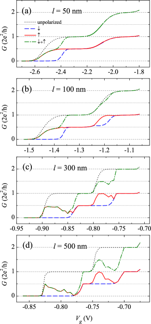
Figure 2: (color online) Conductance of the quantum point contact of different lengths $50<l<500$ nm as a function of the gate voltage $V_{g}$. The geometrical width of the constriction is $w=100$ nm; the geometrical length $l$ is indicated in the figures. The dashed line corresponds to the spin-unpolarized solution.

Figure 2 shows the conductance of QPCs of different constriction lengths $l$ ranging from $l=50$ nm (a very short QPC) to $l=500$ nm (a long quantum wire-type QPC). The conductance of all QPCs shows a broad plateau-like feature at $0.5\times 2e^{2}/h$. As the length of the constriction increases, a dip following 0.5-plateau starts to develop in the QPC conductance. An inspection of the spin-resolved conductance demonstrates that 0.5 feature corresponds to the transmission of only one spin channel (say, spin-up), whereas the second (spin-down) conductance channel is totally suppressed. For long constrictions ($l\gtrsim 300$ nm) the 0.5 plateau starts to “wear down” transforming into a broad feature whose maximal amplitude is less than $0.5\times 2e^{2}/h$. If the constriction is sufficiently long ($l\gtrsim 100$ nm), a conductance plateau at $\sim 1.5\times 2e^{2}/h$ starts to develop and a conductance dip following the 1.5-plateau also starts to emerge as the length of the constriction increases.

To shed light on a microscopic origin of the $0.5\times 2e^{2}/h$ conductance feature and the suppression of the spin-down channel let us inspect the charge density and energy structure of the QPC.

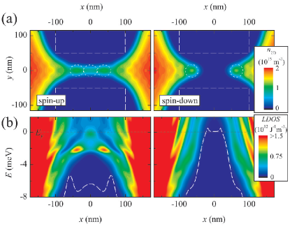
Figure 3: (color online) Formation of quasi-bound states in the quantum point contact. (a) The charge density and (b) the local density of states are shown for the regime of one transmitted spin-up and totally blocked spin-down channel. The left and right columns correspond to spin-up and spin down electrons. The white dashed lines in (b) indicate the self-consistent Kohn-Sham potential along the cross section $y=0$, $V^{\sigma}(x,y=0)$. The charge droplets with approximately one electron trapped are denoted by dotted lines in (a). The geometrical length and width of the QPC are $l=200$ nm and $w=100$ nm, respectively; $V_{g}=-0.98$ V.

Figure 3 shows the charge densities and the LDOS in the QPC of the length of $l=200$ nm for the case of one transmitted spin-up, $G^{\uparrow}=e^{2}/h$, and totally blocked spin-down, $G^{\downarrow}=0$, channel. Near the constriction entrance, the spin-polarized charge droplets (marked by dotted circles in Fig. 3(a)) are clearly visible. The spin polarization is caused by the exchange interaction which dominates the kinetic energy for low densities. The integration of the electron density gives about one particle in each droplet. The quasi-bound states for corresponding droplets can also be traced in the LDOS shown in Fig. 3(b). An inspection of the corresponding potential profile for the spin-up electrons reveals that the low- and high energy droplets correspond to respectively first and second quasibound states trapped in the double-barrier potential. At the same time the spin-down droplets are spatially separated by a distance $\sim 100$ nm. This spatial separation is also reflected in the shape of the total confining potential for the spin-down electrons that forms a wide tunnelling barrier, see Fig. 3 (b). Because of this barrier, the transmission probability for the spin-down conductance is negligibly small ($G^{\downarrow}\approx 10^{-5}\times e^{2}/h$).

The quasi-bound states are not spatially fixed but gradually move during the sweep of the gate voltage, $V_{g}$. Already in the pinch-off regime, two quasi-bound states are developed at both sides of the constriction. When $V_{g}$ becomes less negative they move towards each other and eventually merge. Because of the exchange interaction, this occurs first for the spin-up state and then for the spin-down. As a result, the total conductance $G$ shows quantization in units of $e^{2}/h$, see Fig. 2. We stress that all the results reported above are generic; we studied QPCs with lengths in the range 40 - 500 nm and electron densities in the leads in the range $10^{15}\text{m}^{-2}-4\cdot 10^{15}\text{m}^{-2}$, with very similar results. We also stress that our calculations with two parameterizations of Refs. TC, ; AMGB, for the correlation potential give almost the same results. This is not surprising, because for the system at hand the correlation potential is an order of magnitude lower than the exchange potential.

Our conclusions concerning formation of the localized quasi-bound states in the QPC agree well with earlier findings of Hirose et al.Meir_2002 and Rejec and MeirMeir_Nature , but do not support the conclusion of Jaksch et al. Jaksch that the spin polarization is absent in short QPCs and is increased with the increase of the length of the QCP.

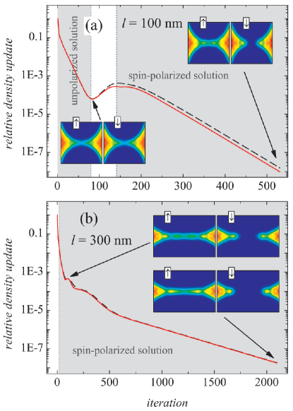
Figure 4: (color online) Convergence of self-consistent calculations for (a) a short QPC ($l=100$ nm) and (b) a long QPC ($l=300$ nm) ($y$-axis corresponds to the relative density update defined by Eq. (9)). Solid and dashed lines denote spin-up and spin-down solutions, respectively. Insets show the charge densities at the constriction at different stages of iteration procedure. Note, that we used the convergence criteria for the relative density update $<10^{-7}$ for all calculations presented in this paper. The geometrical width of the constriction $w=100$ nm; $V_{g}=-1.4$ V.

We now want to focus on an aspects of the calculations concerning a choice of the criteria for termination of the iteration procedure, Eq. (9). Even though this aspect has a rather technical character, we feel that it is important to address it in detail, as the proper choice of the termination criteria is essential for reaching of the spin polarized solution. Figure 4 shows a relative density update as a function of the number of iterations for a relatively short ($l=100$ nm) and a relatively long ($l=300$ nm) constrictions. For the long constriction the spin polarized solution is obtained already during initial iteration steps and its character does not change with increase of the number of iterations, see Fig. 4 (b). On the contrary, for a short constriction, the spin polarized solution is obtained only during later stages of iterations, as no spin-polarized solution is present during the initial steps even when the relative density update decreases to $\sim 10^{-4},$ see 4 (a). Note, that the spin-polarized solution is energetically favorable and more stable than the spin-unpolarized one for all QPC studied.

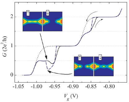
Figure 5: (color online) Conductance hysteresis in the quantum point contact for forward- and backward sweeps of the gate voltage (solid and dashed lines respectively). The dotted line corresponds to the unpolarized solution exhibiting no hysteresis behavior. Insets show the charge densities in the constriction at $V_{g}=-0.975$ V. The parameters of QPC are $l=200$ nm and $w=100$ nm.

The spin-DFT calculations reported above show the presence of the spin-resolved quasi-bound states confined in an effective double-barrier potential. It is well known that the quasi-bound states often lead to the hysteretic behavior of the system. For example, the hysteresis is commonly observed in the I-V characteristics of the resonant double-barrier tunnelling structures for forward- and backward voltage sweepsGoldman ; RTD-book . Such hysteretic behavior is related to the presence of the quasi-bound state between the barriers and was reproduced in numerous calculationsRTD-book , including those based on the DFT approachRTDbistable . Our calculations demonstrate that similar hysteretic behavior is present in the conductance of the QPC. When the gate voltage is swept forward and backwards, the conductance shows the prominent hysteresis in the transition regions between the plateaus, see Fig. 5. In the region of hysteresis, the system, depending on the history, can be in one of two different ground states as illustrated in the inset to Fig. 5. Because the hysteresis is present only in the transition regions and is completely absent in the spin-unpolarized solution, its origin is due to the exchange interaction. We would like to stress that existence of two distinct ground states as well as the hysteresis behavior of the system at hand does not contradict to the DFT approach as such. Owing to the nonlinearity of the problem, there might be more than one solution within the DFT frameworkAlmbladh . Besides the double-barrier resonant tunnelling structures mentioned aboveRTDbistable , the DFT approach was used for the description of the hysteretic behavior of quantum Hall states in the double-layered quantum well structuresMacDonald , as well as hysteresis and spin phase transitions in quantum wires in the integer quantum Hall regimehysteresis . We however, conclude this section by noticing that we are not aware of any experimental reports on the observation of the hysteresis phenomena in the QPC structures.

V Discussion

We start our discussion from a comparison of the spin DFT-based conductance calculations reported in the preceding section with the experimental conductance of the QPC structures. The calculations show a pronounced plateau-like feature at $\sim 0.5\times 2e^{2}/h$ for all QPC structures studied (both short and long ones). For longer QPCs ($l\gtrsim 150$ nm), a dip following 0.5-plateau starts to develop in the conductance. At the same time, a new conductance plateau at $\sim 1.5\times 2e^{2}/h$ starts to develop and a conductance dip following 1.5-plateau also starts to emerge as the length of the constriction increases (see Fig. 2). Our calculations also show a pronounced hysteretic behavior in the transition regions between the plateaus for forward and backward sweeps of the gate voltage, Fig. 5. On the contrary, the experimental data clearly show an anomaly in the conductance around $0.7\times 2e^{2}/h.$ [It should be stressed that the calculated 0.5 plateau corresponds to the complete suppression of one spin channel, whereas experimentally observed 0.7 anomaly means that both spin channels have to be present in the conductance]. Some experimentsReilly_2005 also indicate a feature around $1.7\times 2e^{2}/h$. As far as the hysteresis behavior is concerned, we are not aware of any experimental reports of this effect. The above comparison demonstrates that while the spin-DFT based “first-principle” calculations predict the spin polarization in the QPC structure, the calculated conductance clearly does not reproduce the 0.7 anomaly observed in almost all QPCs of various geometries.

In order to understand why the calculated conductance fails to reproduce the 0.7 anomaly, let us critically analyze the major features of the DFT-based conductance calculations. Our computation scheme relies on an approach that during recent years became a standard tool for transport calculations in open electronic systems such as molecules, metallic wires and mesoscopic conductorsLang ; Guo_open_dot ; Guo ; Ratner ; Datta ; Brandbyge . Its starting point is the Landauer-type formula where the conductance is calculated using the Green’s function or similar scattering techniques combined with the mean-field description of the electronic structure in the leads and in the device region typically based on the ground state self-consistent Kohn-Sham orbitals. Because of the conceptual appeal of this approach, the earlier works were not focused on its formal justification. Recently, however, several studies have provided the rigorous theoretical foundation for the above DFT-based methodologies calculating the steady currents in open electronic systemsAlmbladh ; Evers ; Chen ; Ferretti . Therefore, the question concerning the validity of the present approach relies mostly on the proper description of the exchange and correlation within the DFT approximation. We focus below only on two aspects of the DFT approach that seem to be the most important for understanding of the discrepancy between the calculations and the experiment.

The exchange and correlations are commonly accounted for within the local spin density appromaximationGiuliani_Vignale . As mentioned in preceding sections, for two dimensional systems there are two commonly used parameterizations, namely the parameterization of Tanatar and CeperleyTC and Attacalite et alAMGB . The validity of these approximations was tested for few-electron quantum dot systems and, generally, a very good agreement agreement with the exact diagonalization and/or variational Monte Carlo calculations is foundvalidity . Taking into account that these parametrizations give practically the same results for the QPC conductance, we do not expect the utilization of the above parametrizations to be a source of a significant discrepancy between the calculated conductance and the experiment. Instead, we focus on another aspect of the choice of the exchange energy functional which arises in the systems with a variable particle number. (Note that the QPC structure, being an essentially open structure, belongs to this class of systems). This aspect is related to the infamous “derivative discontinuity problem” of the DFT originating from the discontinuous dependence of $V_{xc}$ on the particle numberGiuliani_Vignale . (Note that the LDA does not include any derivative discontinuity in the $V_{xc}$).

The problem with the derivative discontinuity (leading to uncompensated self-interaction corrections in the $V_{xc}$) has been recently recognized in the standard quantum mechanical transport calculations in molecular systems and atomic wiresEvers ; Toher ; Koentopp . Typically, such the calculations provide a good quantitative agreement with the experimental data for systems where the coupling to the leads is strong and the conductance exceeds the conductance unit $G_{0}=2e^{2}/h$ (for example, for atomistic metallic wires and related systems). At the same time, for weakly coupled systems such as organic molecules the standard DFT+LDA approach leads to the orders-of-magnitude discrepancy between the measured and calculated currents and to incorrect predictions of the conducting (instead of experimentally observed insulated) phaseEvers ; Toher ; Koentopp ; Palacios ; Muralidharan . There have been attempts to explain these discrepancies by insufficient modelling, such as atomistic structures or contact coupling. Several recent studies however, attributed this discrepancy to more fundamental reasons, identifying the lack of the derivative discontinuity in LDA as a major source of error in the DFT-based transport calculationsToher ; Koentopp . For example, Toher et al.Toher argue that LDA approximation is not suitable for transport calculations for the case of weak coupling. They propose a simple corrective scheme based on the removal of the atomic self-interaction. Their corrective scheme restores an agrement with the experiment, opening a conduction gap of the I-V characteristics of a molecular junction instead of a metallic behavior following from the standard DFT+LDA approach. (It is interesting to note that similar self-interaction corrections practically do not effect the conductance and electronic density for the case of strongly-coupled systemsToher ). Alternative corrective schemes replacing the Kohn-Sham data for the weakly coupled region with their counterparts obtained from a Hartree-Fock analysis (taking care of the self-interaction problem) are suggested by Evers et al.Evers and PalaciosPalacios . Note that various approaches to the description of quantum transport for the case of weakly coupled systems (accounting for the charge quantization and thus eliminating the self-interaction errors) were discussed in Refs. Indlekofer, ; Wacker, ; Muralidharan, .

We argue here that a similar problem related to the derivative discontinuity may be the reason why the standard DFT+LDA approach fail to describe the observed 0.7-anomaly in the QPC. Indeed, the formation of a spin-polarized charge droplet predicted within the DFT+LDA approach implies that electrons are trapped in weakly coupled quasi-bound states in the center of the QPC. As mentioned above, in the case of weak coupling the lack of the derivative discontinuity in the LDA approximation causes the orders-of-magnitude discrepancies between the theory and experiment for the molecular systems. Thus, it would be reasonable to expect that due to the same reason the LDA approximation is not suitable for the case of the QPC structure as well. Because the corrective schemes accounting for the derivative discontinuity are shown to strongly affect the electron density and the energy levels in the system, and because of the apparent failure of the standard DFT+LDA approach to reproduce the 0.7 anomaly, we conclude that the formation of the magnetic impurities in the QPC might be an artefact of the LDA due to the lack of the derivative discontinuity related to the spurious self-interaction.

Based on the above discussion we conclude that an accurate description of the QPC structure might require approaches that go beyond the standard DFT+LDA scheme and account for the derivative discontinuity in the $V_{xc}$ or utilize similar corrective schemes eliminating the self-interaction errors of the DFT+LDA. It is not clear at the moment whether the recipes for the accounting of the derivative discontinuity and eliminating the self-interaction correction developed for the molecular junctionsToher ; Evers ; Palacios can be adapted for the QPC structure. Such the corrective schemes are remained to be implemented and it remains to be seen whether this can bring the calculated conductance to the closer agreement with the experiment.

As an indirect support of the above arguments we notice that similar spin DFT conductance calculations (within the same LDA approach and the same parameterization of $V_{xc}$)Marcus_paper reproduce quantitatively the measured spin-resolved magnetoconductance of the QPCs in the integer quantum Hall regimeRadu . In this case the edge state regime is reached such that the transport through the QPC correspond to the strong coupling regime.

Finally, a comment is in order concerning the Kondo physics. The Kondo effect was suggested by Cronenwett et al.Cronenwett as a possible source of the 0.7 anomaly; at the same time, the experimental studies of GrahamGraham RokhinsonRokhinson seem to rule out this interpretation. We stress that the present mean-field approach based on the standard DFT+LDA formulation is not able to address this effect. Moreover, we do not believe that the prediction of the magnetic impurity formation within the DFT+LDA approach can support or rule out the Kondo physics in the QPC. Indeed, the Kondo enhanced conductance channels (if they exist) would change the electron density inside the QPC (beyond that one predicted by the DFT). Thus, the DFT+LDA predictions for the equilibrium electron density in the QPC should be corrected in a self-consistent way to account for this additional density, and it is not obvious whether the spin-polarized quasi-bound states predicted in the framework of the DFT+LDA would survive this correction.

VI Conclusion

We have developed an approach for full quantum mechanical transport conductance calculations in open lateral split-gate structures that starts from the lithographical layout of the device and is free from phenomenological parameters like coupling strengths, charging constants etc. The whole structure, including the semi-infinitive leads, is treated on the same footing (i.e. the electron-electron interaction is accounted for in both the leads as well as in the central device region). The electron-electron interaction and spin effects are included within the spin density functional theory in the local spin density approximation, and the conductance calculated on the basis of the standard Green’s function technique.

The developed method was applied to calculate the spin-resolved conductance through a QPC. Close to the pinch off a spin-degeneracy of the spin-up and spin-down conductance channels is lifted and the total conductance shows a broad feature peaked at $0.5\times 2e^{2}/h$ (corresponding to a complete suppression of one of the spin channels). A similar feature is also present in the range of the gate voltages where a second step in the conductance develops. The lifting of the spin-degeneracy and the suppression of one of the spin channels are the generic features of all studied QPCs (both very short and very long; $40\lesssim l\lesssim 500$ nm). The calculated conductance also shows a hysteresis for forward- and backward sweeps of the magnetic fields. These features in the conductance are related to the formation of weakly coupled (quasi-bound) states in the constriction of the QPC (predicted in previous DFT-based studiesMeir_2003 ; Meir_Nature ). A comparison of the obtained results with the experimental data shows however, that while the spin-DFT based “first-principle” calculations predict the spin polarization in the QPC structure, the calculated conductance clearly does not reproduce the 0.7 anomaly observed in almost all QPCs of various geometries.

In order to understand why the calculated conductance fails to reproduce the 0.7 anomaly, we critically examine the major features of the DFT-based conductance calculations. We suggest that inability of the standard DFT+LDA approximation to reproduce the 0.7 anomaly might be related to infamous derivative discontinuity problem of the DFT leading to spurious self-interaction errors not corrected in the standard LDAGiuliani_Vignale . This problem has been recently recognized in similar DFT-based transport calculations for the molecular junctions (showing orders-of-magnitude discrepancies with the experiment) where it has been demonstrated that the LDA approximation is not suitable for transport calculations for the case of weak couplingToher ; Koentopp . We thus conclude that the formation of the weakly coupled magnetic impurities in the QPC might be an artefact of the LDA due to the lack of the derivative discontinuity and related spurious self-interaction. Our results suggest that an accurate description of the QPC structure requires approaches that go beyond the standard DFT+LDA scheme and that account for the derivative discontinuity in the $V_{xc}$ or utilize similar corrective schemes eliminating the self-interaction errors of the DFT+LDA.

- (1) K. J. Thomas, J. T. Nicholls, M. Y. Simmons, M. Pepper, D. R. Mace, and D. A. Ritchie, Phys. Rev. Lett. 77, 135 (1996).
- (2) K. J. Thomas, J. T. Nicholls, N. Y. Appleyard, M. Y. Simmons, M. Pepper, D. R. Mace, W. R. Tribe, and D. A. Ritchie, Phys. Rev. B 58, 4846 (1996).
- (3) A. Kristensen, P. E. Lindelof, J. B. Jensen, M. Zaffalon, J. Hollingbery, S. W. Pedersen, J, Nygard, H. Bruus, S. M. Reimann, S. B. Sorensen, M. Michel, and A. Forchel, Physica B 251, 180 (1998).
- (4) B. E. Kane, G. R. Facer, A. S. Dzurac, N. E. Lumpkin, R. G. Clark, L. N. Pfeiffer, and K. W. West, Appl. Phys. Lett. 72, 3506 (1998).
- (5) D. J. Reilly, G. R. Facer, A. S. Dzurak, B. E. Kane, R. G. Clark, P. J. Stiles, R. G. Clark, A. R. Hamilton, J. L. O’Brien, N. E. Lumpkin, L. N. Pfeiffer, and K. W. West, Phys. Rev. B 63, 121311(R), (2001).
- (6) S. M. Cronenwett, H. J. Lynch, D. Goldhaber-Gordon, L. P. Kouwenhoven, C. M. Markus, K. Hirose, N. S. Wingreen, and V. Umansky, Phys. Rev. Lett. 88, 226805 (2002).
- (7) D. J. Reilly, T. M. Buehler, J. L. O’Brien, A. R. Hamilton, A. S. Dzurak, R. G. Clark, B. E. Kane, L. N. Pfeiffer, and K. W. West, Phys. Rev. Lett. 89, 246801 (2002).
- (8) D. J. Reilly, Phys. Rev. B 72, 033309 (2005).
- (9) A. C. Graham, M. Pepper, M. Y. Simmons, and D. A. Ritchie, Phys. Rev. B 72, 193305 (2005).
- (10) L. P. Rokhinson, L. N. Pfeiffer, and K. W. West, Phys. Rev. Lett. 96, 156602 (2006).
- (11) K.-F. Berggren and I. I. Yakimenko, Phys. Rev. B 66, 085323 (2002).
- (12) A. A. Starikov, I. I. Yakimenko, and K.-F. Berggren, Phys. Rev. B 67, 235319 (2003).
- (13) P. Jaksch, I. I. Yakimenko, and K.-F. Berggren, Phys. Rev. B 74, 235320 (2006).
- (14) P. Havu, M. J. Puska, R. M. Nieminen, and V. Havu, Phys. Rev B 70, 233308 (2004).
- (15) Y. Meir, K. Hirose, and N. S. Wingreen, Phys. Rev. Lett. 89, 196802 (2002).
- (16) K. Hirose, Y. Meir, and N. S. Wingreen, Phys. Rev. Lett. 90, 026804 (2003).
- (17) T. Rejec and Y. Meir, Nature 442, 900 (2006).
- (18) I. A. Shelykh, N. G. Galkin, and N. T. Bagraev, Phys. Rev. B 74, 085322 (2006).
- (19) D. A. Wharam, T. J. Thornton, R. Newbury, M. Pepper, H. Ahmed, J. E. F. Frost, D. G. Hasko, D. C. Peacock, D. A. Ritchie, and G. A. C. Jones, J. Phys. C 21, L209 (1988); B. J. van Wees, H. van Houten, C. W. J. Beenakker, J. G. Williamson, L. P. Kouwenhoven, D. van der Marel, and C. T. Foxon, Phys. Rev. Lett. 60, 848 (1988).
- (20) H. Bruus, V. V. Cheianov, and K. Flensberg, Physica E (Amsterdam) 10, 97 (2001).
- (21) J. H. Davies, I. A. Larkin, and E. V. Sukhorukov, J. Appl. Phys. 77, 4504 (1995).
- (22) J. Martorell, H. Wu, and D. W. L. Sprung, Phys. Rev. B 50, 17298 (1994).
- (23) G. F. Giuliani and G. Vignale, Quantum Theory of the Electron Liquid, (Cambridge University Press, Cambridge, 2005).
- (24) B. Tanatar and D. M. Ceperley, Phys. Rev. B 39, 5005, (1989).
- (25) C. Attacalite, S. Moroni, P. Gori-Giogri, and G. B. Bachelet, Phys. Rev. Lett. 88, 256601 (2002); P. Gori-Giorgi, C. Attacalite, S. Moroni, and G. B. Bachelet, Int. J. Quantum Chem. 91, 126 (2003).
- (26) S. Datta, Electronic Transport in Mesoscopic Systems, (Cambridge University Press, Cambridge, 1997).
- (27) S. Ihnatsenka, I. V. Zozoulenko, and M. Willander, cond-mat/0701107.
- (28) S. Ihnatsenka and I. V. Zozoulenko, Phys. Rev. B 73, 075331 (2006).
- (29) I. V. Zozoulenko, F. A. Maaø and E. H. Hauge, Phys. Rev. 53, 7975 (1996); Phys. Rev. 53, 7987 (1996); Phys. Rev. 56, 4710 (1997).
- (30) D. Singh, H. Krakauer, and C. S. Wang, Phys. Rev. B 34, 8391 (1986).
- (31) V. J. Goldman, D. C. Tsui, and J. E. Cunningham, Phys. Rev. Lett. 58, 1256 (1987).
- (32) H. Mizuta and T. Tanouesee, The Physics and Applications of Resonant Tunnelling Diodes, (Cambridge University Press, Cambridge, 1997).
- (33) N. Zou, M. Willander, I. Linnerud, U. Hanke, K. A. Chao, and Y. M. Galperin, Phys. Rev. B 49, 2193 (1994); G. Klimeck, R. Lake, and D. K. Blanks, Phys. Rev. B 58, 7279 (1998).
- (34) G. Stefanucci and C.-O. Almbladh, Phys. Rev. B 69, 195318 (2004).
- (35) V. Piazza, V. Pellegrini, F. Beltram, W. Wegscheider, T. Jungwirth, and A. H. MacDonald, Nature 402, 638 (1999).
- (36) S. Ihnatsenka and I. V. Zozoulenko, Phys. Rev. B 75, 035318 (2007).
- (37) N. D. Lang, Phys. Rev. B 52, 5335 (1995); N. D. Lang and Ph. Avouris, Phys. Rev. Lett. 81, 3515 (1998)
- (38) Y. Wang, J. Wang, H. Guo, and E. Zaremba, Phys. Rev. B 52, 2738 (1995).
- (39) J. Taylor, H. Guo, and J. Wang, Phys. Rev. B 63, 245407 (2001).
- (40) Y. Xue, S. Datta and M. A. Ratner, J. Chem. Phys. 115, 4292 (2001)
- (41) P. S. Damle, A. W. Ghosh, and S. Datta, Phys. Rev. B 64, 201403(2001).
- (42) M. Brandbyge, J.-L. Mozos, P. Ordejon, J. Taylor, and K. Stokbro, Phys. Rev. B 65, 165401 (2002).
- (43) F. Evers, F. Weigend, and M. Koentopp, Phys. Rev. B 69, 235411 (2004).
- (44) X. Zheng and G. H. Chen, physics/0502021.
- (45) A. Ferretti, A. Calzolari, R. Di Felice, and F. Manghi, Phys. Rev. B 72, 125114 (2005).
- (46) H. Saarikoski, E. Räasäanen, S. Siljamäaki, A. Harju, M. J. Puska, and R. M. Nieminen, Phys. Rev. B 67, 205327 (2003); E. Räsänen, H. Saarikoski, V. N. Stavrou, A. Harju, M. J. Puska, and R. M. Nieminen, Phys. Rev B 67, 235307 (2003); M. Borgh, M. Toreblad, M. Koskinen, M. Manninen, S. Åberg, and S. M. Reimann, Intl. J. Quant. Chem. 105, 817 (2005).
- (47) C. Toher, A. Filippetti, S. Sanvito, and K. Burke, Phys. Rev. Lett. 95, 146402 (2005).
- (48) M. Koentopp, K. Burke, F. Evers, Phys. Rev. B 73, 121403(R) (2006).
- (49) J. J. Palacios, Phys. Rev. B 72, 125424 (2005).
- (50) B. Muralidharan, A. W. Ghosh, and S. Datta, Phys. Rev. B 73, 155410 (2006).
- (51) K. M. Indlekofer, J. Knoch, and J. Appenzeller, Phys. Rev. B 72, 125308 (2005).
- (52) J. N. Pedersen and A. Wacker, Phys. Rev. B 72, 195330 (2005).
- (53) S. Ihnatsenka and I. V. Zozoulenko, to be published.
- (54) I. P. Radu, J. B. Miller, S. Amasha, E. Levenson-Falk, D. M. Zumbuhl, M. A. Kastner, C. M. Marcus, L. N. Pfeiffer, and K. W. West, to be published.