Evolution of entanglement after a local quench

Abstract

We study free electrons on an infinite half-filled chain, starting in the ground state with a bond defect. We find a logarithmic increase of the entanglement entropy after the defect is removed, followed by a slow relaxation towards the value of the homogeneous chain. The coefficients depend continuously on the defect strength.

and

1 Introduction

The entanglement properties of quantum chains in their ground state are by now rather well known. The most common measure is the entanglement entropy calculated with the reduced density matrix for a subsystem, usually a segment of the chain. This quantity was first studied within field theory [1] and more recently also for various lattice models [2, 3, 4, 5, 6, 7]. For non-critical systems it is finite and of order one, but for critical systems it diverges logarithmically with the length of the subsystem. Moreover, the prefactor of the logarithm is given by the central charge $c$ in the conformal classification, see [5]. In systems with defects or disorder it may be modified [8, 9, 10].

A more complex situation arises if the quantum state evolves in time. The simplest way to achieve this is a quench, where one changes a parameter of the system instantaneously. An eigenstate of the initial Hamiltonian then becomes a superposition of the eigenstates of the final one and a complicated dynamics results. The concomitant evolution of the entanglement entropy has been the topic of several recent studies [11, 12, 13, 14]. If one is dealing with critical models, this can be discussed within conformal field theory [11].

So far, most quenches considered were global, i.e. the system was modified everywhere in the same way. Such a quench can actually be realized for atoms in optical lattices [15]. In the theoretical studies, it was found that the entanglement entropy first increases linearly in time and then saturates at a value proportional to the size of the subsystem. Thus it becomes an extensive quantity, in contrast to the equilibrium case. These features can be understood in a simple picture where pairs of particles transmit the entanglement from the initial state to later times [11, 12].

In the present paper we study a different situation, namely a local quench. We consider free electrons hopping on a chain which initially contains a defect in form of a weakened bond. This defect is suddenly removed and the electronic system has to readjust. The set-up is similar to the X-ray absorption problem in metals where the creation of a deep hole leads to a local scattering potential. When a conduction electron fills the hole, this potential is switched off again [16].

In contrast to a related study of the transverse Ising model [17], we start from the ground state. We consider a section of the chain containing the defect in the interior or at its boundary and calculate the time evolution of its entanglement entropy with the rest. For the equilibrium case, this problem has been studied before [8]. We find a time dependence which is very different from that for a global quench. The entanglement entropy only changes after a certain waiting time, increases then to a maximum or plateau, depending on the location of the defect, and finally decreases very slowly and in a universal way towards its equilibrium value. In particular, it remains always non-extensive.

The calculations are numerical and based on the determination of the reduced density matrix $\rho$ from the one-particle correlation functions. The necessary formulae are given in section 2. The case of a central defect, typical single-particle eigenvalue spectra and the long-time behaviour of S are discussed in section 3. The evolution of the entropy at intermediate times and for various defect positions is presented in section 4. The case of a boundary defect is studied in section 5 and described by simple formulae based on fronts moving through the system. In section 6 we sum up our findings. In the two appendices we discuss the initial entanglement and present a simple example of a global quench for comparison.

2 Model

We consider a system of free spinless fermions hopping between neighbouring sites of an infinite chain (XX model). The system is half filled and initially prepared in the ground state of the inhomogeneous Hamiltonian

$$H_{0}=-\frac{1}{2}\sum_{n=-\infty}^{\infty}t_{n}(c_{n}^{\dagger}c_{n+1}+c_{n+1}^{\dagger}c_{n})\,,$$ (1)

where the hopping amplitudes are $t_{0}=t^{\prime}$ and $t_{n}=1$ for $n\neq 0$. Thus one has a single bond defect between sites $0$ and $1$. At time $t=0$ this defect is removed and the time evolution is governed by the homogeneous Hamiltonian

$$H_{1}=-\frac{1}{2}\sum_{n=-\infty}^{\infty}(c_{n}^{\dagger}c_{n+1}+c_{n+1}^{\dagger}c_{n})\,.$$ (2)

Both $H_{0}$ and $H_{1}$ describe critical systems. Our aim is to study how the entanglement between a subsystem of length $L$ and the rest of the chain evolves after the quench. The subsystem is chosen in such a way that the initial defect is inside of it or at its boundary.

The entanglement properties are determined by the reduced density matrix which for free fermions has the following diagonal form [18, 19]:

$$\rho_{L}=\frac{1}{\tilde{Z}}e^{-\tilde{H}}\;,\quad\tilde{H}=\sum_{k=1}^{L}\varepsilon_{k}(t)f_{k}^{\dagger}f_{k}\,.$$ (3)

Here $\tilde{Z}$ is a normalization constant ensuring $\mathrm{tr}\,\rho_{L}=1$ and the fermionic operators $f_{k}$ follow from the $c_{n}$ by an orthogonal transformation. The eigenvalues $\varepsilon_{k}(t)$ are given by

$$\varepsilon_{k}(t)=\ln\frac{1-\zeta_{k}(t)}{\zeta_{k}(t)},$$ (4)

where $\zeta_{k}(t)$ are the eigenvalues of the time-dependent ($L\times L$) correlation matrix

$$C_{jl}(t)=\langle 0|\,c_{j}^{\dagger}(t)\,c_{l}(t)\,|0\rangle\,.$$ (5)

Here $|0\rangle$ is the ground state of $H_{0}$ and the indices $j$ and $l$ run over the sites of the subsystem. The $\zeta_{k}(t)$ also determine the entanglement entropy $S=-\mathrm{tr}(\rho_{L}\ln\rho_{L})$ via

$$S(t)=-\sum_{k}\zeta_{k}(t)\ln\zeta_{k}(t)-\sum_{k}(1-\zeta_{k}(t))\ln(1-\zeta_{k}(t))\,.$$ (6)

To obtain the matrix ${\bf{C}}(t)$ one diagonalizes the operator $H_{1}$ by a Fourier transform

$$H_{1}=-\sum_{q}\cos q\;c^{\dagger}_{q}c_{q}\,.$$ (7)

The time dependence of the $c_{q}$ then is $c_{q}(t)=\exp(it\cos q)\,c_{q}$ and Fourier transforming back gives, for a ring of $N$ sites,

$$c_{j}(t)=\sum_{m}U_{jm}(t)c_{m}\,,\quad U_{jm}(t)=\frac{1}{N}\sum_{q}\mathrm{e}^{-iq(j-m)}\mathrm{e}^{it\cos q}\,.$$ (8)

In the thermodynamic limit, the matrix elements $U_{jm}(t)$ of the unitary evolution operator can be written as Bessel functions and the correlation matrix becomes

$$C_{jl}(t)=i^{l-j}\sum_{m,n}i^{m-n}J_{j-m}(t)J_{l-n}(t)C_{mn}(0)\,.$$ (9)

This expresses ${\bf{C}}(t)$ in terms of the matrix ${\bf{C}}(0)$ calculated with the initial state $|0\rangle$. The information is transmitted via the Bessel functions which have a maximum when the spatial separation is equal to the elapsed time. The factors in front of the Bessel functions can lead to imaginary correlations and thus to local currents in the system. This is what one also expects on physical grounds.

The initial matrix elements $C_{mn}(0)$ were already obtained in [8] for the region to the right of the defect. Then they have the form

$$C_{mn}(0)=C^{0}_{mn}-C^{1}_{mn}\,,\quad m,n>0$$ (10)

where $C^{0}_{mn}$ denotes the correlation matrix of the homogeneous system

$$C^{0}_{mn}=\frac{\sin\left[\frac{\pi}{2}(m-n)\right]}{\pi(m-n)}$$ (11)

and $C^{1}_{mn}$ is the contribution of the defect, given explicitly in Eq. (8) of [8]. It depends only on $m+n$ and vanishes for $t^{\prime}=1$. If the defect cuts the chain, $C^{1}$ reduces to $C^{0}$ with argument $m+n$. When both sites are to the left of the defect, one simply has to replace $m+n$ with $m+n-2$, and by a straightforward generalization one can obtain corresponding formulae for $m$ and $n$ on opposite sides of the defect.

With these initial values, the correlation matrix ${\bf{C}}(t)$ was calculated numerically and then diagonalized to obtain the eigenvalue spectrum and the entanglement entropy. Since the Bessel functions decay rapidly for indices much larger than the argument $t$, one can confine each of the sums in (9) to about $(2t+4L)$ terms. Most calculations were done for times of the order 100-200.

3 Central defect and spectra

We start with analyzing a simple symmetric situation, namely a defect with $t^{\prime}=0$ in the center of the subsystem. Thus one starts with two uncoupled infinite half-chains which then are connected.

In Figure 1 the time evolution of the single-particle spectrum is shown in two different ways. On the left hand side, the eight lowest eigenvalues $\varepsilon_{k}(t)$ are plotted in ascending order for several times. Only the positive ones are shown, since due to the half-filling the spectrum is symmetric with respect to zero. These snapshots show that the initial step structure resulting from the degeneracies of the uncoupled chains smoothens with time and the dispersion curve seems to approach the one of the homogeneous system. However, two steps remain and as a consequence the curves lie below the asymptotic one. Roughly speaking, this corresponds to a stronger entanglement.

Figure 1: Time evolution of the low-lying single-particle eigenvalues $\varepsilon_{k}(t)$ for a subsystem of $L=40$ sites with a central defect $t^{\prime}=0$. Left: snapshots of the positive eigenvalues for different times, compared with the spectrum in equilibrium. Right: time evolution of the four lowest eigenvalues.

On the right, the time evolution of the four lowest eigenvalues is displayed. It shows two important features. Firstly, the eigenvalues remain unchanged and the two-fold degeneracy survives up to a time $T\approx L/2$. This can be explained in terms of a front propagating with velocity $v=1$ [20] which is the Fermi velocity in the system and also the speed of the maxima in the Bessel functions. Before the front, starting at the defect, reaches the boundary, the subsystem to the right (left) of the defect cannot become entangled with the environment to the left (right).

Secondly, for $t>T$ three of the eigenvalues quickly relax towards the values $\varepsilon_{k}^{h}$ of the homogeneous system but one, on the contrary, starts to evolve rather slowly. These “anomalous” eigenvalues (another one is found among the higher levels) lead to the kinks in the dispersion curves on the left of Fig. 1 when they are close to another level. The smallest one is the most important for the entanglement, and its time dependence will determine that of $S$, since the other $\varepsilon_{k}(t)$ are basically constant.

Therefore it is important to have a general picture of its behaviour. Figure 2 shows what happens for times $t$ up to 1600. In contrast to Figure 1, where the anomalous eigenvalue simply crossed over, one sees an avoided crossing with the next one, $\varepsilon_{5}$, which already looked relaxed at smaller times. This can be attributed to the fact that the two eigenstates in this case have the same reflection symmetry.

Figure 2: Large-time behaviour of the eigenvalues $\varepsilon_{4}(t)$ and $\varepsilon_{5}(t)$ already seen in Figure 1. The avoided level crossing can be fitted by $\ln(t/\tau)$ with $\tau\approx 1$.

At the avoided crossing, the two eigenvalues exchange role and the anomalous parts of the curves can be well described by a single logarithm of the form $\ln(t/\tau)$, as shown in the Figure. Therefore the spectrum roughly looks as in equilibrium with at least one additional eigenvalue $\varepsilon_{an}$. One expects that for very large times $\varepsilon_{an}$ finally converges to the maximal eigenvalue of the homogeneous system. Therefore the logarithmic behaviour cannot persist indefinitely. This could be confirmed for a rather small subsystem with $L=6$ sites, but for larger $L$ the necessary times are numerically inaccessible. Moreover, the $\varepsilon_{k}$ can only be calculated reliably for values up to about 25.

One can also look at the single-particle eigenfunctions connected with the $\varepsilon_{k}$. Then one finds that they develop imaginary parts which vanish again as the eigenvalue approaches the equilibrium limit. In the anomalous eigenvector they persist more and generally speaking this eigenvector looks more extended than the others when $\varepsilon_{an}$ is not close to a crossing.

The entanglement entropy, finally, is shown in Figure 3. The basic features are consequences of eigenvalue spectrum discussed above. One has a sudden jump at $t=T$, followed by a very slow relaxation towards $S_{h}$, the value in the homogeneous system. For a large subsystem, initial and final value of $S$ are also the same, as discussed in Appendix A.

Figure 3: Time evolution of the entanglement entropy for a subsystem of $L=40$ sites with a central defect $t^{\prime}=0$. A sudden jump is followed by a slow relaxation towards the homogeneous value $S_{h}$. The inset shows the logarithmic correction to the $1/t$ decay.

As mentioned above, the slow decay can be understood in terms of the anomalous eigenvalue $\varepsilon_{an}$. Its observed logarithmic time dependence implies $\zeta_{an}(t)\approx\tau/t$. This yields for the entropy

$$S(t)=S_{h}+\frac{\alpha\ln(t)+\beta}{t}.$$ (12)

The inset in Figure 3 shows that the logarithmic corrections to the $1/t$ time dependence can be indeed observed and fitted very well.

The height of the maximum in $S$ depends on the size of the subsystem and one finds the behaviour

$$S_{m}-S_{h}=\frac{c_{m}}{3}\ln L+k_{m}\,,$$ (13)

where $c_{m}\approx 0.23$ and $k_{m}\approx 0.06$.

All these results were obtained for a defect with $t^{\prime}=0$. However, they also hold for the general case $0<t^{\prime}<1$. Then the spectra and the entropy have similar behaviour only the amplitude $c_{m}$ and the constant $k_{m}$ decrease with increasing $t^{\prime}$, since the effect must vanish for $t^{\prime}=1$.

4 Entropy and defect position

We now ask how the picture changes if one varies the position of the defect. For simplicity we discuss the case $t^{\prime}=0$, in which the defect cuts the subsystem into two parts with $L_{1}$ sites to the left and $L_{2}=L-L_{1}$ to the right of it.

Figure 4 shows the entropy for intermediate times and several defect positions, specified by the numbers $L_{1}$ and $L_{2}$. The extreme cases are a defect at the boundary, $L_{1}=0$, and in the center $L_{1}=L/2$, as in the previous section. The main feature is the development of a plateau-like region, which can be understood in terms of fronts propagating from the defect site. The entropy increases rapidly at $T_{1}\approx L_{1}$ when one of the fronts reaches the closest boundary and starts to decay at $T_{2}\approx L_{2}$ when both fronts have left the subsystem. Thus the plateau is related to the asymmetry of the set-up.

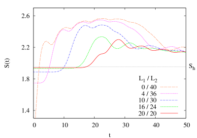
Figure 4: Time evolution of the entropy for a subsystem of $L=40$ sites for several defect positions $L_{1}/L_{2}$, indicating the number of sites to the left/right of the defect with $t^{\prime}=0$.

One also finds that at time $t=L_{2}$ where the plateau region ends, the entropy always has the same value which moreover coincides with the maximum value (13) found for the central defect in the previous section. Beyond this point, the long-time region begins and shows the same relaxation behaviour as in (12) for all defect positions, although the curves do not coincide completely when shifted appropriately. The plateau itself will be studied in more detail in the following section.

5 Defect at the boundary

To obtain a better understanding of the development of the entropy plateau we now investigate the situation when it is most pronounced. This is the case for a defect located at the boundary of the subsystem. The behaviour for these intermediate times should be connected with the propagation of a wavefront in the subsystem. That such a front actually exists, can be seen from the single-particle eigenfunctions.

In Figure 5 we show snapshots of the lowest eigenvector for several intermediate times in a subsystem of $L=100$ sites. One can clearly recognize the front, either from the real part or from the imaginary part of the eigenvector. The latter, in particular, only develops behind the front, while it is approximately zero otherwise.

Figure 5: Snapshots from the time evolution of the eigenvector corresponding to the lowest lying single-particle eigenvalue of a subsystem with $L=100$ sites and with a defect $t^{\prime}=0$ at the left boundary.

Furthermore, the form of the eigenvectors suggests to interpret the front as an effective defect with a time-dependent position, which divides the subsystem in two parts of size $t$ and $L-t$. This leads to an analogy with the equilibrium problem where the defect is located inside a subsystem. Some details for this situation, which was not covered in [8] are given in Appendix A. In that case, the entropy can be written as a sum of logarithmic terms, which can be combined into a scaling function depending only on $x/L$ and $1-x/L$ where $x$ is the location of the defect.

Starting from these equilibrium formulae, one is lead to make the following generalized ansatz for the nonequilibrium case

$$f(t,L)=\frac{c_{1}}{3}\ln(1+t)+\frac{c_{2}}{3}\ln(1+L-t)+k,$$ (14)

where each of the coefficients depends on the strength of the defect. Note, that one has to have $c_{1}\neq c_{2}$ in order to account for the nonsymmetric plateaus. The arguments of the logarithms have been shifted to avoid divergences in the interval $\left[0,L\right]$.

In the simplest case of zero defect strength one can also motivate the ansatz (14) with the help of a simple physical picture. Initially one has a subsystem which is entangled only with one of the half-chains and corresponding entropy $S\sim 1/6\,\ln L$. The propagating front carries information about the other half-chain, and therefore the $t$ sites of the subsystem which have already been visited by the front acquire an entropy $S\sim 1/3\,\ln t$, while the other $L-t$ sites still remain entangled only with one half-chain. This gives the values $c_{1}=1$ and $c_{2}=1/2$ for the constants.

Figure 6 shows the entropy plateau curves with $t^{\prime}=0$ for different system sizes, together with the fit functions (14). Our fit gave the values $c_{1}=0.96$, $c_{2}=0.55$ and $k=1.03$. We emphasize, that these coefficients have been obtained via a single fit to the $L=200$ data, and the other two curves differ only in the parameter $L$. One can see a good agreement with the data, except for the boundaries of the time intervals. Indeed, for $t=L$ the fit formula (14) scales as $S\approx 1/3\,\ln L$, that is the asymptotics of the equilibrium entropy $S_{h}$. However, as it was mentioned in the previous section, the value $S(t=L)$ is described by (13), and for later times one enters in the regime of slow relaxation towards $S_{h}$.

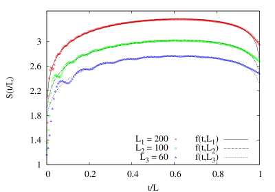
Figure 6: Entropy plateaus in case of a $t^{\prime}=0$ boundary defect for different subsystem sizes. The fitting function is defined in Eq. (14) and the coefficients were determined by a single fit to the $L=200$ data.

The situation becomes slightly more complicated for arbitrary defect strengths in the range $0\leq t^{\prime}\leq 1$. Considering the limiting case $t^{\prime}=1$ one has no time dependence at all, thus $c_{1}=c_{2}=0$, however the entropy in this homogeneous case must scale as $S\sim 1/3\,\ln L$. Therefore the constant in (14) must be rewritten to contain a term proportional to $\ln L$ with a new coefficient. Finally, one could change to the scaling variables $t/L$ and write the entropy in the form

$$S(t,L)=\frac{c_{0}}{3}\ln L+\frac{c_{1}}{3}\ln(t/L)+\frac{c_{2}}{3}\ln(1-t/L)+k^{\prime},$$ (15)

where all the parameters $c_{0},c_{1},c_{2}$ and $k^{\prime}$ are functions of the defect strength and have to be determined by fitting to the data. Note, that the above form of the entropy is expected to hold only for large $L$ and away from the boundaries of the time interval.

In fact, we have always used the regularised ansatz (14) to determine the $t^{\prime}$-dependence of $c_{1},c_{2}$ and $k$ by fitting to time series with $L=100$ fixed. Then the additional logarithmic term was extracted from fitting to the $k$ values obtained from time series with different $L$, $t^{\prime}$ being fixed. One finds after all, that $c_{0}\approx 1+c_{2}$, thus one needs only $c_{1},c_{2}$ and $k^{\prime}$ to describe the plateaus. The $t^{\prime}$-dependence of the former two is depicted in Figure 7. One can see that the coefficients vary smoothly with $t^{\prime}$, both of them going to zero as $t^{\prime}\to 1$.

Figure 7: Scaling function coefficients $c_{1}$ and $c_{2}$ as functions of the defect strength.

In conclusion, the time dependence of the entropy in the plateau-region can be written in the scaling form (15) for all values of the defect strength. The effective height of the plateau scales as $c_{0}/3\,\ln L$ with $c_{0}>1$ which indicates a logarithmic increase of the entropy for these intermediate times.

6 Summary and conclusions

We have studied a particular kind of quench, where the system remained critical and was only modified locally. Starting from the ground state with a defect, we calculated the evolution of the reduced density matrix and the entanglement following from it. The main effect is an increase of the entropy $S$ on a time scale $t\approx L$ which can be related to the excitations near the Fermi energy with velocity $v_{F}=1$ in our units. Thus the entanglement always increases at the early stages of the rearrangement process. The criticality of the system is reflected in the logarithmic dependence of various quantities, in particular the height of the maximum of $S$, on the size of the subsystem. For the case of a boundary defect, where the mechanism at work leads to a plateau, we could also find the scaling function describing its shape. The defect strength only changes the parameters, which are closely related to those in equilibrium, but not the qualitative features. The long-time behaviour is characterized by a slow approach to the homogeneous ground state. For the times accessible, one finds a universal law independent of the defect strength. Thus no anomalous exponents as in the X-ray problem enter. These appear for time-delayed correlation functions or in the overlap between initial and time-dependent state, whereas here one is following the evolving state directly.

A particular feature of our situation is that the initial state is asymptotically degenerate with the final ground state. This distinguishes it from the case of global quenches, where the energy difference between both is extensive, and also from the study in [17], where the evolution started from a randomly chosen high-energy state and the main interest was in the thermalization. On the level of the reduced density matrix, one can define an effective temperature, if $\rho$ has thermal form, which is always the case for free fermions, and if the $\varepsilon_{k}$, or at least the important ones, are proportional to the single-particle excitations of the Hamiltonian. This is the case for critical systems where both have linear dispersion [21] and also for the global quench considered in Appendix B. In this sense, our subsystem thermalizes with an effective temperature $T_{eff}=\ln L/\pi L$ which vanishes if one considers the whole system, while the quench in Appendix B leads to a finite value $T_{eff}=1/2$.

Altogether we have obtained a good overall picture of the phenomena, although some aspects like the oscillations in $S$ and the influence of the filling have not been addressed. However, an analytical derivation of the asymptotic time dependence would still be desirable.

Appendix A: Initial entanglement

For a defect at the boundary of the subsystem, the entanglement entropy has already been studied in [8]. For a general location, an expression can be given immediately if $t^{\prime}=0$. Then one has two half-chains where segments at the ends are part of the subsystem. If their respective lengths $l$ and $L-l$ are large, the conformal formulae [5] lead to

$$S=\frac{c}{6}\bigl{[}\,\ln(l)+\ln(L-l)\,\bigr{]}+2k_{1}$$ (16)

where $c=1$ and $k_{1}\approx 0.479$ for the hopping model. Thus $S$ is maximal when the defect is in the center of the subsystem, $l=L/2$.

Numerical calculations show that this law also holds for arbitrary defect strengths $t^{\prime}\leq 1$ but with a constant $c^{\prime}$ depending on $t^{\prime}$. Measuring the position of the defect from the center of the subsystem, $l=L/2+x$, one can write it in the form

$$S=\bigl{[}\,\frac{1}{3}\ln L+k\,\bigr{]}+\frac{c^{\prime}}{3}\ln\,\bigl{[}\,1-(\frac{2x}{L})^{2}\;\bigr{]},$$ (17)

The term in the bracket with $k\approx 0.726$ represents the entropy of the homogeneous system which is reduced by the scaling function, except for a central defect. The coefficient $c^{\prime}$ is related to the quantity $c_{eff}$ which appears for a boundary defect [8] via $c^{\prime}=1-c_{eff}$. If the defect is outside the subsystem, the same formula holds with $2x/L$ replaced by $L/2x$. Then $S$ is unaffected, if the defect is far away from the subsystem, as one expects. The situation is illustrated in Figure 8 for the case $t^{\prime}=0.5$ and served as a guidance for the analysis of the non-equilibrium results in Section 5.

Figure 8: Equilibrium entanglement entropy for a subsystem of size $L=200$ with a defect of $t^{\prime}=0.5$ as a function of the defect position $x$ measured from the center of the subsystem.

Appendix B: Homogeneous quench

It is instructive to compare local and global quenches at the level of the density-matrix spectra. A simple global quench in the hopping model is obtained if one starts with a fully dimerized chain in its ground state which is then made homogeneous. Thus initially $t_{2n}=1$ and $t_{2n+1}=0$ and only pairs of sites are coupled. For half filling, this leads to a correlation matrix ${\bf{C}}(0)$ which consists of ($2\times 2$) blocks along the diagonal with all elements equal to one-half. Explicitly,

$$C_{mn}(0)=\frac{1}{2}\bigl{[}\delta_{m,n}+\frac{1}{2}(\delta_{n,m+1}+\delta_{n,m-1})+\frac{(-1)^{m}}{2}(\delta_{n,m+1}-\delta_{n,m-1})\bigr{]}$$ (18)

Due to the translational invariance (up to the alternating factors) this leads to the simple result

$$C_{mn}(t)=\frac{1}{2}\bigl{[}\delta_{m,n}+\frac{1}{2}(\delta_{n,m+1}+\delta_{n,m-1})+e^{-i\frac{\pi}{2}(m+n)}\frac{i(m-n)}{2t}J_{m-n}(2t)\bigr{]}$$ (19)

which involves only single Bessel functions. The resulting $\varepsilon_{k}$ are shown in Fig. 9 for $L=100$ and several times.

Figure 9: Time evolution of the single-particle spectrum for a subsystem of $L=100$ sites in case of a global quench starting with a fully dimerized initial state.

One sees that the dispersion is linear near zero with a slope which decreases in time. This makes the number of low-lying levels larger and is responsible for the initial increase of the entanglement entropy. For times exceeding $L/2$, however, an asymptotic curve is approached and $S$ saturates. The asymptotic form of the $\varepsilon_{k}$ follows from the first two terms in (19) which describe a homogeneous tridiagonal matrix with eigenvalues

$$\zeta_{k}(\infty)=\frac{1}{2}(1+\cos(p_{k})),\;\;\;p_{k}=\frac{\pi\,k}{L+1},\;\;\;k=1,2...L$$ (20)

where the $p_{k}$ are the allowed momenta for an open chain. This gives

$$\varepsilon_{k}(\infty)=2\ln\tan(p_{k}/2)$$ (21)

The spacing of the $p_{k}$ proportional to $1/L$ then leads to an asymptotic value $S\sim L$ if one converts the sums for $S$ into integrals. The explicit result is $S=L(2\ln 2-1)$ and was found also in [11] for a similar quench in the transverse Ising model. These results illustrate the strong influence of a global quench on the form of the spectrum and the level spacing. For a local quench, Figure 1 shows that the effects are much smaller and largely confined to intermediate times.

References

References

- [1] Holzhey C, Larsen F and Wilczek F, 1994 Nucl. Phys. B 424 44 Callan C and Wilczek F, 1994 Phys. Lett. B 333 55
- [2] Vidal G, Latorre J I, Rico E and Kitaev A, 2003 Phys. Rev. Lett. 90 227902 Latorre J I, Rico E and Vidal G, 2004 Quant. Inf. Comp. 4 48
- [3] Jin B Q and Korepin V E, 2004 J. Stat. Phys. 116 79 Its A R, Jin B Q and Korepin V E, 2005 J. Phys. A: Math. Gen. 38 2975
- [4] Keating J P and Mezzadri F, 2004 Comm. Math. Phys. 252 543
- [5] Calabrese P and Cardy J, 2004 J. Stat. Mech. P06002
- [6] Peschel I, 2005 J. Stat. Mech. P12005
- [7] Eisler V and Zimborás Z, 2005 Phys. Rev. A 71 042318
- [8] Peschel I, 2005 J. Phys. A: Math. Gen. 38 4327
- [9] Refael G and Moore J E, 2004 Phys. Rev. Lett. 93 260602
- [10] Laflorencie N, Phys. Rev. B 72 140408
- [11] Calabrese P and Cardy J L, 2005 J. Stat. Mech. P04010
- [12] De Chiara G, Montangero S, Calabrese P and Fazio R , 2006 J. Stat. Mech. P03001
- [13] Eisert J and Osborne T J, 2006 Phys. Rev. Lett. 97 150404
- [14] Bravyi S, Hastings M B and Verstraete F, 2006 Phys. Rev. Lett. 97 050401
- [15] Greiner M, Mandel O, Hänsch T W and Bloch I, 2002 Nature 419 51
- [16] Mahan G D, 1990 Many-Particle Physics 2nd ed (Plenum Press, New York)
- [17] Skrøvseth S O, 2006 Europhys. Lett. 76 1179
- [18] Cheong S A and Henley C L, 2004 Phys. Rev. B 69 075112
- [19] Peschel I, 2003 J. Phys. A: Math. Gen. 36 L205
- [20] Antal T, Rácz Z, Rákos A and Schütz G M, 1999 Phys. Rev. E 59 4912
- [21] Eisler V, Legeza Ö and Rácz Z, 2006 J. Stat. Mech. P11013