Interplay between a quantum impurity and a boundary field in the SUSY $t$–$J$ model

Abstract

We study the role of bound states appearing in different formulations of the Bethe ansatz for the supersymmetric $t$–$J$ model with a boundary potential and an integrable impurity. For special values of the parameters describing the boundary and the impurity the charge fluctuations at the latter vanish. The population of the bound states selects different sectors of the impurity levels leading to integrable Kondo impurities.

1 Introduction

The influence of quantum impurities embedded into a system of conducting electrons on the properties of the host have long been the subject of research activities in condensed matter physics. Theoretically, local scatterers with internal degrees of freedom in a lattice system can be described by the Anderson and Kondo models [1]. In recent years these models have found new applications beyond their original realm of magnetic impurities in a metallic system: electron transport through quantum dots and wires or molecules in contact to a metallic surface provide realizations of the Kondo effect which allows for experimental control of the relevant parameters. As a consequence, in particular the behaviour of a Kondo impurity embedded into a Luttinger liquid has been investigated in great detail using field theoretical methods [2, 3, 4, 5]. With these methods the critical behaviour of such systems can be classified. Still for the full picture and in particular for a better understanding of the emergence of this behaviour within a microscopic realization exact solutions of integrable lattice models provide useful insights.

Following the Bethe Ansatz solution of the Kondo Hamiltonian [6, 7] several one-dimensional models dealing with impurities have been constructed within the framework of the quantum inverse scattering method, e.g. the Heisenberg chain with an magnetic impurity [8] or integrable inhomogeneities in a $t$–$J$ chain [9, 10, 11, 12]. Within this approach the hybridization of the local level with the host system can be varied without spoiling integrability while the inhomogeneity’s degrees of freedom have to be compatible with the symmetry of the host system. Additional control of the impurity is possible by combining it with a physical boundary [13, 14]. Here the strength of a scalar boundary potential appears as an additional parameter and certain restrictions on the spectrum of the local scatterer can be relaxed. This allows for the construction of purely magnetic (Kondo) impurities in one-dimensional lattice models of correlated itinerant electrons [15, 17, 18]. Within Sklyanin’s reflection algebra [19, 20] these new impurity models arise as a consequence of a synchronization of the boundary potential to the parameters of the impurity where different sectors in the impurity’s internal Hilbert space decouple [21] allowing to project out some of the local configurations – similar as in the Schrieffer-Wolff transformation from the Anderson to the Kondo model. This projection (performed on the level of the Hamiltonian) has a direct influence on the determination of the many-particle spectrum by means of the algebraic Bethe ansatz: to capture the influence of the impurity on the physical properties it has to be ensured that the correct sector of the impurity’s state space is kept. This can be achieved by working directly with the projected system [17, 18]. Alternatively, it should be possible to extract the levels from the full impurity spectrum provided that a criterion can be formulated which allows to select states from a given sector.

In this paper we show that this selection is indeed possible based on the presence or absence of special solutions – identified with bound states in the spectrum – to the Bethe equations which are known to exist in either the presence of a sufficiently strong boundary field or that of an impurity. We begin with a brief review of the construction of integrable lattice models with boundaries. For a particular inhomogeneity in the supersymmetric $t$–$J$ model already considered in [21] we analyze the spectrum of impurity and boundary bound states and then show how different sets of Bethe ansatz equations for a Kondo spin-$s$ emerge from the impurity system when these bound states are populated.

2 Integrable impurities combined with boundaries

To introduce our notations we start with a brief review of the theory of integrable models with boundaries. In the framework of the quantum inverse scattering method (QISM) [22] the construction of integrable Hamiltonians is based on vertex models obtained by combining ${\cal L}$-operators which satisfy the intertwining relation

$${\cal R}^{12}(\lambda-\mu)\left({\cal L}(\lambda)\otimes{\cal L}(\mu)\right)=\left({\cal L}(\mu)\otimes{\cal L}(\lambda)\right){\cal R}^{12}(\lambda-\mu)\ .$$ (1)

Models which are constructed in this approach are classified by a particular choice of the ${\cal R}$-matrix entering (1) which in turn has to solve the quantum Yang-Baxter equation (YBE):

$${\cal R}^{12}(\lambda){\cal R}^{13}(\lambda+\mu){\cal R}^{23}(\mu)={\cal R}^{23}(\mu){\cal R}^{13}(\lambda+\mu){\cal R}^{12}(\lambda)\,.$$ (2)

(Superscripts denote the spaces in the tensor product $V_{1}\otimes V_{2}\otimes V_{3}$ in which ${\cal R}^{ij}$ acts nontrivially). Of particular interest are models constructed based on the ‘fundamental’ rational ${\cal R}$-matrices ${\cal R}^{ij}(\lambda)=(\lambda\mathbf{1}+i\Pi^{ij})/(\lambda+i)$ where $\Pi^{ij}$ is a permutation operator on the space $V_{i}\otimes V_{j}$. Different representations ${\cal L}$ of the quadratic algebra (1) for a given ${\cal R}$ can be combined to construct integrable lattice models. For example, choosing ${\cal L}_{0}^{n}(\lambda)={\cal R}^{0n}(\lambda)$ and identifying $V_{n}$ with the quantum space corresponding to site $n=1,\ldots,L$ of a one-dimensional lattice a family of commuting operators on the space $V_{1}\otimes\ldots\otimes V_{L}$ is given by the transfer matrix (products of the ${\cal L}$-operators and the trace are taken in the ‘auxiliary’ space $V_{0}$)

$$t_{L}(\lambda)=\mathrm{tr}_{0}\left({\cal L}_{0}^{L}(\lambda){\cal L}_{0}^{L-1}(\lambda)\ldots{\cal L}_{0}^{1}(\lambda)\right)\ .$$ (3)

The fundamental rational models with nearest neighbour interaction obtained within this approach are, among others, the spin $S=\frac{1}{2}$ Heisenberg chain and the one-dimensional supersymmetric $t$–$J$ model with periodic boundary conditions.

Integrable inhomogeneities can be inserted into such a system by replacing the ${\cal L}$-operator at one site of the lattice by a different solution ${\cal L}_{\mathrm{imp}}$ of the intertwining relation acting on $V_{0}\otimes V_{\mathrm{imp}}$ (see e.g. Refs. [8, 9, 10, 11]). In ${\cal L}_{\mathrm{imp}}$ the internal quantum degrees of freedom of the inhomogeneity are controlled by the choice of a specific representation of the underlying algebra acting on the quantum space $V_{\mathrm{imp}}$ which may be different from the one used for the other (bulk) sites (i.e. $SU(2)$ for the Heisenberg chain, $gl(2|1)$ for the supersymmetric $t$–$J$ model). In addition the coupling of the imhomogeneity site to the rest of the lattice can be varied by a shift of the argument, i.e. ${\cal L}_{\mathrm{imp}}(\lambda)\to{\cal L}_{\mathrm{imp}}(\lambda+t)$ which is consistent with relation (1).

In this paper we consider an inhomogeneity in the supersymmetric $t$–$J$ model acting on $V_{\mathrm{imp}}$ through an ‘atypical’ representation $[s]_{+}$ of $gl(2|1)$ (see Refs. [23, 24] and A). This particluar representation has already been used in constructing an integrable model of a doped spin $s$ Heisenberg chain [25, 26, 27]. In terms of the generators of $gl(2|1)$ the impurity ${\cal L}$-operator is given by [28]

$${\cal L}_{\mathrm{imp}}(\lambda)\equiv{\cal L}_{s}(\lambda)=\frac{\lambda-i(s+1/2)}{\lambda+i(s+1/2)}\mathbbm{1}+\frac{i}{\lambda+i(s+1/2)}C_{2}^{(0s)}\,.$$ (4)

Here $C_{2}^{(0s)}$ is the quadratic Casimir (24) of $gl(2|1)$ on the tensor product $V_{0}\otimes V_{\mathrm{imp}}$ (the auxiliary space $V_{0}$ carries the three-dimensional fundamental representation $[1/2]_{+}$ of $gl(2|1)$).

Boundary conditions different from periodic ones can be treated within the QISM by extending the algebra defined by the intertwining relations through so-called reflection equations (RE) [19, 20]. The RE define two algebras ${\cal T}_{\pm}$ whose representations allow for a classification of integrable boundary conditions. ${\cal T}_{+}$ and ${\cal T}_{-}$ are related by an algebra automorphism, for ${\cal T}_{-}$ the RE reads:

$${\cal R}^{12}(\lambda-\mu)\mathop{{\cal T}_{-}}\limits^{1}(\lambda){\cal R}^{21}(\lambda+\mu)\mathop{{\cal T}_{-}}\limits^{2}(\mu)=\mathop{{\cal T}_{-}}\limits^{2}(\mu){\cal R}^{12}(\lambda+\mu)\mathop{{\cal T}_{-}}\limits^{1}(\lambda){\cal R}^{21}(\lambda-\mu)\,,$$ (5)

where ${\cal R}^{12}$ is again the solution of the YBE (2) on the tensor product $V_{1}\otimes V_{2}$ and $\mathop{{\cal T}_{-}}\limits^{1}={\cal T}\otimes I$, $\mathop{{\cal T}_{-}}\limits^{2}=I\otimes{\cal T}$. The representations of ${\cal T}_{\pm}$ determine the boundary terms in the Hamiltonian at the left (right) end of the chain. Since these can be chosen independently it is sufficient to consider solutions of (5) to obtain a classification of the possible boundary impurities. In the following we shall treat the explicit case of an open supersymmetric $t$–$J$ chain with a boundary chemical potential [29]. For this model the possible boundary conditions are determined by $c$-number solutions $K_{\pm}(\lambda)$ of the RE (5). For the fundamental $gl(2|1)$-symmetric ${\cal R}$-matrix these solutions have been classified ([30]): the present case of a boundary chemical potential term is described by $K_{-}^{p}(\lambda)=\mathrm{diag}\left(1,1,-\frac{p\lambda+i}{p\lambda-i}\right)$.

Given these solutions to (1) and (5), the commuting integrals of motion of the system are given by the transfer matrix

$$\tau_{L}(\lambda)= \mathrm{tr}_{0}\Bigl{(}K_{+}^{p_{L}}(\lambda){\cal L}_{0}^{L}(\lambda){\cal L}_{0}^{L-1}(\lambda)\ldots{\cal L}_{0}^{1}(\lambda)\,\times$$ (6)

$$\qquad\times\,K_{-}^{p_{1}}(\lambda)\left({\cal L}_{0}^{1}(-\lambda)\right)^{-1}\left({\cal L}_{0}^{2}(-\lambda)\right)^{-1}\ldots\left({\cal L}_{0}^{L}(-\lambda)\right)^{-1}\Bigr{)}\ .$$

In particular, the Hamiltonian is obtained by taking the derivative of $\tau_{L}$ at the ‘shift point’ $\lambda=0$. Choosing the left end of the $t$–$J$ chain to be purely purely reflecting (i.e. $p_{1}=0$ or $K_{+}\equiv\mathbf{1}$) and $K_{-}^{p}(\lambda)$ for the right one the result is given in terms of the bulk contribution (the operator ${\cal P}$ projects out states with double occupancy on any site of the lattice)

$$H_{tJ}= -{\cal P}\left(\sum_{j=1}^{L-1}\sum_{\sigma}c^{\dagger}_{j,\sigma}c_{j+1,\sigma}+c^{\dagger}_{j+1,\sigma}c_{j,\sigma}\right){\cal P}$$ (7)

$$+2\sum_{j=1}^{L-1}\left[\vec{S}_{j}\vec{S}_{j+1}-\frac{n_{j}n_{j+1}}{4}+\frac{1}{2}(n_{j}+n_{j+1})\right]-BS^{z}-\mu N$$

where we have added a magnetic field $B$ and a chemical potential $\mu$ coupling to the total magnetization and particle number, respectively. In addition one obtaines a boundary contribution containing the coupling to the boundary potential $p$,

$$H_{p}=pn_{1}.$$ (8)

Just as for the case of periodic boundary conditions one can insert integrable inhomogeneities into the system by adding an additional site described by ${\cal L}_{\mathrm{imp}}(\lambda+t)$. Particularly interesting is the case where this inhomogeneity is placed at one of the boundaries (see e.g. [13, 21]). This can be realized by replacing the boundary matrix $K_{-}^{p}$ in Eq. (6) by an operator valued ‘dressed’ one, i.e.

$${\cal K}_{-}(\lambda)={\cal L}_{\mathrm{imp}}(\lambda+t)K_{-}^{p}(\lambda)\left({\cal L}_{\mathrm{imp}}(-\lambda+t)\right)^{-1}\,.$$ (9)

Here, in addition to the choice of a representation for the impurity ${\cal L}$-operator and the shift $t$ in the spectral parameter, we can tune the boundary parameter $p$ to control the properties of the inhomogeneity.

Using the boundary matrix (9) the boundary contribution to the Hamiltonian with an $[s]_{+}$ impurity (4) is obtained to be

$$H_{\mathrm{bimp}}= -2p\left(B_{1}-\frac{1}{2}\right)+\frac{1}{t^{2}+(s+1/2)^{2}}\left((2s+1)\mathbbm{1}-C_{2}^{(s1)}\right)+$$ (10)

$$-\frac{2p}{t^{2}+(s+1/2)^{2}}\left(it[B_{1},C_{2}^{(s1)}]-(s+\frac{1}{2})\{B_{1},C_{2}^{(s1)}\}+C_{2}^{(s1)}B_{1}C_{2}^{(s1)}\right)$$

where $B_{1}=1-{1\over 2}n_{1}$, $C_{2}^{(s1)}$ is the quadratic Casimir operator (24) of $gl(2|1)$ on the quantum space $V_{\mathrm{imp}}\otimes V_{1}$ and $[.,.]$ ($\{.,.\}$) denote (anti-)commutators. Note that the Hamiltonian is hermitean for real boundary potentials $p$ and any real $t$ while there are non-hermitean terms for finite $p$ and imaginary $t$.

3 Spectrum and bound states

Both the boundary potential $p$ and the presence of an impurity affect the nature of the spectrum of the chain. It is natural to expect that, for sufficiently strong $p$, boundary bound states (or anti-bound states) are formed at the end of the chain. This issue has been studied in the context of the X-ray edge singularity problem for one-dimensional lattice models of correlated electrons [31]. Similarly, an inhomogeneity can lead to the formation of bound states as its coupling to the bulk of the system is varied [32]. For the integrable model considered here, both scenarios can be discussed by the analysis of the Bethe ansatz equations (BAE). Let us consider the case of a repulsive boundary potential, $p>0$. Starting from the fully polarized state which maximizes the number of particles (the Sutherland pseudo-vacuum [33]) the wave function of an eigenstate with $N_{h}$ holes and $N_{\downarrow}$ overturned spins is parametrized by the roots $\{\lambda_{k}\}$ and $\{\vartheta_{\ell}\}$ of the BAE [29]

$$[e_{1}(\lambda_{k})]^{2L}\eta_{\mathrm{imp}}(\lambda_{k})\eta_{p}(\lambda_{k})=\prod_{j\neq k}^{N_{h}+N_{\downarrow}}e_{2}(\lambda_{k}-\lambda_{j})e_{2}(\lambda_{k}+\lambda_{j})\prod_{\ell=1}^{N_{h}}e_{-1}(\lambda_{k}-\vartheta_{\ell})e_{-1}(\lambda_{k}+\vartheta_{\ell})\,,$$

(11)

$$1=\xi_{\mathrm{imp}}(\vartheta_{\ell})\xi_{p}(\vartheta_{\ell})\prod_{j=1}^{N_{h}+N_{\downarrow}}e_{1}(\vartheta_{\ell}-\lambda_{j})e_{1}(\vartheta_{\ell}+\lambda_{j})\,.$$

Here we have introduced the function $e_{y}(x)=(x+iy/2)/(x-iy/2)$. $\eta_{p}$ and $\xi_{p}$ are phase factors related to the presence of a chemical potential acting on the boundary. Similarly, $\eta_{\mathrm{imp}}$ and $\xi_{\mathrm{imp}}$ are phase factors associated to the impurity. Their explicit form will be given in the discussion of the different boundary and impurity configurations below. The phase shifts due to both scattering off the boundary and the impurity generate corrections of order $L^{0}$ to thermodynamical quantities.

We begin with a discussion fo the effect of the boundary potential: without any boundary field, $p=0$, the ground state configuration of the open SUSY $t$–$J$ chain is known to be given by real spin rapidities $\{\lambda_{j}\}_{j=1,N_{h}+N_{\uparrow}}$ and hole rapidities $\{\vartheta_{\ell}\}_{\ell=1,N_{h}}$ of the BAE (11). As the boundary field is ‘switched on’, however, purely imaginary solutions of the BAE become possible and may have to be taken into account in the ground state. Those particular imaginary roots will be interpreted as boundary bound states (BBS) induced by the local field (see also [34, 35, 31]). Here we shall distinguish three regimes depending on the value of the boundary potential $p$:
(i) For $0<p<1$, no BBS is solution to the BAE. The boundary phase factors are the original ones derived by Essler [29], i.e.

$$\eta_{p}(\lambda)\equiv 1\,,\quad\xi_{p}(\vartheta)=-e_{2/p-2}(\vartheta)\,.$$ (12)

(ii) When $1\leq p<2$, the BAE allow for an imaginary solution for the hole rapidities which we denote by $\vartheta_{0}=i(1-{1\over p})$ ($\mathrm{Im}\,\vartheta_{0}\geq 0$). Analysis of the spectrum implies that this root is present in the ground state in the region $1\leq p<2$. Taking the BBS $\vartheta_{0}$ into account explicitely, the boundary phase factors in (11) become $\eta_{p}(\lambda)=e_{3-2/p}(\lambda)e_{2/p-1}(\lambda)$ and $\xi_{p}(\vartheta)=-e_{2/p-2}(\vartheta)$ with $N_{h}-1$ remaining real roots $\vartheta_{\ell}$.
(iii) Increasing $p$ further, an additional BBS solution for a spin rapidity arises in the thermodynamic limit: $\lambda_{0}=i({1\over 2}-{1\over p})$ ($\mathrm{Im}\,\lambda_{0}\geq 0$). Once again, both $\vartheta_{0}$ and $\lambda_{0}$ have to be considered for the ground state and the effective boundary phase factors for the remaining $N_{h}-1$ real hole rapidities $\vartheta$ and $N_{h}+N_{\downarrow}-1$ real spin rapidities $\lambda$ become $\eta_{p}(\lambda)=e_{-1-2/p}(\lambda)e_{-1+2/p}(\lambda)$ and $\xi_{p}(\vartheta)=-e_{2/p}(\vartheta)$.
Note that for $p<0$ a complex solution $\vartheta_{0}$ always exists as the condition $\mathrm{Im}\,\vartheta_{0}\geq 0$ is trivially satisfied. This leads to the same structure of boundary bound states as for positive $p$, i.e. repulsive boundary potential for hole excitations. As a consequence this BBS will not be part of the ground state configuration [31]. In the following we restrict ourselves to strictly positive values of the boundary potential.

A different, but completely equivalent description of the spectrum of the open $t$–$J$ model with boundary impurity can be obtained by starting from the Fock vacuum $|\Omega_{L}\rangle\equiv|0\rangle^{\otimes L}\otimes|s-\frac{1}{2}\rangle_{\mathrm{imp}}$ (the so-called Lai pseudo-vacuum [36]). In this case the many-particle wave functions are parametrized by $N_{e}$ charge rapidities $w_{k}$ and $N_{\downarrow}$ spin rapidities $x_{\ell}$ which solve the following set of BAE

$$[e_{1}(w_{k})]^{2L}\Phi_{\mathrm{imp}}(w_{k})\Phi_{p}(w_{k})=\prod_{\ell=1}^{N_{\downarrow}}e_{1}(w_{k}-x_{\ell})e_{1}(w_{k}+x_{\ell})\,,$$

(13)

$$\Xi_{\mathrm{imp}}(x_{\ell})\Xi_{p}(x_{\ell})\prod_{j=1}^{N_{e}}e_{1}(x_{\ell}-w_{j})e_{1}(x_{\ell}+w_{j})=\prod_{m\neq\ell}^{N_{\downarrow}}e_{2}(x_{\ell}-x_{m})e_{2}(x_{\ell}+x_{m})\,.$$

Just as in the Sutherland equations (11), $\Phi_{p}$ and $\Xi_{p}$ (resp. $\Phi_{imp}$ and $\Xi_{imp}$) are the phase factors associated to the boundary potential (resp. the impurity). The equivalence between the Lai and the Sutherland description of the model can proved on the basis of a particle–hole ($p$–$h$) transformation at the level of the BAE [37, 38, 39] (see B). As an immediate consequence of this $p$–$h$ symmetry the boundary phases $\eta_{p}$, $\xi_{p}$ in the different $p$-regimes identified above can be mapped to $p$-dependent phases in the Lai formulation (13) of the BAE: (i) Starting from the ‘bare’ Sutherland equations (11) with (12) (i.e. without occupied BBS) the $p$–$h$ transformation (33) gives

$$\Phi_{p}(w)=-e_{2/p-1}(w)\,,\quad\Xi_{p}(x)\equiv 1\,.$$ (14)

The analysis of of the Lai BAE (13) with these boundary phases shows that no BBS exist in this formulation for $p<2$.
(ii) For $p\geq 2$, $w_{0}=i({1\over 2}-{1\over p})$ is solution to the BAE (with $\mathrm{Im}\,w_{0}\geq 0$). It corresponds to a charge-like bound state in the Lai sector which increases the energy of the state. Therefore it is not part of the ground state configuration which is still described by Eqs. (13) with the boundary phases given before. Populating the bound state $w_{0}$, one obtaines a different part of the spectrum which is described by (13) with modified boundary phases $\Phi_{p}(w)=-e_{2/p-1}(w)$ and $\Xi_{p}(x)=e_{2/p}(x)e_{2-2/p}(x)$. Furthermore, since the occupation of the BBS is taken into account explicitely, the number of charge rapidities has to be lowered by one, $N_{e}\to N_{e}-1$.

A similar sequence of bound states appear when the coupling of the impurity is varied by changing the parameter $t$ in Eq. (9). Starting from the state with maximal polarization $|\Omega_{S}\rangle=|\uparrow\rangle^{\otimes L}\otimes|s\rangle$ the spectrum is determined by BAE of Sutherland type (11) with

$$\eta_{\mathrm{imp}}(\lambda)=e_{2s}(\lambda-t)e_{2s}(\lambda+t)\,,\quad\xi_{\mathrm{imp}}(\vartheta)\equiv 1\,,$$ (15)

while in the corresponding phase shifts in the Lai formulation of the BAE read

$$\Phi_{\mathrm{imp}}(w)=e_{2s}(w_{k}+t)e_{2s}(w_{k}-t)\,,$$

$$\Xi_{\mathrm{imp}}(x)=e_{2s-1}(x_{\ell}+t)e_{2s-1}(x_{\ell}-t)\,.$$ (16)

The additional phases, e.g. $\eta_{\mathrm{imp}}$ from (15) in (11), allows for new imaginary solutions to the BAE which can be interpreted as impurity bound states (IBS) similar as in a continuum model related to the Kondo problem [40, 41] and for an Anderson-type impurity in the $t$–$J$ model [32]. They appear for $t$ being a pure imaginary number itself, $t=i\tau$ with $\tau\in\mathbbm{R}^{+}$. A short analysis of the Eqs. (11) with (15) in the thermodynamic limit reveals that there are two absolute thresholds opening an IBS:
(i) If $\tau\geq s$, $\lambda_{0}=i(\tau-s)$ is a IBS solution with $\mathrm{Im}\,\lambda_{0}\geq 0$.
(ii) For $\tau\geq s+1/2$, a $\vartheta$-IBS appears, $\vartheta_{0}=i(\tau-s-1/2)$ ($\mathrm{Im}\,\vartheta_{0}\geq 0$).

4 The SUSY $t$–$J$ model with a boundary Kondo spin

Up to now, the effect of the boundary potential $p$ and the presence of the impurity on the spectrum of the $t$–$J$ chain has been discussed separately. This approach covers the generic case of an impurity described by a $c$-number solution to the reflection equations (5) dressed by an ${\cal L}$-operator which describes the inhomogeneity (9). Such solutions to the RE are called ‘regular’ in opposition to other ‘singular’ solutions which cannot be obtained by the dressing prescription. For the issue of impurities in the $t$–$J$ model, ‘singular’ boundary matrices have been obtained by Zhou et al. [17, 18]. As has been shown in Ref. [21] these singular boundary matrices can be obtained from regular ones by suitable adjusting the parameters describing the impurity ($s$ and $t$ in our case) and the boundary potential $p$ followed by a projection onto a subspace of the impurity Hilbert space ${\cal H}$. To apply this ‘projecting method’ ${\cal H}$ is decomposed into two orthogonal subspaces ${\cal H}_{1}$ and ${\cal H}_{2}$, such that ${\cal H}_{1}\oplus{\cal H}_{2}={\cal H}$. To each of these subspaces we associate the projectors $\Pi_{1}$ and $\Pi_{2}$. Then a necessary and sufficient condition for the projections $\Pi_{i}{\cal K}_{-}(\lambda)\Pi_{i}$ of (9) on these subspaces to satisfy the RE is the vanishing of one of the projections

$$\Pi_{1}{\cal K}_{-}(\lambda)\Pi_{2}=0,\qquad\mbox{or}\qquad\Pi_{2}{\cal K}_{-}(\lambda)\Pi_{1}=0.$$ (17)

The ‘projected’ boundary matrices resulting from this construction are ‘singular’ as shown in Ref. [21].

Here we apply the projection to the inhomogeneity described by the ${\cal L}$-operator (4). A natural decomposition of the impurity’s quantum space is onto the subspaces spanned by the two different spin multiplets contained in $[s]_{+}$ (see A), namely ${\cal H}_{1}=\mathrm{span}\{|s,s,m\rangle\}$ and ${\cal H}_{2}=\mathrm{span}\{|s+\frac{1}{2},s-\frac{1}{2},m\rangle\}$. With this decomposition one findes that $\Pi_{1}[{\cal L}_{\mathrm{imp}}(\lambda+t)K_{-}^{p}(\lambda)\left({\cal L}_{\mathrm{imp}}(-\lambda+t)\right)^{-1}]\Pi_{2}$ vanishes for

$${t}=i\left(-{1\over p}-s+{1\over 2}\right)\equiv i\tilde{t}.$$ (18)

while $\Pi_{2}{\cal K}_{-}(\lambda)\Pi_{1}$ vanishes for $t=-i\tilde{t}$. Both projections are actually equivalent and give rise to the same effective Hamiltonians within the two spin subsectors.

As a consequence of the projection the boundary Hamiltonian (10) of the impurity system simplifies giving a purely magnetic impurity of spin $s$ or $s-\frac{1}{2}$. Hence the model is that of a Kondo impurity coupled to the edge of a one-dimensional model of correlated electrons. For the special case $s=\frac{1}{2}$ the projection $\Pi_{1}$ gives the simple Hamiltonian studied by Wang et al. [15, 16]):

$$H_{\mathrm{bimp}}|_{s=1/2}=J_{0}\,\mathbf{S}_{1}\cdot\mathbf{s}+V_{0}\,n_{1}$$ (19)

where $\mathbf{s}$ is the impurity spin operator and $J_{0}=2p^{2}/(p^{2}-4)$ within our notations. The fine-tuning of boundary and impurity terms necessary to ensure integrability of the Hamiltonian (10) in combination with the projection leads to the pure Kondo exchange with a coupling constant $J_{0}$ controlled by the remaining free parameter, i.e. the boundary potential $p$.

In the remainder of this paper we study the question, how the spectrum of the projected system emerges from the original one, i.e. how the BAE introduced above have to be modified for the projected Kondo-type Hamiltonian. After synchronizing the impurity and boundary parameters to the ‘projecting line’ Eq. (18), the sequences of BBS and IBS are no longer independent. Instead, one finds, that IBS’ thresholds now coincide with the BBS ones exactly, leaving only one sequence of BS to take care of (see Fig. 1).

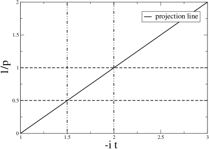
Figure 1: Intersection of the IBS (dash-dotted lines) and BBS thresholds (dashed lines) with the ‘projection line’ (solid line) (18) for $s=3/2$ as an example.

We begin by enforcing the projection condition (18) in the Sutherland equations (11) for the small $p$ regime (12) with (15). This results in:

$$[e_{1}(\lambda_{k})]^{2L}e_{1-2/p}(\lambda_{k})e_{4s+2/p-1}(\lambda_{k})=\prod_{j\neq k}^{N_{h}+N_{\downarrow}}e_{2}(\lambda_{k}-\lambda_{j})e_{2}(\lambda_{k}+\lambda_{j})\times$$

$$\qquad\qquad\times\prod_{\ell=1}^{N_{h}}e_{-1}(\lambda_{k}-\vartheta_{\ell})e_{-1}(\lambda_{k}+\vartheta_{\ell})\,,$$ (20)

$$1=-e_{2/p-2}(\vartheta_{\ell})\prod_{j=1}^{N_{h}+N_{\downarrow}}e_{1}(\vartheta_{\ell}-\lambda_{j})e_{1}(\vartheta_{\ell}+\lambda_{j})\,.$$

Since the Sutherland BA starts from the fully polarized state, in particular the state $|s\rangle_{\mathrm{imp}}$ for the impurity site, the solution to these equations will describe the spectrum of (7), (10) restricted to the spin-$s$ subspace ${\cal H}_{1}$, i.e. that of a Kondo spin $s$ impurity in a correlated $t$–$J$ chain.

Alternatively, we can study the other sector of the impurity Hilbert space selected by the projection scheme, namely ${\cal H}_{2}$ which is the impurity spin $s-1/2$ subspace. In this case, however, the BAE have to be derived from a different pseudo vacuum since the initial state $|s\rangle$ of the impurity used in the Sutherland approach will be discarded by the projection prescription. A possibility to circumvent this problem is to implement the projection condition (18) to the Lai BAE (13) with (14), (16) directly. Here the pseudo vacuum used in the algebraic Bethe ansatz is an element of the projected subspace. Hence, the spectrum of the $\Pi_{2}$ projected impurity is determined by the roots of the Lai-type BAE

$$-[e_{1}(w_{k})]^{2L}e_{4s+2/p-1}(w_{k})=\prod_{\ell=1}^{N_{\downarrow}}e_{1}(w_{k}-x_{\ell})e_{1}(w_{k}+x_{\ell})\,,$$

$$\prod_{j=1}^{N_{e}}e_{1}(x_{\ell}-w_{j})e_{1}(x_{\ell}+w_{j})=e_{2/p}(x_{\ell})e_{2-4s-2/p}(x_{\ell})\times$$ (21)

$$\qquad\qquad\times\prod_{m\neq\ell}^{N_{\downarrow}}e_{2}(x_{\ell}-x_{m})e_{2}(x_{\ell}+x_{m})\,.$$

Up to this point we have made repeated use of the fact that the BAE for the unprojected Hamiltonian in the Sutherland and Lai formulation are related by the $p$–$h$ transformation described in B. Now let us apply the $p$–$h$ transformation to the projected equations to see whether and how this relation manifests itself in the latter. Using Eqs. (33) on the projected Sutherland BAE (20) we obtain the following system of equations in the Lai sector:

$$-[e_{1}(w_{k})]^{2L}e_{4s+2/p-1}(w_{k})=\prod_{\ell=1}^{N_{\downarrow}}e_{1}(w_{k}-x_{\ell})e_{1}(w_{k}+x_{\ell})\,,$$

$$e_{2-2/p}(x_{\ell})\prod_{j=1}^{N_{e}-1}e_{1}(x_{\ell}-w_{j})e_{1}(x_{\ell}+w_{j})=$$ (22)

$$\qquad\qquad=e_{2-4s-2/p}(x_{\ell})\,\prod_{m\neq\ell}^{N_{\downarrow}}e_{2}(x_{\ell}-x_{m})e_{2}(x_{\ell}+x_{m})\,.$$

As expected from our discussion above, these differ from the Lai projected BAE (21). Instead Eqs. (22) are the BAE that one would obtain after populating the charge bound state $w_{0}$ explicitly. Both sets of BAE (20) and (22) can be used for studying the spin-$s$ subspace ${\cal H}_{1}$ of the impurity. The problem of working with a proper pseudo-vacuum in the Lai sector is overcome by enforcing the occupation of the bound state. In fact, Eqs. (22) coincide with the rational limit of the Bethe equations for the $q$-deformed supersymmetric $t$–$J$ model with spin impurities described in terms of singular boundary matrices, i.e. working directly in the projected impurity Hilbert space [42, 43, 44].

Similarly, using Eqs. (33), to map the projected Lai BAE (21) giving the spectrum in the ${\cal H}_{2}$ sector one obtains $p$–$h$ transformed equations for this sector in the Sutherland formulation:

$$[e_{1}(\lambda_{k})]^{2L}e_{-1-2/p}(\lambda_{k})e_{4s+2/p-1}(\lambda_{k})=\prod_{j\neq k}^{N_{h}+N_{\downarrow}}e_{2}(\lambda_{k}-\lambda_{j})e_{2}(\lambda_{k}+\lambda_{j})\times$$

$$\qquad\qquad\times\prod_{\ell=1}^{N_{h}}e_{-1}(\lambda_{k}-\vartheta_{\ell})e_{-1}(\lambda_{k}+\vartheta_{\ell})\,,$$ (23)

$$1=-e_{2/p}(\vartheta_{\ell})\prod_{j=1}^{N_{h}+N_{\downarrow}}e_{1}(\vartheta_{\ell}-\lambda_{j})e_{1}(\vartheta_{\ell}+\lambda_{j})\,.$$

Comparing the boundary phase shifts in these equations we identify those BAE with the ones obtained by occupying the $\lambda_{0}$- and $\vartheta_{0}$-BBS discussed in Section 3.

5 Summary

We have analyzed the role of the bound states appearing in the Bethe ansatz solution for a lattice system with open boundaries. These particular solutions indeed correspond to localized objects at the site of the impurity. As the boundary chemical potential $p$ and the spectral shift $t$ are synchronized according to (18) charge fluctuations are suppressed completely which allows for the projection onto the Hilbert space of a purely magnetic impurity. The equivalence of the Bethe ansätze obtained from different reference states relies on the proper choice of the bound state configurations to select the relevant sector of states as has already been conjectured in [14].

Finally, let us note that the Sutherland equations (20), (23) and similarly the Lai equations (21), (22) for the different impurity sectors of the model are mapped into each other by means of the replacement $1/p\to 1/p+1$ and $s\to s-\frac{1}{2}$. This follows from the fact that the same impurity model can be obtained by projection onto the spin $s-\frac{1}{2}$ sector of either an $[s]_{+}$- or an $[s-\frac{1}{2}]_{+}$-inhomogeneity. Note that the synchronization condition (18) has to be adapted accordingly. To gain additional insight into the underlying algebraic structure of the projection mechanism and the relation between the resulting spin $s$- and $s-\frac{1}{2}$-sectors as well as into the thermodynamical properties of a Kondo-spin coupled to a correlated host the Bethe equations in Section 4 have to be analyzed in more detail. This will be the subject of a forthcoming study.

Appendix A The (super)algebra $gl(2|1)$

Apart from the generators $1$, $S^{z}$, $S^{\pm}$ forming an (ungraded) $gl(2)$ subalgebra, $gl(2|1)$ has an additional generator $B$ of even parity (charge), commuting with the spin operators, and four odd parity generators $V^{\pm}$ and $W^{\pm}$. The commutation relations between even and odd generators are listed below:

$$\begin{array}[]{c}[S^{z},V^{\pm}]=\pm\frac{1}{2}V^{\pm},\qquad[S^{\pm},V^{\pm}]=0,\qquad[S^{\mp},V^{\pm}]=V^{\mp},\\ {[S^{z},W^{\pm}]}=\pm\frac{1}{2}W^{\pm},\qquad[S^{\pm},W^{\pm}]=0,\qquad[S^{\mp},W^{\pm}]=W^{\mp},\\ {[B,V_{\pm}]}=\frac{1}{2}V_{\pm},\qquad[B,W_{\pm}]=-\frac{1}{2}W_{\pm}.\end{array}$$

The odd generators satisfy anticommutation relations

$$\begin{array}[]{c}\{V^{\pm},V^{\pm}\}=\{V^{\pm},V^{\mp}\}=\{W^{\pm},W^{\pm}\}=\{V^{\pm},W^{\mp}\}=0,\\ \{V^{\pm},W^{\pm}\}=\pm\frac{1}{2}S^{\pm},\qquad\{V^{\pm},W^{\mp}\}=\frac{1}{2}(S^{z}\pm B).\end{array}$$

The irreducible representations of $gl(2|1)$ can be classified into typical and atypical ones [23, 24]. With respect to to the even parity $U(1)$ and $SU(2)$ subalgebras they can be decomposed into spin multiplets and are conveniently labelled by the eigenvalues of the even parity operators $B$, $\mathbf{S}^{2}$ and $S^{z}$. The typical $8s$-dimensional representation $[b,s]$ contains four spin-multiplets

$$\begin{array}[]{l}\{|b,s,m\rangle,\,m=-s,\ldots,s\}\,,\\ \{|b,s-1,m\rangle,\,m=-s+1,\ldots,s-1\}\,,\\ \{|b\pm\frac{1}{2},s-\frac{1}{2},m\rangle,\,m=-s+\frac{1}{2},\ldots,s-\frac{1}{2}\}\,.\end{array}$$

As $b\to\pm s$ these representations degenerate into two atypical ones. Atypical representations are denoted by $[s]_{\pm}$ and contain $4s+1$ states in two spin multiplets

$$\begin{array}[]{l}\{|\pm s,s,m\rangle,\,m=-s,\ldots,s\}\,,\\ \{|\pm(s+\frac{1}{2}),s-\frac{1}{2},m\rangle,\,m=-s+\frac{1}{2}),\ldots,s-\frac{1}{2}\}\end{array}$$

respectively. When no confusion is possible we denote the $SU(2)$ highest weight states in the atypical representation $[s]_{+}$ by $|s,s,s\rangle\equiv|s\rangle$ and $|s+\frac{1}{2},s-\frac{1}{2},s-\frac{1}{2}\rangle\equiv|s-\frac{1}{2}\rangle$.

The superalgebra $gl(2|1)$ has two Casimir operators, we have used the quadratic one

$$C_{2}=B^{2}-\mathbf{S}^{2}+W_{-}V_{+}-W_{+}V_{-}+V_{-}W_{+}-V_{+}W_{-}$$ (24)

to express the ${\cal L}$-operator and the Hamiltonian in the main text. On a typical representation $[b,s]$, $C_{2}$ takes the value $b^{2}-s^{2}$ while it vanishes on the atypical ones for any $s$.

Appendix B $p$ – $h$ transformation of the BAE: Lai and Sutherland pseudo vacuua

There are three different BAE for the $gl(2|1)$ supersymmetric $t$–$J$ model depending on the choice of grading in the algebra that contains two fermions and one boson [39]. Here we will focus on two equivalent constructions of the spectrum of the $t$–$J$ model with an $[s]_{+}$-impurity which differ in the choice of the highest-weight state used for the pseudo vacuum in the algebraic Bethe ansatz. Either one can construct the Bethe states starting from the so-called Lai vacuum $|\Omega_{L}\rangle=|0\rangle^{\otimes L}\otimes|s+\frac{1}{2},s-\frac{1}{2},s-\frac{1}{2}\rangle_{imp}$ or from the so-called Sutherland vacuum $|\Omega_{S}\rangle=|\uparrow\rangle^{\otimes L}\otimes|s,s,s\rangle_{imp}$. The two approaches are perfectly equivalent for the description of the system’s spectrum. In the case of the homogeneous chain with periodic boundary conditions, the equivalence of the Lai and Sutherland BAE has been proven in Ref. [38] using a $p$–$h$ transformation introduced by Woynarovich [37]. The aim of this Appendix is to generalize this technique to open boundary conditions including the possibility of having boundary fields and impurity phase shifts. Nevertheless the spirit of the proof is very similar to the one derived in the periodic case.

If one starts from the Sutherland vacuum, the resulting BAE for a $t$–$J$ model with boundaries are given by:

$$[e_{1}(\lambda_{k})]^{2L}\eta(\lambda_{k}) =\prod_{j\neq k}^{N_{h}+N_{\downarrow}}e_{2}(\lambda_{k}-\lambda_{j})e_{2}(\lambda_{k}+\lambda_{j})\prod_{\ell=1}^{N_{h}}e_{-1}(\lambda_{k}-\vartheta_{\ell})e_{-1}(\lambda_{k}+\vartheta_{\ell})\,,$$

$$1 =\xi(\vartheta_{\ell})\prod_{j=1}^{N_{h}+N_{\downarrow}}e_{1}(\vartheta_{\ell}-\lambda_{j})e_{1}(\vartheta_{\ell}+\lambda_{j})\,.$$

where $\eta$ and $\xi$ are phase factors (rational functions in their arguments) describing the boundary and inhomogeneity scattering (see Eqs. (11)). ¿From the second set of these equations we find that $\vartheta_{\ell}$ are zeroes of the polynomial

$$P(w) = \xi_{+}(w)\prod_{j=1}^{N_{h}+N_{\downarrow}}(w-\lambda_{j}+{i\over 2})(w+\lambda_{j}+{i\over 2})$$ (26)

$$-\xi_{-}(w)\prod_{j=1}^{N_{h}+N_{\downarrow}}(w-\lambda_{j}-{i\over 2})(w+\lambda_{j}-{i\over 2})\equiv 0.$$

Here $\xi_{+}$ (resp. $\xi_{-}$) stands for the numerator (resp. denominator) of the function $\xi$. $P(w)$ is of degree $2(N_{h}+N_{\downarrow})+\delta$ where $\delta$ is determined by the degree and the parity of $\xi_{\pm}(w)$. Hence, in addition to the first $2N_{h}$ roots of $P(w)$ which we identify with the roots $\{\vartheta_{\ell}\}$ of the BAE (LABEL:Sub) there are $2N_{\downarrow}+\delta$ additional zeroes $\{x_{\ell}\}$. Notice that $P(w)$ is an odd polynomial in all cases considered in this paper. Consequently, the zeroes of $P$ come in pairs $\vartheta_{\ell}=-\vartheta_{-\ell}$ and $x_{\ell}=-x_{-\ell}$ except from a single root at $x_{0}=0$. Using the residue theorem we obtain:

$$\sum_{\ell=1}^{N_{h}}{1\over i}\ln\left(\frac{\lambda_{k}-\vartheta_{\ell}-{i\over 2}}{\lambda_{k}-\vartheta_{\ell}+{i\over 2}}\frac{\lambda_{k}+\vartheta_{\ell}-{i\over 2}}{\lambda_{k}+\vartheta_{\ell}+{i\over 2}}\right)=\sum_{\ell=1}^{N_{h}}\frac{1}{2\pi i}\oint_{{\cal C}_{\ell}}\mathrm{d}z{1\over i}\ln\left(\frac{\lambda_{k}-z-{i\over 2}}{\lambda_{k}-z+{i\over 2}}\right)\frac{\mathrm{d}}{\mathrm{d}z}\ln P(z)=$$

(27)

$$=-\sum_{\ell=1}^{N_{\downarrow}}{1\over i}\ln\left(\frac{\lambda_{k}-x_{\ell}-{i\over 2}}{\lambda_{k}-x_{\ell}+{i\over 2}}\,\frac{\lambda_{k}+x_{\ell}-{i\over 2}}{\lambda_{k}+x_{\ell}+{i\over 2}}\right)-{1\over i}\ln\left(\frac{\lambda_{k}-{i\over 2}}{\lambda_{k}+{i\over 2}}\right)+{1\over i}\ln\left(\frac{P(\lambda_{k}-{i\over 2})}{P(\lambda_{k}+{i\over 2})}\right)$$

(the last sum runs over the nonzero $x_{\ell}$). The contour ${\cal C}_{\ell}$ is chosen such that it encloses both zeroes $\vartheta_{\ell}$ and $-\vartheta_{\ell}$ carefully avoiding the logarithm’s branch cut between $\lambda_{k}-i/2$ and $\lambda_{k}+i/2$ (see Fig. 2).

Figure 2: The Contour ${\cal C}_{\ell}$ used in Eq. (27) encloses the points $\vartheta_{\ell}$ and $-\vartheta_{\ell}$. The branch cut of the logarithm in the integrand is depicted as the dashed line connecting from $\lambda_{k}-i/2$ to $\lambda_{k}+i/2$.

By definition of $P$ (26) we evaluate its value at both ends of the branch cuts,

$$P(\lambda_{k}-{i\over 2}) = -\xi_{-}(\lambda_{k}-{i\over 2})\prod_{j=1}^{N_{h}+N_{\downarrow}}(\lambda_{k}-\lambda_{j}-i)(\lambda_{k}+\lambda_{j}-i)\,,$$

$$P(\lambda_{k}+{i\over 2}) = \xi_{+}(\lambda_{k}+{i\over 2})\prod_{j=1}^{N_{h}+N_{\downarrow}}(\lambda_{k}-\lambda_{j}+i)(\lambda_{k}+\lambda_{j}+i)\,.$$

Exponentiating Eq. (27) we obtain

$$\prod_{\ell=1}^{N_{h}}e_{-1}(\lambda_{k}-\vartheta_{\ell})e_{-1}(\lambda_{k}+\vartheta_{\ell})=-e_{1}(\lambda_{k})\,\frac{\xi_{-}(\lambda_{k}-{i\over 2})}{\xi_{+}(\lambda_{k}+{i\over 2})}\times$$

$$\quad\times\prod_{\ell=1}^{N_{\downarrow}}e_{1}(\lambda_{k}-x_{\ell})e_{1}(\lambda_{k}+x_{\ell})\,\prod_{j=1}^{N_{h}+N_{\downarrow}}e_{-2}(\lambda_{k}-\lambda_{j})e_{-2}(\lambda_{k}+\lambda_{j})\,.$$ (29)

The last product appearing on the r.h.s. can be reexpressed as

$$\prod_{j=1}^{N_{h}+N_{\downarrow}}e_{-2}(\lambda_{k}-\lambda_{j})e_{-2}(\lambda_{k}+\lambda_{j})=-e_{-1}(\lambda_{k})\prod_{j\neq k}^{N_{h}+N_{\downarrow}}e_{-2}(\lambda_{k}-\lambda_{j})e_{-2}(\lambda_{k}+\lambda_{j})$$ (30)

since $e_{-2}(2\lambda_{k})=e_{-1}(\lambda_{k})$. Then, using Eq. (29) in the first of Eqs. (LABEL:Sub) we obtain:

$$\eta(\lambda_{k})[e_{1}(\lambda_{k})]^{2L}=\frac{\xi_{-}(\lambda_{k}-{i\over 2})}{\xi_{+}(\lambda_{k}+{i\over 2})}\,\prod_{\ell=1}^{N_{\downarrow}}e_{1}(\lambda_{k}-x_{\ell})e_{1}(\lambda_{k}+x_{\ell})\,$$ (31)

(cf. the first of the Lai equations (13)). Starting from Eq. (31), it is straightforward to apply the same procedure as before to derive the second Lai type equation.

To summarize the main result of this Appendix let us write the relation connecting the boundary phase factors within BAE in the Sutherland representation (LABEL:Sub) and those in the Lai representation:

$$\Phi(w_{k})[e_{1}(w_{k})]^{2L}=\prod_{\ell=1}^{N_{\downarrow}}e_{1}(w_{k}-x_{\ell})e_{1}(w_{k}+x_{\ell}),$$

(32)

$$\Xi(x_{\ell})\prod_{j=1}^{N_{e}}e_{1}(x_{\ell}-w_{j})e_{1}(x_{\ell}+w_{j})=\prod_{m\neq\ell}^{N_{\downarrow}}e_{2}(x_{\ell}-x_{m})e_{2}(x_{\ell}+x_{m}).$$

Comparing the result of the particle-hole transformation applied to (LABEL:Sub) with (32) we find

$$\eta(\lambda)\frac{\xi_{+}(\lambda+{i\over 2})}{\xi_{-}(\lambda-{i\over 2})}=\Phi(\lambda)\,,\qquad\xi^{-1}(x)=\Xi(x)\frac{\Phi_{-}(x+{i\over 2})}{\Phi_{+}(x-{i\over 2})}\,.$$ (33)

References

References

- [1] A. C. Hewson, The Kondo Problem to Heavy Fermions (Cambridge University Press, Cambridge, 1993).
- [2] D.-H. Lee and J. Toner, Phys. Rev. Lett. 69, 3378 (1992).
- [3] A. Furusaki and N. Nagaosa, Phys. Rev. Lett. 72, 892 (1994).
- [4] P. Fröjdh and H. Johannesson, Phys. Rev. Lett. 75, 300 (1995).
- [5] R. Egger and A. Komnik, Phys. Rev. B 57, 10620 (1998).
- [6] A. M. Tsvelick and P. W. Wiegmann, Adv. Phys. 32, 453 (1983).
- [7] N. Andrei, K. Furuya, and J. H. Lowenstein, Rev. Mod. Phys. 55, 331 (1983).
- [8] N. Andrei and H. Johannesson, Phys. Lett. A 100, 108 (1984).
- [9] G. Bedürftig, F. H. L. Eßler, and H. Frahm, Phys. Rev. Lett. 77, 5098 (1996).
- [10] G. Bedürftig, F. H. L. Eßler, and H. Frahm, Nucl. Phys. B 489, 697 (1997).
- [11] P. Schlottmann and A. A. Zvyagin, Phys. Rev. B 55, 5027 (1997).
- [12] M. Bortz, A. Klümper, and C. Scheeren, Phys. Rev. B 71, 144421 (2005).
- [13] H. Frahm and A. A. Zvyagin, J. Phys. Condens. Matter 9, 9939 (1997).
- [14] G. Bedürftig and H. Frahm, J. Phys. A 32, 4585 (1999).
- [15] Y. Wang, J.-H. Dai, Z.-N. Hu, and F.-C. Pu, Phys. Rev. Lett. 79, 1901 (1997).
- [16] J.-H. Dai and Y. Wang, cond-mat/9809008.
- [17] H.-Q. Zhou and M. D. Gould, Phys. Lett. A 251, 279 (1999).
- [18] H.-Q. Zhou, X.-Y. Ge, J. Links, and M. D. Gould, Nucl. Phys. B 546, 779 (1999).
- [19] I. V. Cherednik, Theor. Math. Phys. 61, 977 (1984).
- [20] E. K. Sklyanin, J. Phys. A 21, 2375 (1988).
- [21] H. Frahm and N. A. Slavnov, J. Phys. A 32, 1547 (1999).
- [22] V. E. Korepin, N. M. Bogoliubov, and A. G. Izergin, Quantum Inverse Scattering Method and Correlation Functions (Cambridge University Press, Cambridge, 1993).
- [23] M. Scheunert, W. Nahm, and V. Rittenberg, J. Math. Phys. 18, 155 (1977).
- [24] M. Marcu, J. Math. Phys. 21, 1277 (1980).
- [25] H. Frahm, M. P. Pfannmüller, and A. M. Tsvelik, Phys. Rev. Lett. 81, 2116 (1998).
- [26] H. Frahm, Nucl. Phys. B 559, 613 (1999).
- [27] H. Frahm and N. A. Slavnov, Nucl. Phys. B 575 [FS], 485 (2000).
- [28] P. P. Kulish, J. Sov. Math. 35, 2648 (1986), [Zap. Nauch. Semin. LOMI 145, 140 (1985)].
- [29] F. H. L. Eßler, J. Phys. A 29, 6183 (1996).
- [30] A. González-Ruiz, Nucl. Phys. B 424, 468 (1994).
- [31] F. H. L. Eßler and H. Frahm, Phys. Rev. B 56, 6631 (1997).
- [32] H. Frahm and G. Palacios, Phys. Rev. B 73, 214419 (2006).
- [33] B. Sutherland, Phys. Rev. B 12, 3795 (1975).
- [34] S. Skorik and H. Saleur, J. Phys. A 28, 6605 (1995).
- [35] A. Kapustin and S. Skorik, J. Phys. A 29, 1629 (1996).
- [36] C. K. Lai, J. Math. Phys. 15, 1675 (1974).
- [37] F. Woynarovich, J. Phys. C 16, 6593 (1983).
- [38] P.-A. Bares, J. M. P. Carmelo, J. Ferrer, and P. Horsch, Phys. Rev. B 46, 14624 (1992).
- [39] F. H. L. Eßler and V. E. Korepin, Phys. Rev. B 46, 9147 (1992).
- [40] F. Göhmann and H. Schulz, J. Phys. Condens. Matter 2, 3841 (1990).
- [41] Y. Wang and J. Voit, Phys. Rev. Lett. 77, 4934 (1996).
- [42] H. Fan, M. Wadati, and R. Yue, J. Phys. A 33, 6187 (2000).
- [43] H. Fan and M. Wadati, Nucl. Phys. B 599, 561 (2001).
- [44] X.-Y. Ge, M. D. Gould, and H.-Q. Zhou, J. Phys. A 34, 8543 (2001).