Effect of symmetry on the electronic structure of spheroidal fullerenes in a weak uniform magnetic field

Abstract

The effect of a weak uniform magnetic field on the electronic structure of slightly deformed fullerene molecules is studied within the continuum field-theory model. It is shown that fine structure of the electronic energy spectrum is very sensitive to the orientation of the magnetic field. In particular, we found that the magnetic field pointed in the x direction does not influence the first electronic level whereas it causes a splitting of the second energy level. This behavior differs markedly from the case of the magnetic field pointed in the z direction.

I Introduction

Recently, we have considered the problem of the low energy electronic states in spheroidal fullerenes Pudlak1 as well as the influence of a weak uniform external magnetic field pointed in the z direction Pudlak2 . The main findings were a discovery of fine structure with a specific shift of the electronic levels upwards due to spheroidal deformation and the Zeeman splitting of electronic levels due to a weak uniform magnetic field. In addition, it was shown that the external magnetic field modifies the density of electronic states and does not change the number of zero modes. In this paper, we examine the case of the magnetic field pointed in the x direction. It is interesting to note that the obtained modification of the electronic spectrum of the spheroidal fullerenes differs markedly from the case of the z-directed magnetic field. The reason is the proper symmetry of the spheroid, which changes the role of the external magnetic field in comparison with the spherical case. This gives an additional possibility for experimental study of the electronic structure of deformed fullerene molecules.

Notice that the Schrödinger equation for a free electron on the surface of a sphere in a uniform magnetic field was formulated and solved to describe Zeeman splitting and Landau quantization of electrons on a sphere in Ref. Aoki . We have explored in the Ref. Pudlak2 the field-theory model where the specific structure of carbon lattice, geometry, and the topological defects (pentagons) were taken into account. Following the Euler’s theorem one has to insert twelve pentagons into hexagonal network in order to form the closed molecules. In the framework of continuum description we extend the Dirac operator by introducing the Dirac monopole field inside the spheroid to simulate the elastic vortices due to twelve pentagonal defects. The exchange of two different Dirac spinors which describes the K spin flux in the presence of a conical singularity is included in a form of t’Hooft-Polyakov monopole. Our studies cover slightly elliptically deformed molecules in a weak uniform external magnetic field pointed in the x directions.

II The model and the results

Spheroidal fullerenes can be considered as an initially flat hexagonal network which has been wrapped into closed monosurface by using of twelve disclinations Kroto . We start from the tight-binding model of graphite layer with the trial wave function taken in the form

$$\chi(\vec{r})=\psi_{A}(\vec{r})\chi_{A}(\vec{K},\vec{r})+\psi_{B}(\vec{r})\chi_{B}(\vec{K},\vec{r}).$$ (1)

As is seen, the trial function is described by smoothly varying envelope functions $\psi_{A,B}(\vec{r})$ multiplying by the Bloch functions $\chi_{A,B}(\vec{K},\vec{r})$. Within the $\vec{k}\vec{p}$ approximation one obtains the equations algebraically identical to a two-dimensional Dirac equations, where two component wave function $\psi$ represents graphite sublattices $A$ and $B$. Following the approach developed in Gonzales ; Osipov let us write down the Dirac operator for free massless fermions on the Riemannian spheroid $S^{2}$. The Dirac equation on a surface $\Sigma$ in the presence of the abelian magnetic monopole field $W_{\mu}$ and the external magnetic field $A_{\mu}$ is written as Davies

$$i\gamma^{\alpha}e_{\alpha}^{\ \mu}[\nabla_{\mu}-iW_{\mu}-iA_{\mu}]\psi=E\psi,$$ (2)

where $e_{\alpha}^{\mu}$ is the zweibein, $g_{\mu\nu}=e^{\alpha}_{\mu}e^{\beta}_{\nu}\delta_{\alpha\beta}$ is the metric, the orthonormal frame indices $\alpha,\beta=\{1,2\}$, the coordinate indices $\mu,\nu=\{1,2\}$, and $\nabla_{\mu}=\partial_{\mu}+\Omega_{\mu}$ with

$$\Omega_{\mu}=\frac{1}{8}\omega^{\alpha\ \beta}_{\ \mu}[\gamma_{\alpha},\gamma_{\beta}],$$ (3)

being the spin connection term in the spinor representation (see Nakahara ; Gockeler for details). The energy in (2) is measured from the Fermi level.

The model (3) allows us to study the structure of electron levels near the Fermi energy. It is convenient to consider this problem by using of the Cartesian coordinates $x$, $y$, $z$ in the form

$$x=a~{}\sin\theta\cos\phi;\quad y=a~{}\sin\theta\sin\phi;\quad z=c~{}\cos\theta.$$ (4)

The Riemannian connection reads (cf. (4))

$$\omega{{}_{\phi 2}^{1}}=-\omega{{}_{\phi 1}^{2}}=\frac{a\cos\theta}{\sqrt{a^{2}\cos^{2}\theta+c^{2}\sin^{2}\theta}}\ ;\quad\omega{{}_{\theta 2}^{1}}=\omega{{}_{\theta 1}^{2}}=0.$$ (5)

Within the framework of the perturbation scheme the spin connection coefficients are written as

$$\omega{{}_{\phi 2}^{1}}=-\omega{{}_{\phi 1}^{2}}\approx\cos\theta(1-\delta\sin^{2}\theta),$$ (6)

where $c=a+\delta a$ and the terms to first order in $\delta$ are taken into account. In spheroidal coordinates, the only nonzero component of $W_{\mu}$ in region $R_{N}$ is found to be (see Ref. Pudlak1 )

$$W_{\phi}\approx g\cos\theta(1+\delta\sin^{2}\theta)+G(1-\cos\theta)-\delta G\sin^{2}\theta\cos\theta.$$ (7)

The external magnetic field $B$ is chosen to be pointed in the $x$ direction, so that $\vec{A}=B\left(0,-z,y\right)/2$. One obtains

$$A_{\phi}=-\frac{1}{2}Bac\sin\theta\cos\theta\cos\phi,$$ (8)

$$A_{\theta}=-\frac{1}{2}Bac\sin\phi.$$ (9)

The Dirac matrices can be chosen to be the Pauli matrices, $\gamma_{1}=-\sigma_{2},\gamma_{2}=-\sigma_{1}$. By using the substitution

$$\left(\begin{array}[]{c}\psi_{A}\\ \psi_{B}\\ \end{array}\right)=\sum_{j}\frac{e^{i(j+G)\phi}}{\sqrt{2\pi}}\left(\begin{array}[]{c}u_{j}(r)\\ v_{j}(r)\\ \end{array}\right),j=0,\pm 1,\pm 2,\ldots$$ (10)

we obtain the Dirac equation for functions $u_{j}$ and $v_{j}$ in the form

$$\left(-i\sigma_{1}\frac{1}{a}(\partial_{\theta}+\frac{\cot\theta}{2}+i\frac{1}{2}Ba^{2}\sin\phi)+\frac{\sigma_{2}}{a\sin\theta}\left(j-m\cos\theta+\frac{1}{2}Ba^{2}\sin\theta\cos\theta\cos\phi\right)+\delta\hat{\cal{D}}_{1}\right)\times$$

$$\times\left(\begin{array}[]{c}u_{j}(\theta)\\ v_{j}(\theta)\\ \end{array}\right)=E\left(\begin{array}[]{c}u_{j}(\theta)\\ v_{j}(\theta)\\ \end{array}\right),$$ (11)

where

$$\hat{\cal{D}}_{1}=-\frac{\gamma_{1}}{a}\sin\theta\left(j-2m\cos\theta\right)-\gamma_{1}\frac{Ba}{2}\sin^{2}\theta\cos\theta\cos\phi.$$ (12)

The square of nonperturbative part of Dirac operator takes the form

$$\hat{\cal{D}}_{0}^{2} = -\frac{1}{a^{2}}\left(\partial^{2}_{\theta}+\frac{\cos\theta}{\sin\theta}\partial_{\theta}-\frac{1}{4}-\frac{1}{4\sin^{2}\theta}\right)+\frac{\left(j-m\cos\theta\right)^{2}}{a^{2}\sin^{2}\theta}$$ (13)

$$+\sigma_{3}\frac{m-j\cos\theta}{a^{2}\sin^{2}\theta}+BV(\theta,\phi).$$

Notice that in (11)-(13) the terms with $B^{2}$ and $\delta B$ were neglected and

$$V(\theta,\phi) = -i(\cos\phi\partial_{\phi}-\frac{\sin\phi}{2})\cot\theta-\sigma_{3}\frac{\cos\phi(1+\sin^{2}\theta)}{2\sin\theta}-i(\partial_{\theta}+\frac{1}{2}\cot\theta)\sin\phi$$ (14)

$$-\frac{m\cos^{2}\theta\cos\phi}{\sin\theta}.$$

Let us define $V_{j,j^{\prime}}^{m}=\langle\psi_{jn}^{m}|V(\theta,\phi)|\psi_{j^{\prime}n}^{m}\rangle$, where $\psi_{jn}^{m}$ are the eigenfunctions of $\hat{\cal{D}}_{0}$. In the case of the first energy mode the terms $V_{-1,-1}^{1/2}$, $V_{1,1}^{1/2}$, $V_{1,-1}^{1/2}$, $V_{-1,1}^{1/2}$ are found to be zero and, therefore, the weak magnetic field pointed in the x direction does not influence the first energy level. For the second energy mode, only non-diagonal terms $V_{-1,-2}^{1/2}$, $V_{1,2}^{1/2}$ differ from zero with $V_{-1,-2}^{1/2}=-2.1$ and $V_{1,2}^{1/2}=2.1$. Notice that the following wave functions were used for calculations of non-diagonal terms:

$$\psi_{0,2}^{1/2}(z,\phi)=\frac{e^{i2\phi}}{\sqrt{2\pi}}\sqrt{\frac{32}{15}}\left(\begin{array}[]{c}-i\sqrt{\frac{2}{3}}\sqrt{1-z^{2}}(1+z)\\ 1-z^{2}\\ \end{array}\right),$$ (17)

$$\psi_{0,-2}^{1/2}(z,\phi)=\frac{e^{-i2\phi}}{\sqrt{2\pi}}\sqrt{\frac{32}{15}}\left(\begin{array}[]{c}i\sqrt{\frac{2}{3}}\sqrt{1-z^{2}}(1-z)\\ 1-z^{2}\\ \end{array}\right),$$ (20)

$$\psi_{1,1}^{1/2}(z,\phi)=\frac{e^{i\phi}}{\sqrt{2\pi}}\sqrt{\frac{3}{5}}\left(\begin{array}[]{c}-i\sqrt{\frac{2}{3}}(2z^{2}+z-1)\\ \frac{3}{2}z\sqrt{1-z^{2}}\\ \end{array}\right),$$ (23)

$$\psi_{1,-1}^{1/2}(z,\phi)=\frac{e^{-i\phi}}{\sqrt{2\pi}}\sqrt{\frac{3}{5}}\left(\begin{array}[]{c}i\sqrt{\frac{2}{3}}(-2z^{2}+z+1)\\ \frac{3}{2}z\sqrt{1-z^{2}}\\ \end{array}\right).$$ (26)

The low energy electronic spectrum of spheroidal fullerenes in this case takes the form

$$E_{jn}=E^{0}_{jn}+E^{\delta B_{x}},$$ (27)

where

$$E^{\delta B_{x}}=\frac{\delta\left(\hat{\Gamma}_{22}+\hat{\Gamma}_{11}\right)\pm\sqrt{\delta^{2}\left(\hat{\Gamma}_{22}-\hat{\Gamma}_{11}\right)^{2}+4|Ba^{2}V_{1,2}|^{2}}}{4E^{0}_{jn}}.$$ (28)

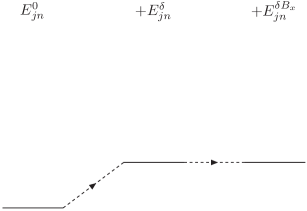
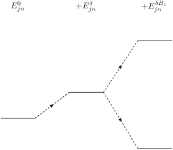
Figure 1: The schematic picture of the first electronic level $E_{jn}$ of spheroidal fullerenes in a weak uniform magnetic field pointed in the x (left) and z (right) directions.

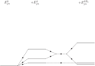
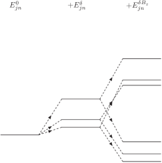
Figure 2: The schematic picture of the second electronic level $E_{jn}$ of spheroidal fullerenes in a weak uniform magnetic field pointed in the x (left) and z (right) directions.

Here $\hat{\Gamma}_{ii}$ are the diagonal matrix elements (see Ref. Pudlak2 ). Table 1 shows contributions to the first and second energy levels for YO-C₂₄₀ (YO means a structure given in yoshida ; Lu ). As is seen, there is a marked difference between the behavior of the first and second energy levels in magnetic field. Indeed, in both cases the energy levels become shifted due to spheroidal deformation. However, the uniform magnetic field does not influence the first energy level. The splitting takes place only for the second level. This is clearly illustrated in Fig. 1 and Fig.2, which schematically show the structure of the first and second levels in the uniform magnetic field pointed in x direction. The case of the z-directed magnetic field is also shown for comparison. We can conclude that there is a possibility to change the structure of the electronic levels in spheroidal fullerenes by altering the direction of magnetic field. It would be interesting to test this prediction in experiment.

III The $SU(2)$ algebra

To gain a better understanding of the difference between the spheroidal and spherical cases, let us consider the angular-momentum operators for Dirac operator on the sphere $S^{2}$ with charge $G$ and a total magnetic monopole $m$

$$\hat{L}_{z}=-i(\partial_{\phi}\mp iG),$$ (29)

$$\hat{L}_{x}=i\sin\phi\partial_{\theta}+i\cos\phi\frac{\cos\theta}{\sin\theta}\left(\partial_{\phi}\mp iG-i\frac{m}{\cos\theta}\right)+\sigma_{z}\frac{\cos\phi}{2\sin\theta},$$ (30)

$$\hat{L}_{y}=-i\cos\phi\partial_{\theta}+i\sin\phi\frac{\cos\theta}{\sin\theta}\left(\partial_{\phi}\mp iG-i\frac{m}{\cos\theta}\right)+\sigma_{z}\frac{\sin\phi}{2\sin\theta}.$$ (31)

Here $-(+)$ signs correspond to the case of north (south) hemisphere, respectively. These operators satisfy the standard commutations relations of the $SU(2)$ algebra

$$\varepsilon_{ijk}\hat{L}_{j}\hat{L}_{k}=i\hat{L}_{i}.$$ (32)

For zero magnetic field, the square of the Dirac operator and $\hat{L}^{2}$ may be diagonalized simultaneously

$$\hat{\cal{D}}_{0}^{2}(B=0)=\hat{L}^{2}+\frac{1}{4}-m^{2}.$$ (33)

For the magnetic field pointed in the z direction, the operator $V(\theta,\phi)$ can be expressed in the form

$$V(\theta,\phi)=\hat{L_{z}}+\left(\frac{\sigma_{3}}{2}-m\right)z,$$ (34)

while in the case of the magnetic field pointed in the x direction one obtains

$$V(\theta,\phi)=-\hat{L_{x}}-\left(\frac{\sigma_{3}}{2}-m\right)x.$$ (35)

Here $x$ and $z$ are the Cartesian coordinates: $x=\sin\theta\cos\phi;\quad z=\cos\theta$. In this case, the square of the Dirac operator and operator $\hat{L}^{2}$ may also be diagonalized simultaneously and their eigenvalues are interrelated

$$\langle E,n|\hat{L}^{2}|E,n\rangle=l(l+1)=E^{2}-\frac{1}{4}=(n+|j|)(n+|j|+1),$$ (36)

where $l=n+|j|$. The eigenstates of $\hat{\cal{D}}_{0}(B=0)$ have the form

$$\Psi_{l,j}(x,\phi)=\frac{e^{i(j\pm G)\phi}}{\sqrt{2\pi}\Omega}\sqrt{\frac{(l+j)!}{(l-j)!}}$$

$$\times\left(\begin{array}[]{c}(1-x)^{-\frac{1}{2}(j-m-1/2)}(1+x)^{-\frac{1}{2}(j+m+1/2)}\frac{d^{l-j}}{dx^{l-j}}(1-x)^{(l-m-1/2)}(1+x)^{(l+m+1/2)}\\ isgn(E)(1-x)^{-\frac{1}{2}(j-m+1/2)}(1+x)^{-\frac{1}{2}(j+m-1/2)}\frac{d^{l-j}}{dx^{l-j}}(1-x)^{(l-m+1/2)}(1+x)^{(l+m-1/2)}\end{array}\right)$$ (37)

where $\Omega=2^{l}\sqrt{\Gamma(l-m+1/2)^{2}+\Gamma(l+m+1/2)^{2}}$ where $\Gamma$ are the Gamma functions (see Ref. Abrikosov ). One can introduce the operators $\hat{L}_{-}$ and $\hat{L}_{+}$ so that

$$\hat{L}_{-}\Psi_{l,j}=\sqrt{(l+j)(l-j+1)}\Psi_{l,j-1},$$ (38)

$$\hat{L}_{+}\Psi_{l,j}=\sqrt{(l+j+1)(l-j)}\Psi_{l,j+1},$$ (39)

with

$$\hat{L}_{-}=-e^{-i\phi}\left(\partial_{\theta}-i\frac{\cos\theta}{\sin\theta}\left(\partial_{\phi}\mp iG-i\frac{m}{\cos\theta}\right)-\frac{\sigma_{z}}{2\sin\theta}\right),$$ (40)

$$\hat{L}_{+}=e^{i\phi}\left(\partial_{\theta}+i\frac{\cos\theta}{\sin\theta}\left(\partial_{\phi}\mp iG-i\frac{m}{\cos\theta}\right)+\frac{\sigma_{z}}{2\sin\theta}\right).$$ (41)

Let us transform these expressions to the Cartesian coordinates. The corresponding transformation rules for spinors are Abrikosov

$$(\Psi)_{C}=V^{{\dagger}}\Psi,$$ (42)

and the Cartesian realization of operator $\hat{L}$ is

$$\hat{L}_{C}=V^{{\dagger}}\hat{L}V,$$ (43)

with

$$V=\exp\left(\frac{i\sigma_{y}}{2}\theta\right)\exp\left(\frac{i\sigma_{z}}{2}\phi\right).$$ (44)

For example, the Cartesian realization of $\hat{L}_{x}$ takes the form

$$(\hat{L}_{x})_{C}=i\sin\phi\partial_{\theta}+i\cos\phi\frac{\cos\theta}{\sin\theta}\left(\partial_{\phi}\mp iG-i\frac{m}{\cos\theta}\right)+\frac{\sigma_{x}}{2}.$$ (45)

For $m=G=0$ it may be written in the well-known form

$$(\hat{L}_{x})_{C}=y\hat{p}_{z}-z\hat{p}_{y}+\frac{\sigma_{x}}{2}.$$ (46)

IV Conclusion

We have studied the influence of the uniform magnetic field on the energy levels of spheroidal fullerenes. The case of the x-directed magnetic field was considered and compared with the case of the z-th direction. The z axis is defined as the rotational axis of the spheroid with maximal symmetry. The most important finding is that the splitting of the electronic levels depends on the direction of the magnetic field. Our consideration was based on the using of the eigenfunctions of the Dirac operator on the spheroid, which are also the eigenfunction of $\hat{L}_{z}$. Let us discuss this important point in more detail.

In the case of a sphere there is no preferable direction in the absence of the magnetic field. The magnetic field sets a vector, so that the z-axis can be oriented along the field. In this case, one has to use such eigenfunctions of the Dirac operator which are also the eigenfunctions of $\hat{L}_{z}$. For the x-directed magnetic field, the eigenfunction of both the Dirac operator and $\hat{L}_{x}$ must be used. Evidently, the same results will be obtained in both cases.

The situation differs markedly for a spheroid. The spheroidal symmetry itself assumes the preferential direction which can be chosen as the z-axis. In other words, the external magnetic field does not define the preferable orientation. The symmetry is already broken and, as a result, the case of the magnetic field pointed in the $x$ direction differs from the case of the $z$-directed field. For instance, there are no eigenfunctions which would be simultaneously the eigenfunctions of both the Dirac operator on the spheroid and $\hat{L}_{x}$. For this reason, the structure of the electronic levels is found to crucially depend on the direction of the external magnetic field.

The work was supported in part by VEGA grant 2/7056/27. of the Slovak Academy of Sciences, by the Science and Technology Assistance Agency under contract No. APVT-51-027904 and by the Russian Foundation for Basic Research under Grant No. 05-02-17721.

$YO-C_{240}$	$j$	$E^{0}_{jn}(eV)$	$E_{jn}^{\delta}(meV)(B=0)$	$E_{jn}^{\delta B_{x}}(meV)(Ba^{2}=0.1)$
$n=0$, $m=1/2$	1	1.094	10.5	10.5
	-1	1.094	10.5	10.5
$n=0$, $m=-5/2$	3	1.89	3	3
	-3	1.89	3	3
$n=0$, $m=1/2$	2	1.89	28.4
				53/-16/
$n=1$	1	1.89	8.8
$n=1$, $m=1/2$	-1	1.89	8.8
				53/-16/
$n=0$	-2	1.89	28.4

Table 1: The structure of the first and second energy levels for YO-C₂₄₀ fullerene in uniform magnetic field. The hopping integral and other parameters are taken to be $t=2.5\ eV$ and $V_{F}=3t\overline{b}/2\hbar$, $\overline{b}=1.45{\textmd{\AA}}$, $\overline{R}=7.03{\textmd{\AA}}$, $SD=0.17{\textmd{\AA}}$, $\delta=0.024$. $\overline{b}$ is average bond length, $\overline{R}\ (\overline{R}=a)$ is average radius, $SD$ is standard deviation from a perfect sphere (see Refs. [10,11]), so that $\delta=SD/\overline{R}$.

References

- (1) M. Pudlak, R. Pincak and V.A. Osipov, Phys. Rev. B 74 (2006) 235435.
- (2) M. Pudlak, R. Pincak and V.A. Osipov, Phys. Rev. A 75 (2007) 025201.
- (3) H. Aoki and H. Suezawa, Phys. Rev. A 46 (1992) R1163.
- (4) H. Kroto, Rev.Mod.Phys. 69 (1997) 703.
- (5) J. Gonzales, F. Guinea and F.A.H. Vozmediano, Nucl.Phys.B 406 (1993) 771.
- (6) D.V. Kolesnikov and V.A. Osipov, Eur.Phys.Journ. B 49 (2006) 465.
- (7) N.D. Birrell and P.C.W. Davies, Quantum Fields in Curved Space, (Cambridge 1982).
- (8) M. Nakahara, Geometry, Topology and Physics, (Institute of Physics Publishing Bristol 1998).
- (9) M.Göckeler and T.Schücker, Differential geometry, gauge theories, and gravity (Cambridge University Press 1989).
- (10) M. Yoshida and E. Osawa, Fullerene Sci. Tech. 1 (1993) 55.
- (11) J. P. Lu and W. Yang, Phys. Rev. B 49 (1994) 11421.
- (12) A.A. Abrikosov jr., Int. Journ. of Mod. Phys. A 17 (2002) 885.