Driving particle current through narrow channels using classical pump

Abstract

We study a symmetric exclusion process in which the hopping rates at two chosen adjacent sites vary periodically in time and have a relative phase difference. This mimics a colloidal suspension subjected to external time dependent modulation of the local chemical potential. The two special sites act as a classical pump by generating an oscillatory current with a nonzero ${\cal DC}$ value whose direction depends on the applied phase difference. We analyze various features in this model through simulations and obtain an expression for the $\cal{DC}$ current via a novel perturbative treatment.

A number of studies have used the idea of Thouless adiabatic pumping Thouless (1983) to generate $\cal{DC}$ current responses to $\cal{AC}$ driving fields in quantum systems. This mechanism has been used experimentally to generate charge Switkes et al. (1999) and spin Watson et al. (2003) current in systems such as quantum dots and nanotubes and studied theoretically in various quantum systems without Brouwer:1998 and with Aleiner and Andreev (1998) interactions. One may ask if this principle can be used to drive current in classical systems. It was shown in Moskalets:2001 that inelastic scattering can enhance pumping which suggests that similar effects can be obtained in purely classical systems. Indeed classical pumping of particles and heat has been achieved in mesoscopic systems with large inelastic scattering Moskalets:2001 , stochastic models Astumian:2001 ; Marathe:2007 ; Sinitsyn:2007 and seen in experiments Astumian:2003 . As discussed in astumian02 these pump models are similar to Brownian ratchets Reimann (2002) where non-interacting particles placed in spatially asymmetric potentials that vary periodically in time and acted upon by noise execute directed motion. However for the model described below, particle interactions seem necessary for pumping.

Here we show how the designing principle of quantum pumps may be applied to drive classical particles such as micron-sized charged colloidal particles confined in a closed narrow tube. Systems of colloidal particles with excluded volume interactions diffusing in a narrow channel have been modeled in the recent past Chou (1998); Wei et al. (2000) by one-dimensional symmetric exclusion process (SEP) in which hard-core particles attempt to hop to an empty neighbor with equal rate Liggett (1985). Recently much attention has been given to nonequilibrium steady states of driven SEP Spohn (1983); Santos and Schütz (2001), in which particles can enter or leave the system at the boundaries, to study large deviation functional Derrida et al. (2002) and current fluctuations Derrida et al. (2004) in nonequilibrium systems.

In this Letter, we introduce a SEP in which the hop-out rates at some lattice sites are chosen to be time-dependent with a relative phase difference between different points. At a coarse-grained level, this choice models oscillating voltages applied to the colloidal system. We find that an oscillatory particle current is generated across a bond which interestingly has a nonzero $\mathcal{DC}$ value. Unlike driven SEP, our model conserves the total number of particles and due to the periodically varying hopping rates, the system reaches in the long time limit a periodic time-dependent state.

Here we will mainly focus on the model with a single pump which we define as consisting of two adjacent sites where the hopping rates vary periodically and with a phase difference. The hopping rate at all other sites is constant. Our Monte-Carlo simulations indicate that the magnitude of the $\mathcal{DC}$ current $\bar{J}$ depends sinusoidally on the phase difference between the rates at these two sites, and varies non-monotonically with the frequency of the drive vanishing in both zero and infinite frequency limits. We also obtain an analytical understanding of the system by developing a perturbation theory in the strength of the time-dependent part of the hopping rates, similar to Astumian:1989 . We show that the leading order contribution to $\bar{J}$ is obtained at second order in this perturbing parameter, and find an explicit expression for it (see Eq. (15)) which captures various features seen in the simulations.

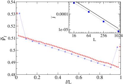
Figure 1: (Color online) ${\cal DC}$ density profile $\bar{\rho}_{l}$ across the ring for $f_{0}=0.3,f_{1}=0.2$, $\omega=0.2\pi$ and $\phi=\pi/2$ at half filling for two system sizes. Inset: ${\cal DC}$ current $\bar{J}\sim 1/L$ as shown by solid line of slope $-1$.

The model is defined on a ring with $L$ sites. A site $l=1,2...,L$ can be occupied by $n_{l}=0$ or $1$ particle, and the system contains a total of $N=\rho L$ particles where $\rho$ is the density. A particle at site $l$ hops to an empty site either on the left or right with rate $u_{l}=f_{0}$ for all $l\neq 1,L$ and $u_{1}=f_{0}+f_{1}\sin(\omega t),~{}u_{L}=f_{0}+f_{1}\sin(\omega t+\phi)$. For $f_{1}=0$, the above model reduces to the SEP with periodic boundary conditions, many of whose properties are known exactly Liggett (1985). The steady state obeys the equilibrium condition of detailed balance so that the current across a bond is zero. Due to this, the steady state measure is uniform and the $k$-point correlation function $C_{l_{1},l_{2},...,l_{k}}^{(0)}=\langle n_{l_{1}}n_{l_{2}}...n_{l_{k}}\rangle={L-k\choose N-k}/{L\choose N}$. As we will describe later, this knowledge of the exact steady state in the absence of time-dependent term in $u_{l}$ allows us to set up a perturbation expansion in $f_{1}$ of various observables.

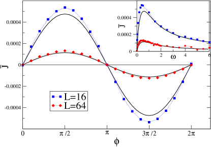
Figure 2: (Color online) Plot of $\bar{J}$ vs. $\phi$ with other parameters as in Fig. 1. The solid lines are from the perturbation theory.Inset shows plot of $\bar{J}$ vs. $\omega$

We first discuss the results of our Monte-Carlo simulations of the model defined above for generic values of the driving frequency $\omega$ and the phase $\phi$. We first look at the $\mathcal{DC}$ values of the current and local densities. In Fig. 1, we have plotted the local particle density profile for system sizes $L=16$ and $64$. We find a linear density profile in the bulk of the system with a discontinuity at the pumping sites. The linear density profile implies a $\mathcal{DC}$ current in the system. The inset in the figure shows that this current scales as $1/L$ as in driven SEP Derrida et al. (2002, 2004). In Fig. 2 we plot the current as a function of the applied phase difference for different system sizes. The prediction of the perturbation theory (described below) is also shown for comparison. As in the case of quantum pumps, we find a sinusoidal dependence of the current on the phase $\phi$. The inset of Fig. 2 shows the dependence of the current on the driving frequency $\omega$ again for $L=16,64$. At $\omega=0$, the system is in equilibrium and there is no current note1 . In the opposite limit $\omega\to\infty$, the system does not have time to react to the rapidly changing fields and we may again expect zero current. For any finite $\omega$, the ${\cal DC}$ current is nonzero and behaves as

$$\bar{J}\sim\begin{cases}\omega&\text{~{},~{}$\omega\ll\omega^{*}$,}\\ 1/\omega&\text{~{},~{} $\omega\gg\omega^{*}$}~{},\end{cases}$$ (1)

where $\omega^{*}$ is the frequency at which the current peaks. A similar non-monotonic behavior in current has been seen in experiments on ion pumps Astumian:2003 . Since $J\sim\omega$ as $\omega\to 0$, this means that a finite number of particles are circulated even in the adiabatic limit Astumian:2003 . This suggests a perturbation expansion in $\omega$ and will be discussed elsewhere. We also find that $\omega^{*}$ scales linearly with $f_{0}$, is independent of $L$ and hence of the typical relaxation time $\tau=L^{2}/f_{0}$ of the system.

Till now we have looked at various time averaged quantities. It is also of interest to look at the time dependences. In Fig. 3 we show the ensemble averaged local densities as a function of time obtained by an exact numerical integration of the $L=4,~{}N=2$ master equation. We find that the local densities oscillate about their respective ${\cal DC}$ value ( different from $\rho=0.5$) at large times, and a nonzero ${\cal DC}$ current circulates around the ring. Although the local ${\cal DC}$ density is close to $\rho$, the amplitude of the $\mathcal{AC}$ part is quite large. We also show a comparison of the exact density $\rho_{l}(t)$ with the approximate density $\rho+f_{1}\rho_{l}^{(1)}+f_{1}^{2}\rho_{l}^{(2)}$ obtained from the perturbation theory (see Eqs. (8) and (11)). We find that the ${\cal AC}$ density contains the driving frequency and also higher harmonics.

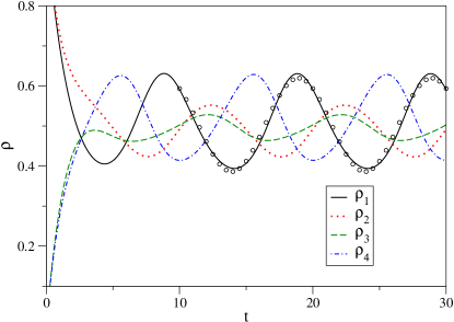
Figure 3: (Color online) Plot of time-dependent densities at the four sites of a $L=4$ lattice. In the initial configuration, sites $1$ and $2$ have one particle each and other sites are empty. The averages over one time period give: $\bar{\rho}_{1}=0.503493,~{}\bar{\rho}_{2}=0.498702,~{}\bar{\rho}_{3}=0.497417,~{}\bar{\rho}_{4}=0.500388$ and $\bar{J}=0.000514$. The points show the curve $\rho+f_{1}\rho_{1}^{(1)}+f_{1}^{2}\rho_{1}^{(2)}$. [Parameters: $f_{0}=0.4,~{}f_{1}=0.1,~{}\phi=\pi/2$ and $\omega=0.2\pi$].

We now proceed to describe a perturbation theory within which we will calculate an expression for the $\mathcal{DC}$ current $\bar{J}$ in the bulk of the system. Let us denote the site hopping rates by

$$u_{l}=f_{0}+f_{1}v_{l}=f_{0}+f_{1}(\nu_{l}e^{i\omega t}+\nu_{l}^{*}e^{-i\omega t})~{},$$ (2)

where the site-dependent complex amplitude $\nu_{1}=-i/2,\nu_{L}=-ie^{i\phi}/2$ and all other $\nu_{l}$’s are zero. We consider perturbative expansions of various quantities of interest with $f_{1}$ as the perturbation parameter about the homogeneous steady state corresponding to $f_{1}=0$. Thus we have

$$\rho_{l}(t) = \langle n_{l}(t)\rangle=\rho+\sum_{k=1}^{\infty}f_{1}^{k}\rho_{l}^{(k)}(t)$$

$$C_{l,m}(t) = \langle n_{l}(t)n_{m}(t)\rangle=C_{l,m}^{(0)}+\sum_{k=1}^{\infty}f_{1}^{k}C_{l,m}^{(k)}(t)~{},$$ (3)

and similar expressions for higher correlations. The current in a bond connecting sites $l$ and $l+1$ is given by $J_{l,l+1}(t)=u_{l}(\rho_{l}-C_{l,l+1})-u_{l+1}(\rho_{l+1}-C_{l,l+1})$ which can also be expanded in a perturbation series using Eq. (3). Averaging $J_{l,l+1}(t)$ over a time period for $\l\neq L-1,1,L$, we obtain constant ${\mathcal{D}C}$ current in the bulk note2 ,

$$\bar{J}=f_{0}\sum_{k=1}^{\infty}f_{1}^{k}\;(\bar{\rho}_{l}^{(k)}-\bar{\rho}_{l+1}^{(k)})$$ (4)

where $\bar{\rho}_{l}^{(k)}$ is the time-averaged density at the $k^{\rm th}$ order. To obtain $\bar{J}$ to leading order in $f_{1}$, we start with the exact equation of motion for the density $\rho_{l}$ Schütz (2000)

$$\frac{\partial\rho_{l}}{\partial t}+2u_{l}\rho_{l}-u_{l-1}\rho_{l-1}-u_{l+1}\rho_{l+1}$$ (5)

$$= u_{l}(C_{l-1,l}+C_{l,l+1})-u_{l+1}C_{l,l+1}-u_{l-1}C_{l-1,l}~{}.$$

Then the density $\rho_{l}^{(k)}$ at the $k^{\rm th}$ order evolves according to

$$\frac{\partial\rho_{l}^{(k)}}{\partial t}-{f_{0}}\Delta_{l}\rho_{l}^{(k)}+2v_{l}\rho_{l}^{(k-1)}-v_{l-1}\rho_{l-1}^{(k-1)}-v_{l+1}\rho_{l+1}^{(k-1)}$$ (6)

$$= v_{l}(C_{l-1,l}^{(k-1)}+C_{l,l+1}^{(k-1)})-v_{l-1}C_{l-1,l}^{(k-1)}-v_{l+1}C_{l,l+1}^{(k-1)}~{},$$

where $\Delta_{l}g_{l}=g_{l+1}-2g_{l}+g_{l-1}$ defines the discrete Laplacian operator. Thus, the density at the $k^{\rm th}$ order is obtainable in terms of the density and the two-point correlation function at $(k-1)^{\rm th}$ order.

At first order, the above equation simplifies to give

$$\frac{\partial\rho_{l}^{(1)}}{\partial t}-{f_{0}}\Delta_{l}\rho_{l}^{(1)}=r_{0}\Delta_{l}v_{l}~{},$$ (7)

where $r_{0}=\rho-C_{l_{1},l_{2}}^{(0)}$. In the steady state, integrating both sides of Eq. (7) over a time period, and using $\rho_{l}^{(1)}=\rho_{l+L}^{(1)}$ and density conservation, we find $\bar{\rho}_{l}^{(1)}=0$. Hence at ${\cal{O}}(f_{1})$, no $\cal{DC}$ current is generated. This is consistent with our expectation from linear response theory, namely that an $\cal{AC}$ field gives an $\cal{AC}$ response. Thus, we need to consider the next order term $\rho_{l}^{(2)}(t)$ in the perturbation expansion of the density to obtain current. As Eq. (6) for $k=2$ involves density at first order, we first solve for $\rho_{l}^{(1)}(t)$ in Eq. (7). The solution of this inhomogeneous linear equation is a sum of a homogeneous part which depends on initial conditions, and a particular integral. At long times, the homogeneous part can be shown to vanish (using the condition $\sum_{l}\rho_{l}^{(1)}(0)=0$) while the particular integral has the asymptotic form

$$\rho_{l}^{(1)}(t)=A_{l}^{(1)}e^{i\omega t}+A_{l}^{*(1)}e^{-i\omega t}$$ (8)

with the amplitudes given by

$$A_{l}^{(1)} = \alpha_{+}z_{+}^{l}+\alpha_{-}z_{-}^{l}~{}~{},~{}~{}l=2,3...,L-1$$

$$A_{1}^{(1)} = \alpha_{+}z_{+}+\alpha_{-}z_{-}-\frac{r_{0}\nu_{1}}{f_{0}}$$

$$A_{L}^{(1)} = \alpha_{+}z_{+}^{L}+\alpha_{-}z_{-}^{L}-\frac{r_{0}\nu_{L}}{f_{0}}~{}$$

where $z_{+}=y/2+[(y/2)^{2}-1]^{1/2},~{}z_{-}=1/z_{+},~{}y=2+i\omega/f_{0}$ and $\alpha_{\pm}=(-ir_{0}\omega/f_{0}^{2})(\nu_{1}z_{\mp}+\nu_{L})/[(z_{\pm}^{L}-1)(z_{\mp}-z_{\pm})]$. The amplitude of the density oscillations decay exponentially with distance from the pumping sites.

We also need the two-point correlation function $C_{l,m}^{(1)}$ at ${\cal O}(f_{1})$ appearing in Eq. (6) for $k=2$. Due to hard-core interaction, the correlation function $C_{l,m}$ for nearest neighbors $l$ and $m$ obeys a different equation of motion when $|l-m|\neq 1$. Taking care of this complication, it is straightforward to write down the corresponding evolution equations Schütz (2000) and carry out the perturbative expansion. At ${\cal O}(f_{1})$ in perturbation theory, we then get (for $1\leq l<L,~{}l+1<m\leq L$)

$$\frac{\partial C_{l,m}^{(1)}}{\partial t}-f_{0}(\Delta_{l}+\Delta_{m})C_{l,m}^{(1)}=k_{0}(\Delta_{l}v_{l}+\Delta_{m}v_{m})~{},$$

$$\frac{\partial C_{l,l+1}^{(1)}}{\partial t}+f_{0}\left(2C_{l,l+1}^{(1)}-C_{l-1,l+1}^{(1)}-C_{l,l+2}^{(1)}\right)$$

$$~{}~{}~{}~{}~{}~{}~{}~{}~{}~{}~{}~{}~{}~{}~{}~{}~{}~{}~{}~{}~{}~{}=k_{0}(v_{l-1}+v_{l+2}-v_{l}-v_{l+1})$$ (9)

where $k_{0}=C_{l_{1},l_{2}}^{(0)}-C_{l_{1},l_{2},l_{3}}^{(0)}$. The computation of even the homogenous solution of the above set of equations is in general a nontrivial task because of the form of the equations involving nearest neighbor indices and requires a Bethe ansatz or dynamic product ansatz Schütz (2000); Santos and Schütz (2001). However the long time solution can still be found exactly and is given by:

$$C_{l,m}^{(1)}(t)=\frac{k_{0}}{r_{0}}[\rho_{l}^{(1)}(t)+\rho_{m}^{(1)}(t)]=A_{l,m}^{(1)}e^{i\omega t}+A_{l,m}^{*(1)}e^{-i\omega t}~{},$$ (10)

where $A_{l,m}^{(1)}=(k_{0}/r_{0})(A_{l}^{(1)}+A_{m}^{(1)})$. It is easily verified that this satisfies Eq. (9) for all $l,m$. Interestingly, if one were to assume that the two-point function decouples, then a perturbation expansion to order $f_{1}$ will also yield the preceding equation in the thermodynamic limit. To determine whether the system indeed has a product measure requires a more detailed analysis of the higher order terms in the perturbation series and higher correlations, and will be discussed elsewhere.

We are now in a position to find the density profile $\rho_{l}^{(2)}(t)$. Using Eqs. (8) and (10) in Eq. (6) for $k=2$, we get

$$\rho_{l}^{(2)}(t)=\bar{\rho}_{l}^{(2)}+A_{l}^{(2)}e^{i2\omega t}+A_{l}^{*(2)}e^{-i2\omega t}$$ (11)

where the ${\cal DC}$ part $\bar{\rho}_{l}^{(2)}$ obeys the equation

$$f_{0}\Delta_{l}\bar{\rho}_{l}^{(2)}=2~{}{\rm Re}[2\nu_{l}^{*}A_{l}^{(1)}-\nu_{l-1}^{*}A_{l-1}^{(1)}-\nu_{l+1}^{*}A_{l+1}^{(1)}$$

$$-\nu_{l}^{*}(A_{l-1,l}^{(1)}+A_{l,l+1}^{(1)})+\nu_{l-1}^{*}A_{l-1,l}^{(1)}+\nu_{l+1}^{*}A_{l,l+1}^{(1)}]~{}.$$ (12)

Noting that the right hand side of the above equation is zero for most $l$, we get the following solution

$$\bar{\rho}_{l}^{(2)} = {s}l+h~{},~{}l=2,...,L-1$$

$$\bar{\rho}_{1}^{(2)} = {s}+h+\frac{2}{f_{0}}~{}{\rm Re}[\nu_{1}^{*}(A_{1,2}^{(1)}-A_{1}^{(1)})]$$

$$\bar{\rho}_{L}^{(2)} = {s}L+h+\frac{2}{f_{0}}~{}{\rm Re}[\nu_{L}^{*}(A_{L-1,L}^{(1)}-A_{L}^{(1)})]~{},$$ (13)

where the slope $s$ of the linear density profile is given by

$$s=\frac{2}{Lf_{0}}~{}{\rm Re}[\nu_{1}^{*}(A_{1,2}^{(1)}-A_{1,L}^{(1)})+\nu_{L}^{*}(A_{1,L}^{(1)}-A_{L-1,L}^{(1)})]~{},$$ (14)

and the intercept $h$ can be found using the particle conservation condition $\sum_{l}\rho_{l}^{(2)}=0$.

Our final result for the leading order contribution to the $\cal{DC}$ current in Eq. (4) is $\bar{J}=-f_{0}f_{1}^{2}s$ and, using the form of $A_{l,m}^{(1)}$, can be written as

$$\bar{J}=-\left(\frac{f_{1}}{f_{0}}\right)^{2}\frac{k_{0}\omega\sin\phi}{2L}~{}{\rm Re}\left(\frac{z_{+}-z_{+}^{L-1}}{1-z_{+}^{L}}\right)+{\cal O}(f_{1}^{3})~{}.$$ (15)

We observe that the $1/L$ dependence of the $\mathcal{DC}$ current and its sinusoidal variation with the phase are captured by the perturbation theory at ${\cal O}(f_{1}^{2})$. One can also check from the above expression that the frequency dependence of current in Eq. (1) is obtained with the typical frequency $\omega^{*}\approx 2f_{0},~{}L\gg 1$. As shown in Fig. (2) the above perturbative solution is already in a very good quantitative agreement with the simulation results.

To summarise, we have studied a stochastic model of hard-core particles on a ring in which periodically varying hopping rates can induce a $\cal{DC}$ current. A variation of our model defined on an open chain connected to particle reservoirs also shows nonzero $\cal{DC}$ current. Simulations and a novel perturbative analysis presented here show that many of the qualitative features are similar to that seen in quantum pumps. However unlike in quantum pumps, interactions play an essential role in our model. For non-interacting particles, noting that the bond current $J_{l,l+1}=u_{l}\rho_{l}-u_{l+1}\rho_{l+1}$ summed over all bonds is zero and using the uniformity of $\bar{J}$, it follows that no ${\cal DC}$ current is generated in this case. Our model can be generalised to include several pumps and pumps consisting of several sites, and these features could increase pumping efficiency.

K.J. thanks A. Rákos for useful discussions, Raman Research Institute for kind hospitality and Israel Science Foundation for financial support. A.D. thanks J.L.Lebowitz and E.R.Speer for useful discussions.

References

• Thouless (1983) D.ย J. Thouless, Phys. Rev. B 27, 6083 (1983).
• Switkes etย al. (1999) M.ย Switkes et ย al., Science 283, 1905 (1999); P.ย Leek et ย al., Phys.ย Rev.ย Lett.ย  95, 256802 (2005).
• Watson etย al. (2003) S.ย Watson et ย al., Phys. Rev. Lett. 91, 258301 (2003).
• (4) P.W. Brouwer, Phys. Rev. B 58, R10135 (1998); O.ย Entin-Wohlman, A.ย Aharony, and Y.ย Levinson, Phys. Rev. B 65, 195411 (2002); B.ย L. Altshuler and L.ย I. Glazman, Science 283, 1864 (1999). M.ย Strass; P.ย Hรคnggi, and S.ย Kohler, Phys.ย Rev.ย Lett.ย  95, 130601 (2005); A.ย Agarwal and D.ย Sen, J. Phys. Condens. Matter 19, 046205 (2007).
• Aleiner and Andreev (1998) I.ย Aleiner and A.ย Andreev, Phys. Rev. Lett. 81, 1286 (1998); P.ย Sharma and C.ย Chamon, Phys. Rev. Lett. 87, 096401 (2001); R.ย Citro, N.ย Andrei, and Q.ย Niu, Phys. Rev. B 68, 165312 (2003); E.ย Sela and Y.ย Oreg, Phys. Rev. Lett. 96, 166802 (2006).
• (6) M. Moskalets and M. Bรผttiker, Phys. Rev. B 64, 201305 (2001).
• (7) R.D.Astumian and I. Derenyi, Phys. Rev. Lett. 86, 3859 (2001)
• (8) R. Marathe, A.M.Jayannavar and A. Dhar, Phys. Rev. E 75, 030103(R) (2007).
• (9) N.A. Sinitsyn and I. Nemenman, Europhys. Lett. 77, 58001 (2007).
• (10) R. D. Astumian, Phys. Rev. Lett. 91, 118102 (2003).
• (11) R. D. Astumian and P. Hรคngii, Physics Today 55, 33 (2002).
• Reimann (2002) F.ย Jรผlicher, A.ย Ajdari, and J.ย Prost, Rev. Mod. Phys. 69, 1269 (1997); P.ย Reimann, Phys. Rep. 361, 57 (2002).
• Chou (1998) T.ย Chou, Phys. Rev. Lett. 80, 85 (1998).
• Wei etย al. (2000) Q.-H. Wei, C.ย Bechinger, and P.ย Leiderer, Science 287, 625 (2000).
• Liggett (1985) T.ย Liggett, Interacting particle systems (Springer-Verlag, New York, 1985).
• Spohn (1983) H.ย Spohn, J. Phys. A 16, 4275 (1983).
• Santos and Schรผtz (2001) J.E. Santos and G.M. Schรผtz, Phys. Rev. E 64, 036107 (2001).
• Derrida etย al. (2002) B.ย Derrida, J.ย L. Lebowitz, and E.ย R. Speer, J. Stat. Phys. 107, 599 (2002)
• Derrida etย al. (2004) B.ย Derrida, B.ย Douรงot, and P.-E. Roche, J. Stat. Phys. 115, 717 (2004).
• (20) R.D.Astumian and B.Robertson, J. Chem. Phys. 91, 4891 (1989).
• (21) In fact, one can verify that SEP with random, time-independent rates $w_{l}$ at site $l$ satisfies detailed balance with steady state measure $\sim\prod_{l=1}^{L}w_{l}^{-n_{l}}$.
• (22) That ${\cal DC}$ current $\bar{J}$ is same in all bonds follows on using that the density is conserved over a period in Eq.ย (5).
• Schรผtz (2000) G.M. Schรผtz, in Phase transitions and Critical Phenomena, edited by C.ย Domb and J.ย Lebowitz (Academic Press, London, 2000), pp. 3โ€“242.