Dynamical correlation functions of the XXZ model
at finite temperature

Abstract

Combining a lattice path integral formulation for thermodynamics with the solution of the quantum inverse scattering problem for local spin operators, we derive a multiple integral representation for the time-dependent longitudinal correlation function of the spin-1/2 Heisenberg XXZ chain at finite temperature and in an external magnetic field. Our formula reproduces the previous results in the following three limits: the static, the zero-temperature and the XY limits.

PACS numbers: 05.30.-d, 75.10.Pq, 02.30.Ik

1 Introduction

One of the most challenging problems in quantum many-body systems, especially in low-dimensions, is related to the evaluation of the correlation functions. Though many field theoretical schemes or numerical techniques have been developed and achieved remarkable success, the exact evaluation is in general still very difficult even in models which are exactly solvable by the Bethe ansatz methods.

The spin-1/2 Heisenberg XXZ chain is one of the simplest but non-trivial solvable models, and has served as a testing ground for many theoretical approaches. Concerning the correlation function of this model, Jimbo et al. [1, 2] derived a multiple integral representation of arbitrary correlators in the off-critical XXZ antiferromagnet at zero temperature and zero magnetic field. Their method utilizing the representation theory of the quantum affine algebra $U_{q}(\widehat{\mathfrak{sl}}_{2})$ has been extended to the XXX [3, 4], the massless XXZ [5] antiferromagnets.

Alternative approaches combining the algebraic Bethe ansatz and the solution of the quantum inverse scattering problem for local spin operators were proposed by Kitanine et al. in [6], and were applied to derive a multiple integral representation for both the critical and off-critical regimes of the XXZ model in finite magnetic field. Moreover they have obtained a new multiple integral representation which is more appropriate for the two-point correlators [7, 8], and have generalized further to the time-dependent longitudinal correlation function [9] (see [10] for a recent review). On the other hand, a finite temperature generalization was achieved more recently by Göhmann et al. by utilizing the quantum transfer matrix formalism for thermodynamics [11] (see also [12, 13, 14] for recent progress in this direction).

Motivated by these seminal works, in this paper, we generalize the result [9, 11] to the time-dependent longitudinal correlation function at finite temperature. By combining a lattice path integral formulation with the solution of the quantum inverse scattering problem, we derive a multiple integral representing a generating function of the time-dependent correlation function for the $z$-components of the spins. In the zero-temperature, the static and the XY limits, our formula reproduces the results in [9, 11, 15].

The layout of this paper is as follows. In the subsequent section we introduce the spin-1/2 Heisenberg XXZ chain and its classical counterpart. Utilizing a lattice path integral formulation together with the solution of the quantum inverse scattering problem for local spins, in Section 3, we formulate the generating function characterizing the time-dependent longitudinal correlation function at finite temperature. In Section 4, we derive a multiple integral representing the generating function by combining the method developed in [7, 9] and [11]. The following three limits, namely the static, the zero-temperature and the XY limits are considered in Section 5. Section 6 is devoted to a brief conclusion.

2 Spin-1/2 Heisenberg XXZ chain

The Hamiltonian of the spin-1/2 Heisenberg XXZ chain defined on a periodic lattice of length $L$ is given by

$$\mathscr{H}=\mathscr{H}_{0}-hS^{z},$$ (2.1)

where

$$\mathscr{H}_{0}=J\sum_{j=1}^{L}\left\{\sigma_{j}^{x}\sigma_{j+1}^{x}+\sigma_{j}^{y}\sigma_{j+1}^{y}+\Delta(\sigma_{j}^{z}\sigma_{j+1}^{z}-1)\right\},\quad S^{z}=\frac{1}{2}\sum_{j=1}^{L}\sigma_{j}^{z}.$$ (2.2)

Here $\sigma_{j}^{x,y,z}$ are the Pauli matrices acting on the two-dimensional quantum space $\mathcal{H}_{j}$ at site $j$. The real parameter $\Delta_{\geq 0}$ is the anisotropy parameter, and $J\in\mathbb{R}$ fixes the energy scale of the model. In this paper, we consider the model at finite temperature $T\geq 0$ and in a finite magnetic filed $h\in\mathbb{R}$.

It is well-known that a $d$-dimensional quantum system can be mapped onto a $(d+1)$-dimensional classical system. The classical counterpart of the XXZ model is so-called the six-vertex model whose Boltzmann weights can be described as the elements of the $\mathscr{R}$-matrix $\mathscr{R}(\lambda)\in{\rm End}(\mathbb{C}^{2}\otimes\mathbb{C}^{2})$,

$$\mathscr{R}(\lambda)=\begin{pmatrix}1&0&0&0\\ 0&\frac{\operatorname{sh}\lambda}{\operatorname{sh}(\lambda+\eta)}&\frac{\operatorname{sh}\eta}{\operatorname{sh}(\lambda+\eta)}&0\\ 0&\frac{\operatorname{sh}\eta}{\operatorname{sh}(\lambda+\eta)}&\frac{\operatorname{sh}\lambda}{\operatorname{sh}(\lambda+\eta)}&0\\ 0&0&0&1\end{pmatrix}.$$ (2.3)

Identifying one of the two vector spaces of the above $\mathscr{R}$-matrix with the quantum space $\mathcal{H}_{j}$, we define the monodromy matrix $\mathscr{T}^{\rm R}_{\bar{i}}(\lambda)$ as

$$\mathscr{T}^{\rm R}_{{\bar{i}}}(\lambda)=\mathscr{R}_{{\bar{i}}L}(\lambda)\cdots\mathscr{R}_{{\bar{i}}2}(\lambda)\mathscr{R}_{{\bar{i}}1}(\lambda),$$ (2.4)

where $\mathscr{R}_{{\bar{i}}j}(\lambda)$ acts in the space $\mathcal{H}_{\bar{i}}\otimes\mathcal{H}_{j}$ (see also figure 1 for a graphical representation of $\mathscr{R}_{{\bar{i}}j}(\lambda)$ and $\mathscr{T}^{\rm R}_{{\bar{i}}}(\lambda)$). Since the $\mathscr{R}$-matrix satisfies the Yang-Baxter equation

$$\mathscr{R}_{12}(\lambda-\mu)\mathscr{R}_{13}(\lambda-\nu)\mathscr{R}_{23}(\mu-\nu)=\mathscr{R}_{23}(\mu-\nu)\mathscr{R}_{13}(\lambda-\nu)\mathscr{R}_{12}(\lambda-\mu),$$ (2.5)

the transfer matrix defined by $T_{\rm R}(\lambda)=\operatorname{Tr}_{{\bar{i}}}\mathscr{T}^{\rm R}_{{\bar{i}}}(\lambda)$ commutes for different spectral parameters: $[T_{\rm R}(\lambda),T_{\rm R}(\mu)]=0$. Using the following relation connecting the six-vertex model with the XXZ model (2.1):

$$\mathscr{H}_{0}=2J\operatorname{sh}(\eta)T^{-1}_{\rm R}(0)T_{\rm R}^{\prime}(0),\qquad\Delta=\operatorname{ch}\eta,$$ (2.6)

one can expand the transfer matrix with respect to the spectral parameter $\lambda$

$$T_{\rm R}(\lambda)=T_{\rm R}(0)\left(1+\frac{\lambda}{2J\operatorname{sh}\eta}\mathscr{H}_{0}+\mathcal{O}(\lambda^{2})\right).$$ (2.7)

For later convenience, let us introduce another type of transfer matrix defined by

$${\overline{T}}_{\rm R}(\lambda)=\operatorname{Tr}_{{\bar{i}}}\left[\mathscr{R}_{L{\bar{i}}}(-\lambda)\cdots\mathscr{R}_{2{\bar{i}}}(-\lambda)\mathscr{R}_{1{\bar{i}}}(-\lambda)\right].$$ (2.8)

Note that $T_{\rm R}(0)$ and ${\overline{T}}_{\rm R}(0)$ are respectively the right- and left-shift operators, and hence

$${\overline{T}}_{\rm R}(0)=T_{\rm R}^{-1}(0).$$ (2.9)

Using this together with the expansion (2.7), one arrives at a crucial formula

$$\lim_{N\to\infty}\left[{\overline{T}}_{\rm R}(\lambda)T_{\rm R}\left(\lambda+\frac{\beta}{N}\right)\right]^{\frac{N}{2}}\Biggr{|}_{\lambda=0}=\exp\left(\frac{\beta}{4J\operatorname{sh}\eta}\mathscr{H}_{0}\right),\quad\beta\in\mathbb{C},$$ (2.10)

where $N\in 2\mathbb{N}$ is assumed.

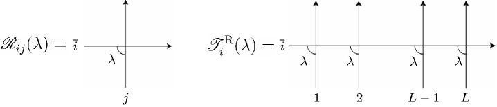
Figure 1: A graphical representation for the $\mathscr{R}$-matrix $\mathscr{R}(\lambda)$ (2.3) and the monodromy matrix $\mathscr{T}_{\bar{i}}(\lambda)$ (2.4).

3 Time-dependent generating function at finite temperature

3.1 Quantum transfer matrix

Our main aim in this paper is to derive a multiple integral representation of the time-dependent longitudinal correlation function $\langle\sigma_{1}^{z}(0)\sigma_{m+1}^{z}(t)\rangle$ for the XXZ model (2.1) at finite temperature. To this end, we firstly consider how the time-dependent correlator is described by the transfer matrix formalism.

Since $[S^{z},\sigma_{j}^{z}]=0$, the time-dependent local spin operator $\sigma_{j}^{z}(t)$ can be written as

$$\sigma^{z}_{j}(t)={\rm e}^{{\rm i}\mathscr{H}_{0}t}\sigma_{j}^{z}{\rm e}^{-{\rm i}\mathscr{H}_{0}t}.$$ (3.1)

Using this and noticing that $[\mathscr{H}_{0},S^{z}]=0$, one immediately sees

$$\langle\sigma_{1}^{z}(0)\sigma_{m+1}^{z}(t)\rangle=\frac{\operatorname{Tr}\left\{{\rm e}^{-\mathscr{H}/T}{\rm e}^{-{\rm i}\mathscr{H}_{0}t}\sigma_{1}^{z}{\rm e}^{{\rm i}\mathscr{H}_{0}t}\sigma_{m+1}^{z}\right\}}{\operatorname{Tr}{\rm e}^{-\mathscr{H}/T}}.$$ (3.2)

Here we have set the Boltzmann constant to unity. Applying the formula (2.10), we insert the relations

$${\rm e}^{-\mathscr{H}/T}=\lim_{N_{0}\to\infty}{\rm e}^{\frac{hS^{z}}{T}}\left\{{\overline{T}}_{\rm R}(\lambda)T_{\rm R}(\lambda-\varepsilon_{0})\right\}^{\frac{N_{0}}{2}}\Bigg{|}_{\lambda=0}, \qquad\varepsilon_{0}=\frac{\beta_{0}}{N_{0}},\quad\beta_{0}=\frac{4J\operatorname{sh}\eta}{T},$$

$${\rm e}^{\pm{\rm i}\mathscr{H}_{0}t}=\lim_{N_{1}\to\infty}\left\{{\overline{T}}_{\rm R}(\lambda)T_{\rm R}(\lambda\pm\varepsilon_{1})\right\}^{\frac{N_{1}}{2}}\Bigg{|}_{\lambda=0}, \qquad\varepsilon_{1}=\frac{\beta_{1}}{N_{1}},\quad\beta_{1}=4{\rm i}tJ\operatorname{sh}\eta,$$ (3.3)

into (3.2). The result can be graphically represented as in figure 2.

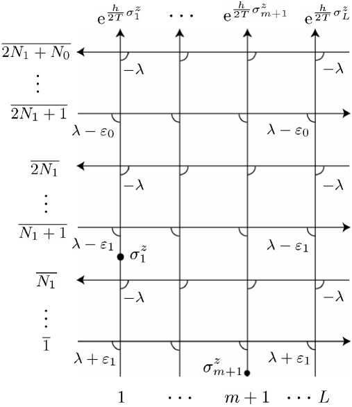
Figure 2: A graphical representation for the longitudinal dynamical correlation function $\langle\sigma_{1}^{z}(0)\sigma_{m+1}^{z}(t)\rangle$. Here $\varepsilon_{0}=\beta_{0}/N_{0}$ and $\varepsilon_{1}=\beta_{1}/N_{1}$. We assume the lattice is on a torus. The correlation function (multiplied by the partition function $\operatorname{Tr}{\rm e}^{-\mathscr{H}/T}$) is reproduced by setting $\lambda=0$ and taking the limit $N_{0,1}\to\infty$. The partition function $\operatorname{Tr}{\rm e}^{-\mathscr{H}/T}$ is obtained by just replacing $\sigma_{1}^{z}$ and $\sigma_{m+1}^{z}$ with the identity operator.

As proved in [16, 17, 18], the local spin operator $\sigma_{j}^{z}$ is expressed in terms of the transfer matrix:

$$\sigma_{j}^{z}=T_{\rm R}^{j-1}(0)\operatorname{Tr}_{{\bar{i}}}[\sigma_{{\bar{i}}}^{z}\mathscr{T}^{\rm R}_{{\bar{i}}}(0)]T_{\rm R}^{-j}(0).$$ (3.4)

Thus, substituting

$$\sigma^{z}_{1}=\lim_{\varepsilon\to 0}\operatorname{Tr}_{{\bar{i}}}[\sigma_{{\bar{i}}}^{z}\mathscr{T}^{\rm R}_{{\bar{i}}}(\lambda-\varepsilon)]{\overline{T}}_{\rm R}(\lambda)\Bigr{|}_{\lambda=0},\quad\varepsilon\in\mathbb{C}$$ (3.5)

which is obtained by (3.4) and (2.9), one finds $\langle\sigma_{1}^{z}(0)\sigma_{m+1}^{z}(t)\rangle$ is given by a product of the transfer matrix and two local operators located on the boundaries (see figure 3).

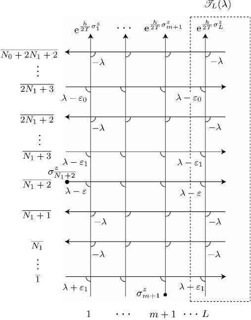
Figure 3: A graphical representation of the quantum transfer matrix $T(\lambda)=\operatorname{Tr}_{j}\mathscr{T}_{j}(\lambda)$ (surrounded by broken lines). In fact, a small parameter $\varepsilon$ is introduced to avoid that the quantum transfer matrix becomes a singular matrix. The partition function $\operatorname{Tr}{\rm e}^{-\mathscr{H}/T}$ is obtained by replacing $\sigma_{m+1}^{z}$ and $\sigma_{\overline{N_{1}+2}}^{z}$ with the identity operator.

To consider the system at finite temperature, let us introduce the quantum transfer matrix $T(\lambda)$ acting in the space $\otimes_{{\bar{i}}=1}^{\overline{N_{0}+2N_{1}+2}}\mathcal{H}_{{\bar{i}}}$:

$$T(\lambda)=\operatorname{Tr}_{j}\mathscr{T}_{j}(\lambda).$$ (3.6)

Here $\mathscr{T}_{j}(\lambda)$ is defined by

$$\mathscr{T}_{j}(\lambda)= {\rm e}^{\frac{h}{2T}\sigma_{j}^{z}}\mathscr{R}_{j\overline{N_{0}+2N_{1}+2}}(-\lambda)\mathscr{R}_{\overline{N_{0}+2N_{1}+1}j}(\lambda-\varepsilon_{0})\cdots\mathscr{R}_{j\overline{2N_{1}+4}}(-\lambda)\mathscr{R}_{\overline{2N_{1}+3}j}(\lambda-\varepsilon_{0})$$

$$\times\mathscr{R}_{j\overline{2N_{1}+2}}(-\lambda)\mathscr{R}_{\overline{2N_{1}+1}j}(\lambda-\varepsilon_{1})\cdots\mathscr{R}_{j\overline{N_{1}+4}}(-\lambda)\mathscr{R}_{\overline{N_{1}+3}j}(\lambda-\varepsilon_{1})$$

$$\times\mathscr{R}_{\overline{N_{1}+2}j}(\lambda-\varepsilon)\mathscr{R}_{j\overline{N_{1}+1}}(-\lambda)$$

$$\times\mathscr{R}_{j\overline{N_{1}}}(-\lambda)\mathscr{R}_{\overline{N_{1}-1}j}(\lambda+\varepsilon_{1})\cdots\mathscr{R}_{j\overline{2}}(-\lambda)\mathscr{R}_{\overline{1}j}(\lambda+\varepsilon_{1}).$$ (3.7)

In figure 3, we also schematically depict the quantum transfer matrix. Thanks to the Yang-Baxter equation (2.5), we see the quantum transfer matrix commutes for different spectral parameters: $[T(\lambda),T(\mu)]=0.$ Thus the dynamical correlation function (3.2) is expressed in terms of $T(\lambda)$:

$$\langle\sigma_{1}^{z}(0)\sigma_{m+1}^{z}(t)\rangle=\lim_{N_{0},N_{1}\to\infty}\lim_{\varepsilon\to 0}\frac{\operatorname{Tr}_{1,\dots,L}\left[T^{L-m-1}(\varepsilon)(A-D)(\varepsilon)T^{m}(\varepsilon)\sigma_{\overline{N_{1}+2}}^{z}\right]}{\operatorname{Tr}_{1,\dots,L}T^{L}(\varepsilon)},$$ (3.8)

where $A(\lambda)$ and $D(\lambda)$ are elements of the monodromy matrix $\mathscr{T}(\lambda)$ represented as a $2\times 2$ matrix

$$\mathscr{T}(\lambda)=\left(\begin{array}[]{@{\,}cc@{\,}}A(\lambda)&B(\lambda)\\ C(\lambda)&D(\lambda)\end{array}\right)$$ (3.9)

in the quantum space. In this definition, $T(\lambda)$ is given by $T(\lambda)=A(\lambda)+D(\lambda)$.

Let us consider the thermodynamic limit $L\to\infty$. Since the limits $L\to\infty$ and $N_{0},N_{1}\to\infty$ are interchangeable as proved in [19, 20], one can take the limit $L\to\infty$ first. In addition, we find the leading eigenvalue of the quantum transfer matrix $T(0)$ (written as $\Lambda_{0}(0)$) is non-degenerate and separated from the next-leading eigenvalues by a finite gap even in the Trotter limit $N_{0},N_{1}\to\infty$. In the thermodynamic limit $L\to\infty$, therefore, (3.8) is characterized by $\Lambda_{0}(0)$ and the corresponding (normalized) eigenstate $|\Psi\rangle$:

$$\langle\sigma_{1}^{z}(0)\sigma_{m+1}^{z}(t)\rangle=\lim_{N_{0},N_{1}\to\infty}\lim_{\varepsilon\to 0}\Lambda^{-m-1}_{0}(\varepsilon)\langle\Psi|(A-D)(\varepsilon)T^{m}(\varepsilon)\sigma_{\overline{N_{1}+2}}^{z}|\Psi\rangle.$$ (3.10)

Inserting the relation

$$\sigma_{\overline{N_{1}+2}}^{z}= \left[T(-\varepsilon_{1})T^{-1}(0)\right]^{\frac{N_{1}}{2}}T^{-1}(0)(A-D)(\varepsilon)T^{-1}(\varepsilon)T(0)\left[T(0)T^{-1}(-\varepsilon_{1})\right]^{\frac{N_{1}}{2}},$$ (3.11)

which is a ‘quantum transfer matrix analogue’ of (3.4), we finally obtain

$$\langle\sigma_{1}^{z}(0)\sigma_{m+1}^{z}(t)\rangle=\lim_{N_{0},N_{1}\to\infty}\lim_{\varepsilon\to 0}\langle\Psi| (A-D)(\varepsilon)T^{m-1}(\varepsilon)Q$$

$$\times(A-D)(\varepsilon)Q^{-1}T^{-m-1}(\varepsilon)|\Psi\rangle,$$ (3.12)

where $Q=T(\varepsilon)T^{-1}(0)\left[T^{-1}(0)T(-\varepsilon_{1})\right]^{\frac{N_{1}}{2}}.$

3.2 Generating function for dynamical correlation function

It is convenient to introduce the following operator as in [9]:

$$\mathscr{Q}^{\kappa}_{l+1,m}=T^{l}(\varepsilon)T_{\kappa}^{m-l}(\varepsilon)Q_{\kappa}T^{-m}(\varepsilon)Q^{-1}.$$ (3.13)

Here $T_{\kappa}(\lambda)$ and $Q_{\kappa}$ are respectively defined by

$$T_{\kappa}(\lambda)=A(\lambda)+\kappa D(\lambda),\quad Q_{\kappa}=T_{\kappa}(\varepsilon)T^{-1}_{\kappa}(0)\left[T^{-1}_{\kappa}(0)T_{\kappa}(-\varepsilon_{1})\right]^{\frac{N_{1}}{2}}.$$ (3.14)

Due to the Yang-Baxter equation (2.5), the twisted quantum transfer matrix $T_{\kappa}(\lambda)$ is commutative as long as the twist angle $\kappa$ is taken the same: $[T_{\kappa}(\lambda),T_{\kappa}(\mu)]=0.$ It follows that

$$\left\langle\frac{1-\sigma_{l+1}^{z}(0)}{2}\frac{1-\sigma_{m+1}^{z}(t)}{2}\right\rangle =\lim_{N_{0},N_{1}\to\infty}\lim_{\varepsilon\to 0}\langle\Psi|T^{l}(\varepsilon)D(\varepsilon)T^{m-l-1}(\varepsilon)Q$$

$$\qquad\qquad\qquad\qquad\qquad\times D(\varepsilon)Q^{-1}T^{-m-1}(\varepsilon)|\Psi\rangle$$

$$=\lim_{N_{0},N_{1}\to\infty}\lim_{\varepsilon\to 0}\frac{1}{2}\partial_{\kappa}^{2}\langle\Psi|\mathscr{Q}^{\kappa}_{l+1,m+1}-\mathscr{Q}_{l+2,m+1}^{\kappa}-\mathscr{Q}_{l+1,m}^{\kappa}+\mathscr{Q}^{\kappa}_{l+2,m}|\Psi\rangle\bigl{|}_{\kappa=1}.$$ (3.15)

Because of the translational invariance for the correlation functions, one can set $l=0$ without loss of generality. Introducing the generating function

$$\mathcal{Q}_{\kappa}(m,t)=\lim_{N_{0},N_{1}\to\infty}\lim_{\varepsilon\to 0}\langle\Psi|\mathscr{Q}^{\kappa}_{1,m}|\Psi\rangle,$$ (3.16)

one obtains the longitudinal time-dependent correlation function (3.2):

$$\langle\sigma_{1}^{z}(0)\sigma_{m+1}^{z}(t)\rangle=2D_{m}^{2}\partial_{\kappa}^{2}\mathcal{Q}_{\kappa}(m,t)\bigl{|}_{\kappa=1}+2\langle\sigma^{z}\rangle-1,$$ (3.17)

where $\langle\sigma^{z}\rangle$ is the magnetization (multiplied by a factor 2) and $D_{m}$ denotes the lattice derivative defined by

$$D_{m}g(m)=g(m+1)-g(m),\quad D^{2}_{m}g(m)=g(m+1)-2g(m)+g(m-1),\quad m\in\mathbb{N}.$$ (3.18)

3.3 Bethe ansatz

To evaluate (3.16) actually, we need to investigate the leading eigenvalue and the corresponding eigenstate. Here we derive a general formula describing the eigenvalues and the corresponding eigenstates through the solutions to a certain algebraic equation called the Bethe ansatz equation.

Let us define the ‘vacuum state’ $|0\rangle$ as

$$|0\rangle:= \underbrace{\binom{1}{0}_{\overline{1}}\otimes\binom{0}{1}_{\overline{2}}\otimes\cdots\otimes\binom{0}{1}_{\overline{N_{1}}}}_{N_{1}{\rm\,factors}}\otimes\binom{0}{1}_{\overline{N_{1}+1}}\otimes\binom{1}{0}_{\overline{N_{1}+2}}$$

$$\underbrace{\otimes\binom{1}{0}_{\overline{N_{1}+3}}\otimes\binom{0}{1}_{\overline{N_{1}+4}}\otimes\cdots\otimes\binom{0}{1}_{\overline{2N_{1}+2}}}_{N_{1}{\rm\,factors}}$$

$$\underbrace{\otimes\binom{1}{0}_{\overline{2N_{1}+3}}\otimes\binom{0}{1}_{\overline{2N_{1}+4}}\otimes\cdots\otimes\binom{0}{1}_{\overline{N_{0}+2N_{1}+2}}}_{N_{0}{\rm\,factors}}.$$ (3.19)

Obviously (3.19) is an eigenstate of the (twisted) quantum transfer matrix $T_{\kappa}(\lambda)$. Explicitly

$$T_{\kappa}(\lambda)|0\rangle=(a(\lambda)+\kappa d(\lambda))|0\rangle,\quad A(\lambda)|0\rangle=a(\lambda)|0\rangle,\quad D(\lambda)|0\rangle=d(\lambda)|0\rangle,$$ (3.20)

where

$$a(\lambda) =\left\{\frac{\operatorname{sh}\lambda}{\operatorname{sh}(\lambda-\eta)}\right\}^{\frac{N_{0}}{2}+N_{1}+1}{\rm e}^{\frac{h}{2T}},$$

$$d(\lambda) =\left\{\frac{\operatorname{sh}(\lambda+\varepsilon_{1})}{\operatorname{sh}(\lambda+\varepsilon_{1}+\eta)}\frac{\operatorname{sh}(\lambda-\varepsilon_{1})}{\operatorname{sh}(\lambda-\varepsilon_{1}+\eta)}\right\}^{\frac{N_{1}}{2}}\left\{\frac{\operatorname{sh}(\lambda-\varepsilon_{0})}{\operatorname{sh}(\lambda-\varepsilon_{0}+\eta)}\right\}^{\frac{N_{0}}{2}}\frac{\operatorname{sh}(\lambda-\varepsilon)}{\operatorname{sh}(\lambda-\varepsilon+\eta)}{\rm e}^{-\frac{h}{2T}}.$$ (3.21)

In the framework of the algebraic Bethe ansatz, the vector $|\{\lambda\}_{\kappa}\rangle$ constructed by the multiple action of $B(\lambda)$, namely $|\{\lambda^{\kappa}\}\rangle=\prod_{j=1}^{M}B(\lambda^{\kappa}_{j})|0\rangle$, is an eigenstate of $T_{\kappa}(\lambda)$ if the rapidities $\{\lambda_{j}^{\kappa}\}_{j=1}^{M}$ satisfy the following Bethe ansatz equation:

$$\frac{a(\lambda_{j}^{\kappa})}{d(\lambda_{j}^{\kappa})}=-\kappa\prod_{k=1}^{M}\frac{\operatorname{sh}(\lambda^{\kappa}_{j}-\lambda^{\kappa}_{k}+\eta)}{\operatorname{sh}(\lambda^{\kappa}_{j}-\lambda^{\kappa}_{k}-\eta)}.$$ (3.22)

The corresponding eigenvalue is given by

$$\Lambda(\lambda,\kappa)=a(\lambda)\prod_{j=1}^{M}\frac{\operatorname{sh}(\lambda-\lambda_{j}^{\kappa}-\eta)}{\operatorname{sh}(\lambda-\lambda_{j}^{\kappa})}+\kappa d(\lambda)\prod_{j=1}^{M}\frac{\operatorname{sh}(\lambda-\lambda_{j}^{\kappa}+\eta)}{\operatorname{sh}(\lambda-\lambda_{j}^{\kappa})}.$$ (3.23)

Hereafter we restrict ourselves on the case $\kappa=1$ in (3.22) and simply write the roots and the eigenstate corresponding to the leading eigenvalue $\Lambda_{0}(0)(=\Lambda_{0}(0,1))$ as $\{\lambda_{j}\}_{j=1}^{N/2}$ ($N=N_{0}+2N_{1}+2$) and $|\{\lambda\}\rangle$, respectively. To make the analysis possible even in the Trotter limit $N\to\infty$, we utilize a powerful method as in [21, 22, 23]. Let us consider the following auxiliary function

$${\mathfrak{a}}(\lambda)=\frac{d(\lambda)}{a(\lambda)}\prod_{k=1}^{\frac{N}{2}}\frac{\operatorname{sh}(\lambda-\lambda_{k}+\eta)}{\operatorname{sh}(\lambda-\lambda_{k}-\eta)},\quad N=N_{0}+2N_{1}+2,$$ (3.24)

which associates the Bethe ansatz roots $\{\lambda_{j}\}_{j=1}^{N/2}$ with zeros of $1+{\mathfrak{a}}(\lambda)$. By studying the analyticity properties of the auxiliary function, one sees ${\mathfrak{a}}(\lambda)$ satisfies the following nonlinear integral equation:

$$\ln{\mathfrak{a}}(\lambda)= -\frac{h}{T}+\ln\frac{\operatorname{sh}(\lambda+\eta)\operatorname{sh}(\lambda-\varepsilon)}{\operatorname{sh}(\lambda)\operatorname{sh}(\lambda-\varepsilon+\eta)}+\frac{N_{0}}{2}\ln\frac{\operatorname{sh}(\lambda+\eta)\operatorname{sh}(\lambda-\varepsilon_{0})}{\operatorname{sh}(\lambda)\operatorname{sh}(\lambda-\varepsilon_{0}+\eta)}$$

$$+\frac{N_{1}}{2}\ln\frac{\operatorname{sh}(\lambda+\eta)\operatorname{sh}(\lambda+\varepsilon_{1})}{\operatorname{sh}(\lambda)\operatorname{sh}(\lambda+\varepsilon_{1}+\eta)}+\frac{N_{1}}{2}\ln\frac{\operatorname{sh}(\lambda+\eta)\operatorname{sh}(\lambda-\varepsilon_{1})}{\operatorname{sh}(\lambda)\operatorname{sh}(\lambda-\varepsilon_{1}+\eta)}$$

$$-\int_{\mathcal{C}}\frac{{\rm d}\omega}{2\pi{\rm i}}\frac{\operatorname{sh}(2\eta)\ln(1+{\mathfrak{a}}(\omega))}{\operatorname{sh}(\lambda-\omega+\eta)\operatorname{sh}(\lambda-\omega-\eta)}.$$ (3.25)

Here the contour $\mathcal{C}$ is taken, for instance, as a rectangular contour whose edges are parallel to the real axis at $\pm\pi{\rm i}/2$ (respectively $\pm\eta/2$) and are parallel to the imaginary axis at $\pm\eta/2$ (respectively $\pm\infty$) for the off-critical regime $\Delta=\operatorname{ch}\eta>1$ (respectively for the critical regime $0\leq\Delta=\operatorname{ch}\eta\leq 1$) (see figure 4 for a pictorial definition). In (3.25) the limits $N_{0},N_{1}\to\infty$ and $\varepsilon\to 0$ can be taken analytically. We thus obtain

$$\ln{\mathfrak{a}}(\lambda)=-\frac{h}{T}-\frac{2J\operatorname{sh}^{2}(\eta)}{T\operatorname{sh}(\lambda)\operatorname{sh}(\lambda+\eta)}-\int_{\mathcal{C}}\frac{{\rm d}\omega}{2\pi{\rm i}}\frac{\operatorname{sh}(2\eta)\ln(1+{\mathfrak{a}}(\omega))}{\operatorname{sh}(\lambda-\omega+\eta)\operatorname{sh}(\lambda-\omega-\eta)},$$ (3.26)

which is exactly the same as that in [11]. For later convenience, here we also introduce another auxiliary function $\overline{{\mathfrak{a}}}(\lambda)=1/{\mathfrak{a}}(\lambda)$ satisfying the following nonlinear integral equation in the limits $N_{0},N_{1}\to\infty$ and $\varepsilon\to 0$ [11]:

$$\ln\overline{{\mathfrak{a}}}(\lambda)=\frac{h}{T}-\frac{2J\operatorname{sh}^{2}(\eta)}{T\operatorname{sh}(\lambda)\operatorname{sh}(\lambda-\eta)}+\int_{\mathcal{C}}\frac{{\rm d}\omega}{2\pi{\rm i}}\frac{\operatorname{sh}(2\eta)\ln(1+\overline{{\mathfrak{a}}}(\omega))}{\operatorname{sh}(\lambda-\omega+\eta)\operatorname{sh}(\lambda-\omega-\eta)}.$$ (3.27)

By this auxiliary function ${\mathfrak{a}}(\lambda)$, the leading eigenvalue of the quantum transfer matrix related to the free energy density $f$ by $f=-T\ln\Lambda_{0}(0)$ is expressed as a single integral form

$$\ln\Lambda_{0}(0)=\frac{h}{2T}+\int_{\mathcal{C}}\frac{{\rm d}\omega}{2\pi{\rm i}}\frac{\operatorname{sh}(\eta)\ln(1+{\mathfrak{a}}(\omega))}{\operatorname{sh}(\omega)\operatorname{sh}(\omega+\eta)}=-\frac{h}{2T}-\int_{\mathcal{C}}\frac{{\rm d}\omega}{2\pi{\rm i}}\frac{\operatorname{sh}(\eta)\ln(1+\overline{{\mathfrak{a}}}(\omega))}{\operatorname{sh}(\omega)\operatorname{sh}(\omega-\eta)}.$$ (3.28)

Differentiating (3.28) with respect to $h$, one has the magnetization (multiplied by a factor 2),

$$\langle\sigma^{z}\rangle=1+T\int_{\mathcal{C}}\frac{{\rm d}\omega}{\pi{\rm i}}\frac{\operatorname{sh}(\eta)\partial_{h}{\mathfrak{a}}(\omega)}{\operatorname{sh}(\omega)\operatorname{sh}(\omega+\eta)(1+{\mathfrak{a}}(\omega))}=-1-T\int_{\mathcal{C}}\frac{{\rm d}\omega}{\pi{\rm i}}\frac{\operatorname{sh}(\eta)\partial_{h}\overline{{\mathfrak{a}}}(\omega)}{\operatorname{sh}(\omega)\operatorname{sh}(\omega-\eta)(1+\overline{{\mathfrak{a}}}(\omega))}.$$ (3.29)

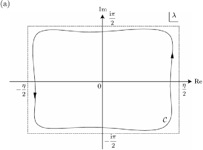
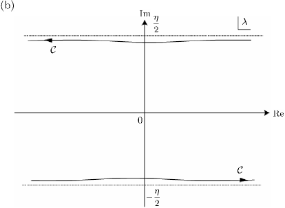
Figure 4: The integration contours for the off-critical regime $\Delta>1$ (a) and for the critical regime $0\leq\Delta\leq 1$ (b).

4 Multiple integral representation

In this section, using the method developed in [11], we derive a multiple integral representation of the longitudinal dynamical correlation function $\langle\sigma_{1}^{z}(0)\sigma_{m+1}^{z}(t)\rangle$ at finite temperature. Utilizing the relation $T_{\kappa}(0)T_{\kappa}(\eta)=\kappa a(\eta)d(0),$ which can easily be obtained from (3.23), one expresses the operator $\mathscr{Q}_{1,m}^{\kappa}$ (3.13) as

$$\mathscr{Q}_{1,m}^{\kappa}=\kappa^{-\frac{N_{1}}{2}-1} [T_{\kappa}^{m+1}(\varepsilon)T_{\kappa}^{\frac{N_{1}}{2}}(-\varepsilon_{1})]T_{\kappa}^{\frac{N_{1}}{2}+1}(\eta)[T^{-m-1}(\varepsilon)T^{-\frac{N_{1}}{2}}(-\varepsilon_{1})]T^{-\frac{N_{1}}{2}-1}(\eta).$$ (4.1)

To analyze the above quantity, we conveniently introduce a set of parameters $\xi_{1},\dots,\xi_{{\widehat{m}}+{\widetilde{m}}}$ (${\widehat{m}}=N_{1}/2+m+1$, ${\widetilde{m}}=N_{1}/2+1$) located inside $\mathcal{C}$ and define

$$(x_{1},\dots,x_{{\widehat{m}}+{\widetilde{m}}}) =({\widehat{x}}_{1},\dots,{\widehat{x}}_{{\widehat{m}}};{\widetilde{x}}_{1},\dots,{\widetilde{x}}_{{\widetilde{m}}})$$

$$=(\xi_{1}+\varepsilon,\dots,\xi_{m+1}+\varepsilon,\xi_{m+2}-\varepsilon_{1},\dots,\xi_{{\widehat{m}}}-\varepsilon_{1};\xi_{{\widehat{m}}+1}+\eta,\dots,\xi_{{\widehat{m}}+{\widetilde{m}}}+\eta).$$ (4.2)

It follows that

$$\langle\Psi|\mathscr{Q}_{1,m}^{\kappa}|\Psi\rangle=\lim_{\xi_{1},\dots,\xi_{{\widehat{m}}+{\widetilde{m}}}\to 0}\Phi_{N}(\kappa|\{\xi\})$$

$$\Phi_{N}(\kappa|\{\xi\})=\kappa^{-{\widetilde{m}}}\frac{\langle\{\lambda\}|\prod_{j=1}^{{\widehat{m}}+{\widetilde{m}}}T_{\kappa}(x_{j})\prod_{j=1}^{{\widehat{m}}+{\widetilde{m}}}T^{-1}(x_{j})|\{\lambda\}\rangle}{\langle\{\lambda\}|\{\lambda\}\rangle},$$ (4.3)

where $\{\lambda\}$ and $|\{\lambda\}\rangle$ are, respectively, the Bethe ansatz roots and the eigenstate corresponding to the leading eigenvalue $\Lambda_{0}(0)$ (see the previous section). Note that the dual vector $\langle\{\lambda\}|$ is constructed by the multiple action of $C(\lambda)$ on the state $\langle 0|$ which is the transposition of the vacuum state $|0\rangle$. Namely $\langle\{\lambda\}|=\langle 0|\prod_{j=1}^{N/2}C(\lambda_{j})$, where $N=N_{0}+2N_{1}+2$.

Expression (4.3) is formally similar to equation (75) in [11]. The essential difference only lies in the definition of the parameters $\{x\}$ (4.2). In the present case, (i) the number of parameters $\{x\}$ and elements of $\{{\widehat{x}}\}$ explicitly depend on the Trotter number $N_{1}$; (ii) in the homogeneous limit $\xi_{j}\to 0$, the elements of $\{{\widetilde{x}}\}$ converge to $\eta$ which is outside the contour $\mathcal{C}$. On the other hand, for the static correlation function [11], the number of the parameters is equal to the distance of the correlator i.e. $m$. Furthermore all the parameters converges to 0 (i.e. inside $\mathcal{C}$) in the homogeneous limit $\xi_{j}\to 0$.

To extend the formulation in [11] to the time-dependent case, we first introduce the following lemma, which is still applicable to the present case.

Lemma 1

[11]. $\Phi_{N}(\kappa|\{\xi\})$ (4.3) has the following representation as a sum over partitions of the Bethe ansatz roots $\{\lambda\}$, and of the inhomogeneous parameters $\{x\}$ (4.2) (or equivalently $\{\xi\}$).

$$\Phi_{N}(\kappa|\{\xi\})=\kappa^{-{\widetilde{m}}}\sum_{n=0}^{{\widehat{m}}+{\widetilde{m}}}\sum_{\begin{subarray}{c}\{\lambda\}=\{\lambda^{+}\}\cup\{\lambda^{-}\}\\ \{x\}=\{x^{+}\}\cup\{x^{-}\}\\ |\lambda^{+}|=|x^{+}|=n\end{subarray}}\frac{\overline{Y}_{|x^{+}|}(\{\lambda^{+}\}|\{x^{+}\})\overline{Z}_{|x^{+}|}(\{\lambda^{+}\}|\{x\})}{\prod_{j=1}^{|x^{+}|}{\mathfrak{a}}^{\prime}(\lambda_{j}^{+})\prod_{j=1}^{|x^{-}|}(1+{\mathfrak{a}}(x_{j}^{-}))},$$ (4.4)

where $|\lambda|$, $|x|$, etc denote the number of elements of $\{\lambda\}$, $\{x\}$, etc. The two functions $\overline{Y}_{n}(\{\lambda^{+}\}|\{x^{+}\})$ and $\overline{Z}_{n}(\{\lambda^{+}\}|\{x\})$ are respectively defined by

$$\overline{Y}_{n}(\{\lambda^{+}\}|\{x^{+}\})=\prod_{j=1}^{n}\left[\frac{{\mathfrak{b}}_{+}(\lambda_{j}^{+})}{{\mathfrak{b}}_{+}^{\prime}(x_{j}^{+})}\prod_{k=1}^{n}\frac{\operatorname{sh}(\lambda_{j}^{+}-x_{k}^{+}+\eta)\operatorname{sh}(\lambda_{j}^{+}-x_{k}^{+}-\eta)}{\operatorname{sh}(x_{j}^{+}-x_{k}^{+}+\eta)\operatorname{sh}(\lambda_{j}^{+}-\lambda_{k}^{+}-\eta)}\right]$$

$$\qquad\qquad\qquad\qquad\times\det\overline{M}(\lambda_{j}^{+},x_{k}^{+})\det G(\lambda_{j}^{+},x_{k}^{+}),$$

$$\overline{Z}_{n}(\{\lambda^{+}\}|\{x\})=\prod_{j=1}^{{\widehat{m}}+{\widetilde{m}}-n}\left[1+\kappa{\mathfrak{a}}(x_{j}^{-})\prod_{k=1}^{n}\frac{f(x_{j}^{-},x_{k}^{+})f(\lambda_{k}^{+},x_{j}^{-})}{f(x_{k}^{+},x_{j}^{-})f(x_{j}^{-},\lambda_{k}^{+})}\right],$$ (4.5)

where

$${\mathfrak{b}}_{\pm}(\lambda)=\prod_{k=1}^{{\widehat{m}}+{\widetilde{m}}}\frac{\operatorname{sh}(\lambda-x_{k})}{\operatorname{sh}(\lambda-x_{k}\pm\eta)},\quad f(\lambda,\mu)=\frac{\operatorname{sh}(\lambda-\mu+\eta)}{\operatorname{sh}(\lambda-\mu)},$$

$$\overline{M}(\lambda^{+}_{j},x^{+}_{k})=t(x_{k}^{+},\lambda_{j}^{+})+\kappa t(\lambda_{j}^{+},x_{k}^{+})\prod_{l=1}^{n}\frac{\operatorname{sh}(\lambda_{j}^{+}-\lambda_{l}^{+}-\eta)\operatorname{sh}(\lambda_{j}^{+}-x_{l}^{+}+\eta)}{\operatorname{sh}(\lambda_{j}^{+}-\lambda_{l}^{+}+\eta)\operatorname{sh}(\lambda_{j}^{+}-x_{l}^{+}-\eta)},$$ (4.6)

and $G(\lambda,x)$ is the solution of a linear integral equation

$$G(\lambda,x)= t(x,\lambda)+\int_{\mathcal{C}}\frac{{\rm d}\omega}{2\pi{\rm i}}\frac{\operatorname{sh}(2\eta)}{\operatorname{sh}(\lambda-\omega+\eta)\operatorname{sh}(\lambda-\omega-\eta)}\frac{G(\omega,x)}{1+{\mathfrak{a}}(\omega)}$$

$$-\begin{cases}0&\text{for $x\in\{{\widehat{x}}\}$}\\ \left\{\frac{\operatorname{sh}(2\eta)}{\operatorname{sh}(\lambda-x+\eta)\operatorname{sh}(\lambda-x-\eta)}+\frac{\operatorname{sh}(2\eta)}{\operatorname{sh}(\lambda-x)\operatorname{sh}(\lambda-x+2\eta)}\frac{1}{1+{\mathfrak{a}}(x-\eta)}\right\}\frac{1}{1+{\mathfrak{a}}(x)}&\text{for $x\in\{{\widetilde{x}}\}$}\end{cases}$$ (4.7)

with

$$t(\lambda,\mu)=\frac{\operatorname{sh}(\eta)}{\operatorname{sh}(\lambda-\mu)\operatorname{sh}(\lambda-\mu+\eta)}.$$ (4.8)

Note that the range of the variable $x$ in (4.7) is extended from inside the contour $\mathcal{C}$ to outside $\mathcal{C}$ by analytic continuation.

In order to proceed to the dynamical case, let us modify (4.4) in Lemma 1. After simple calculations, we obtain

$$\Phi_{N}(\kappa| \{\xi\})=\sum_{\widehat{n}=0}^{{\widehat{m}}}\sum_{\widetilde{n}=0}^{{\widetilde{m}}}\sum_{\begin{subarray}{c}\{\lambda\}=\{\lambda^{+}\}\cup\{\lambda^{-}\}\\ |\lambda^{+}|=n=\widehat{n}+\widetilde{n}\end{subarray}}\sum_{\begin{subarray}{c}\{{\widehat{x}}\}=\{{\widehat{x}}^{+}\}\cup\{{\widehat{x}}^{-}\}\\ |{\widehat{x}}^{+}|=\widehat{n}\end{subarray}}\sum_{\begin{subarray}{c}\{{\widetilde{x}}\}=\{{\widetilde{x}}^{+}\}\cup\{{\widetilde{x}}^{-}\}\\ |{\widetilde{x}}^{+}|=\widetilde{n}\end{subarray}}$$

$$\left[\kappa^{-\widetilde{n}}\frac{Y_{|{\widehat{x}}^{+}|,|{\widetilde{x}}^{+}|}(\{\lambda^{+}\}|\{x^{+}\})\widehat{Z}_{|{\widehat{x}}^{+}|,|{\widetilde{x}}^{+}|}(\{\lambda^{+}\}|\{x\})\widetilde{Z}_{|{\widehat{x}}^{+}|,|{\widetilde{x}}^{+}|}(\{\lambda^{+}\}|\{x\})}{\prod_{j=1}^{|x^{+}|}{\mathfrak{a}}^{\prime}(\lambda_{j}^{+})\prod_{j=1}^{|{\widehat{x}}^{-}|}(1+{\mathfrak{a}}({\widehat{x}}_{j}^{-}))\prod_{j=1}^{|{\widetilde{x}}^{-}|}(1+\overline{{\mathfrak{a}}}({\widetilde{x}}_{j}^{-}))}\right],$$ (4.9)

where $\widehat{n}$ and $\widetilde{n}$, respectively, denote the number of elements of $\{{\widehat{x}}^{+}\}$ and $\{{\widetilde{x}}^{+}\}$ (i.e. $\widehat{n}=|{\widehat{x}}^{+}|$; $\widetilde{n}=|{\widetilde{x}}^{+}|$), $n=\widehat{n}+\widetilde{n}$, and

$$Y_{\widehat{n},\widetilde{n}}(\{\lambda^{+}\}|\{x^{+}\})= \prod_{j=1}^{n}\left[\frac{\widehat{{\mathfrak{b}}}_{+}(\lambda_{j}^{+})\widetilde{{\mathfrak{b}}}_{-}(\lambda_{j}^{+})}{\widehat{{\mathfrak{b}}}_{+}^{\prime}(x_{j}^{+})\widetilde{{\mathfrak{b}}}_{-}^{\prime}(x_{j}^{+})}\prod_{k=1}^{\widehat{n}}\frac{\operatorname{sh}(\lambda_{j}^{+}-{\widehat{x}}_{k}^{+}+\eta)}{\operatorname{sh}(x_{j}^{+}-{\widehat{x}}_{k}^{+}+\eta)}\prod_{k=1}^{\widetilde{n}}\frac{\operatorname{sh}(\lambda_{j}^{+}-{\widetilde{x}}_{k}^{+}-\eta)}{\operatorname{sh}(x_{j}^{+}-{\widetilde{x}}_{k}^{+}-\eta)}\right]$$

$$\times\prod_{j,k=1}^{n}\left[\frac{\operatorname{sh}(\lambda_{j}^{+}-x_{k}^{+}-\eta)}{\operatorname{sh}(\lambda_{j}^{+}-\lambda_{k}^{+}-\eta)}\right]\det\overline{M}(\lambda_{j},x_{k})\det G(\lambda_{j},x_{k}),$$

$$\widehat{Z}_{\widehat{n},\widetilde{n}}(\{\lambda^{+}\}|\{x\})= \prod_{j=1}^{{\widehat{m}}-\widehat{n}}\left[1+\kappa{\mathfrak{a}}({\widehat{x}}_{j}^{-})\prod_{k=1}^{n}\frac{f({\widehat{x}}_{j}^{-},x_{k}^{+})f(\lambda_{k}^{+},{\widehat{x}}_{j}^{-})}{f(x_{k}^{+},{\widehat{x}}_{j}^{-})f({\widehat{x}}_{j}^{-},\lambda_{k}^{+})}\right],$$

$$\widetilde{Z}_{\widehat{n},\widetilde{n}}(\{\lambda^{+}\}|\{x\})= \prod_{j=1}^{{\widetilde{m}}-\widetilde{n}}\left[1+\kappa^{-1}\overline{{\mathfrak{a}}}({\widetilde{x}}_{j}^{-})\prod_{k=1}^{n}\frac{f(x_{k}^{+},{\widetilde{x}}_{j}^{-})f({\widetilde{x}}_{j}^{-},\lambda_{k}^{+})}{f({\widetilde{x}}_{j}^{-},x_{k}^{+})f(\lambda_{k}^{+},{\widetilde{x}}_{j}^{-})}\right].$$ (4.10)

Here $\widehat{{\mathfrak{b}}}_{\pm}(\lambda)$ and $\widetilde{{\mathfrak{b}}}_{\pm}(\lambda)$ denote

$$\widehat{{\mathfrak{b}}}_{\pm}(\lambda)=\prod_{k=1}^{{\widehat{m}}}\frac{\operatorname{sh}(\lambda-{\widehat{x}}_{k})}{\operatorname{sh}(\lambda-{\widehat{x}}_{k}\pm\eta)},\quad\widetilde{{\mathfrak{b}}}_{\pm}(\lambda)=\prod_{k=1}^{{\widetilde{m}}}\frac{\operatorname{sh}(\lambda-{\widetilde{x}}_{k})}{\operatorname{sh}(\lambda-{\widetilde{x}}_{k}\pm\eta)}.$$ (4.11)

The remaining task is to replace the sums over the partitions of the set $\{\lambda\}$ and $\{x\}$ in (4.9) with a certain set of contour integrals, where the Trotter limit will be taken analytically. Consider first the partitions for the set of the Bethe ansatz roots $\{\lambda\}$. Let $f(\omega_{1},\dots,\omega_{n})$ be analytic on and inside the contour $\mathcal{C}$, symmetric with respect to $n$ variables $\omega_{j}$, and zero when any two of its variables are the same. The poles of the function $1/(1+{\mathfrak{a}}(\omega))$ inside $\mathcal{C}$ are simple poles at $\omega=\lambda_{j}$ with residues $1/{\mathfrak{a}}^{\prime}(\lambda_{j})$ ($j=1,\dots,N/2$). Hence the following is valid.

$$\frac{1}{n!}\int_{\mathcal{C}^{n}}\prod_{j=1}^{n}\frac{{\rm d}\omega_{j}}{2\pi{\rm i}(1+{\mathfrak{a}}(\omega_{j}))}f(\omega_{1},\dots,\omega_{n})=\sum_{\begin{subarray}{c}\{\lambda\}=\{\lambda^{+}\}\cup\{\lambda^{-}\}\\ |\lambda^{+}|=n\end{subarray}}\frac{f(\lambda_{1}^{+},\dots,\lambda_{n}^{+})}{\prod_{j=1}^{n}{\mathfrak{a}}^{\prime}(\lambda_{j}^{+})}.$$ (4.12)

Note here that the relation similar to the above is also holds for $\overline{{\mathfrak{a}}}(\omega)$. If the summand in (4.9) is considered to be a function of $n$ variables $\{\lambda_{j}^{+}\}_{j=1}^{n}$, one finds it has simple poles at $\lambda_{j}^{+}={\widehat{x}}_{k}^{+}$ and $\lambda_{j}^{+}={\widetilde{x}}_{k}^{\pm}-\eta$. Since the parameters $\{\xi\}$ (4.2) can be chosen arbitrary values inside $\mathcal{C}$, we choose $\{x\}$ such that the two sets of parameters $\{x\}$ and $\{\lambda\}$ are distinguishable. Then there exists a simple closed contour surrounding the Bethe ansatz roots $\{\lambda\}$ but excluding $\{x\}$ (see figure 5). Let $\mathcal{C}-\widehat{\Gamma}-\widetilde{\Gamma}$ be such a contour, where $\widehat{\Gamma}$ (respectively $\widetilde{\Gamma}$) encircles $\{{\widehat{x}}\}$ (respectively $\{{\widetilde{x}}\}$). Applying (4.12) into (4.9), we obtain

$$\sum_{\begin{subarray}{c}\{\lambda\}=\{\lambda^{+}\}\cup\{\lambda^{-}\}\\ |\lambda^{+}|=n\end{subarray}}\frac{Y_{\widehat{n},\widetilde{n}}(\{\lambda^{+}\}|\{x^{+}\})\widehat{Z}_{\widehat{n},\widetilde{n}}(\{\lambda^{+}\}|\{x\})\widetilde{Z}_{\widehat{n},\widetilde{n}}(\{\lambda^{+}\}|\{x\})}{\prod_{j=1}^{n}{\mathfrak{a}}^{\prime}(\lambda_{j}^{+})\prod_{j=1}^{{\widehat{m}}-\widehat{n}}(1+{\mathfrak{a}}({\widehat{x}}_{j}^{-}))\prod_{j=1}^{{\widetilde{m}}-\widetilde{n}}(1+\overline{{\mathfrak{a}}}({\widetilde{x}}_{j}^{-}))}$$

$$\qquad=\frac{1}{n!}\int_{(\mathcal{C}-\widehat{\Gamma}-\widetilde{\Gamma})^{n}}\prod_{j=1}^{n}\left[\frac{{\rm d}\omega_{j}}{2\pi{\rm i}(1+{\mathfrak{a}}(\omega_{j}))}\right]\frac{Y_{\widehat{n},\widetilde{n}}(\{\omega\}|\{x^{+}\})\widehat{Z}_{\widehat{n},\widetilde{n}}(\{\omega\}|\{x\})\widetilde{Z}_{\widehat{n},\widetilde{n}}(\{\omega\}|\{x\})}{\prod_{j=1}^{{\widehat{m}}-\widehat{n}}(1+{\mathfrak{a}}({\widehat{x}}_{j}^{-}))\prod_{j=1}^{{\widetilde{m}}-\widetilde{n}}(1+\overline{{\mathfrak{a}}}({\widetilde{x}}_{j}^{-}))}.$$ (4.13)

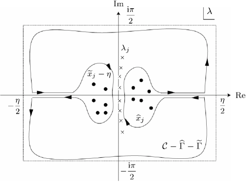
Figure 5: The integration contour $\mathcal{C}-\widehat{\Gamma}-\widetilde{\Gamma}$ corresponding to the off-critical regime $\Delta>1$.

Next step is to reduce the integrals along the contour $\mathcal{C}-\widehat{\Gamma}-\widetilde{\Gamma}$ to those along the canonical contour $\mathcal{C}$. We first consider the integrals on $\widehat{\Gamma}$. Because the integrand in (4.13) is symmetric with respect to $\{\omega\}$, we can divide the integral

$$\int_{(\mathcal{C}-\widehat{\Gamma}-\widetilde{\Gamma})^{n}}\prod_{j=1}^{n}\frac{{\rm d}\omega_{j}}{2\pi{\rm i}}\longrightarrow\sum_{k=1}^{\widehat{n}}(-1)^{k}\binom{n}{k}\int_{(\mathcal{C}-\widetilde{\Gamma})^{n-k}}\prod_{j=1}^{n-k}\frac{{\rm d}\omega_{j}}{2\pi{\rm i}}\int_{\widehat{\Gamma}^{k}}\prod_{j=1}^{k}\frac{{\rm d}\omega_{n-k+j}}{2\pi{\rm i}},$$ (4.14)

where $n=\widehat{n}+\widetilde{n}$. Note that the sum over $k$ is restricted to $k\leq\widehat{n}$, since $|{\widehat{x}}|=\widehat{n}$ and the integrand vanishes when any two of $\{\omega\}$ is the same. Noting that, inside $\widehat{\Gamma}$, $G(\omega_{j},{\widehat{x}}_{k})$ (4.7) has simple poles $\omega_{j}={\widehat{x}}_{k}$ with residues $-1$, and the poles at $\omega_{j}={\widehat{x}}_{k}$ for $\overline{M}(\omega_{j},{\widehat{x}}_{k})$ (4.6) are canceled by simple zeros of $\widehat{{\mathfrak{b}}}_{+}(\omega)$, we have

$$\int_{\widehat{\Gamma}^{k}}\prod_{j=1}^{k}\left[\frac{{\rm d}\omega_{n-k+j}}{2\pi{\rm i}(1+{\mathfrak{a}}(\omega_{j}))}\right]Y_{\widehat{n},\widetilde{n}}(\{\omega_{j}\}_{j=1}^{n}|\{x^{+}\})\widehat{Z}_{\widehat{n},\widetilde{n}}(\{\omega_{j}\}_{j=1}^{n}|\{x\})\widetilde{Z}_{\widehat{n},\widetilde{n}}(\{\omega_{j}\}_{j=1}^{n}|\{x\})$$

$$=k!\sum_{\begin{subarray}{c}\{{\widehat{x}}^{+-}\}\cup\{{\widehat{x}}^{++}\}=\{{\widehat{x}}^{+}\}\\ \{{\widehat{x}}^{++}\}\cup\{{\widetilde{x}}^{+}\}=\{x^{++}\}\\ |{\widehat{x}}^{+-}|=k\end{subarray}}\frac{Y_{\widehat{n}-k,\widetilde{n}}(\{\omega_{j}\}_{j=1}^{n-k}|\{x^{+}\})}{\prod_{j=1}^{k}(1+{\mathfrak{a}}({\widehat{x}}^{+-}_{j}))}\prod_{j=1}^{{\widetilde{m}}-\widetilde{n}}\left[1+\kappa^{-1}\overline{{\mathfrak{a}}}({\widetilde{x}}_{j}^{-})\prod_{l=1}^{n-k}\frac{f(x_{l}^{++},{\widetilde{x}}_{j}^{-})f({\widetilde{x}}_{j}^{-},\omega_{l})}{f({\widetilde{x}}_{j}^{-},x_{l}^{++})f(\omega_{l},{\widetilde{x}}_{j}^{-})}\right]$$

$$\times\prod_{j=1}^{{\widehat{m}}-\widehat{n}}\left[1+\kappa{\mathfrak{a}}({\widehat{x}}_{j}^{-})\prod_{l=1}^{n-k}\frac{f({\widehat{x}}_{j}^{-},x_{l}^{++})f(\omega_{l},{\widehat{x}}_{j}^{-})}{f(x_{l}^{++},{\widehat{x}}_{j}^{-})f({\widehat{x}}_{j}^{-},\omega_{l})}\right]\prod_{j=1}^{k}\left[1-\kappa\prod_{l=1}^{n-k}\frac{f({\widehat{x}}_{j}^{+-},x_{l}^{++})f(\omega_{l},{\widehat{x}}_{j}^{+-})}{f(x_{l}^{++},{\widehat{x}}_{j}^{+-})f({\widehat{x}}_{j}^{+-},\omega_{l})}\right].$$ (4.15)

Performing a resummation as in [11], one obtains

$$\Phi_{N}(\kappa|\{\xi\})= \sum_{\widehat{n}=0}^{{\widehat{m}}}\sum_{\widetilde{n}=0}^{{\widetilde{m}}}\sum_{\begin{subarray}{c}\{{\widehat{x}}^{+}\}\cup\{{\widehat{x}}^{-}\}=\{{\widehat{x}}\}\\ |{\widehat{x}}^{+}|=\widehat{n}\end{subarray}}\sum_{\begin{subarray}{c}\{{\widetilde{x}}^{+}\}\cup\{{\widetilde{x}}^{-}\}=\{{\widetilde{x}}\}\\ |{\widetilde{x}}^{+}|=\widetilde{n}\end{subarray}}\frac{\kappa^{{\widehat{m}}-{\widetilde{m}}-\widehat{n}}}{n!}\prod_{j=1}^{n}\frac{1}{\widehat{{\mathfrak{b}}}^{\prime}_{-}(x_{j}^{+})\widetilde{{\mathfrak{b}}}^{\prime}_{+}(x_{j}^{+})}$$

$$\times\int_{(\mathcal{C}-\widetilde{\Gamma})^{n}}\prod_{j=1}^{n}\left[\frac{{\rm d}\omega_{j}\widehat{{\mathfrak{b}}}_{-}(\omega_{j})\widetilde{{\mathfrak{b}}}_{+}(\omega_{j})}{2\pi{\rm i}(1+{\mathfrak{a}}(\omega_{j}))}\prod_{k=1}^{\widehat{n}}\frac{\operatorname{sh}(\omega_{j}-{\widehat{x}}_{k}^{+}-\eta)}{\operatorname{sh}(x_{j}^{+}-{\widehat{x}}_{k}^{+}-\eta)}\prod_{k=1}^{\widetilde{n}}\frac{\operatorname{sh}(\omega_{j}-{\widetilde{x}}_{k}^{+}+\eta)}{\operatorname{sh}(x_{j}^{+}-{\widetilde{x}}_{k}^{+}+\eta)}\right]$$

$$\times\det M(\omega_{j},x^{+}_{k})\det G(\omega_{j},x^{+}_{k})$$

$$\times\prod_{k=1}^{{\widetilde{m}}-\widetilde{n}}\frac{1}{1+{\mathfrak{a}}({\widetilde{x}}_{k}^{-})}\prod_{k=1}^{{\widetilde{m}}-\widetilde{n}}\left[1+\kappa{\mathfrak{a}}({\widetilde{x}}_{k}^{-})\prod_{j=1}^{n}\frac{f(\omega_{j},{\widetilde{x}}_{k}^{-})f({\widetilde{x}}_{k}^{-},x_{j}^{+})}{f({\widetilde{x}}_{k}^{-},\omega_{j})f(x_{j}^{+},{\widetilde{x}}_{k}^{-})}\right],$$ (4.16)

where

$$M(\omega_{j},x_{k}^{+})=t(x_{k}^{+},\omega_{j})\prod_{l=1}^{n}\frac{\operatorname{sh}(\omega_{j}-x_{l}^{+}-\eta)}{\operatorname{sh}(\omega_{j}-\omega_{l}-\eta)}+\kappa t(\omega_{j},x_{k}^{+})\prod_{l=1}^{n}\frac{\operatorname{sh}(\omega_{j}-x_{l}^{+}+\eta)}{\operatorname{sh}(\omega_{j}-\omega_{l}+\eta)}.$$ (4.17)

Now we would like to consider the integrals along the contour $\widetilde{\Gamma}$. Utilizing the relation similar to (4.14), we can separate the $\mathcal{C}$-integrals from the $\widetilde{\Gamma}$-integrals. The unwanted terms including ${\mathfrak{a}}({\widetilde{x}}_{j})$ etc, however, cannot be eliminated by actually performing the $\widetilde{\Gamma}$-integrals, since the poles inside $\widetilde{\Gamma}$ are not $\{{\widetilde{x}}\}$ but $\{{\widetilde{x}}-\eta\}$. Nevertheless, we observe that all the unwanted terms vanish in the homogeneous limit $\xi_{j}\to 0$, because the auxiliary function ${\mathfrak{a}}(\lambda)$ has poles (respectively zeros) of order $N_{0}/2+N_{1}+1$ at $\lambda=0$ (respectively $\lambda=\eta$). From the relation $\lim_{\{\xi\}\to\{0\}}G(\omega_{j},{\widetilde{x}}_{k})=-\lim_{\{\xi\}\to\{0\}}G(\omega_{j},{\widetilde{x}}_{k}-\eta)$ which is derived by adapting ${\mathfrak{a}}(0)=\infty$, ${\mathfrak{a}}(\eta)=0$ and $t(\omega,x)=t(x-\eta,\omega)$ to (4.7), we obtain

$$\Phi_{N}(\kappa|\{0\})=\lim_{\{\xi\}\to\{0\}}\sum_{\widehat{n}=0}^{{\widehat{m}}}\sum_{\widetilde{n}=0}^{{\widetilde{m}}}\sum_{\begin{subarray}{c}\{{\widehat{x}}^{+}\}\cup\{{\widehat{x}}^{-}\}=\{{\widehat{x}}\}\\ |{\widehat{x}}^{+}|=\widehat{n}\end{subarray}}\sum_{\begin{subarray}{c}\{{\widetilde{x}}^{+}\}\cup\{{\widetilde{x}}^{-}\}=\{{\widetilde{x}}\}\\ |{\widetilde{x}}^{+}|=\widetilde{n}\end{subarray}}\frac{\kappa^{m-n}}{n!}\prod_{j=1}^{n}\frac{1}{\widehat{{\mathfrak{b}}}^{\prime}_{-}(x_{j}^{+})\widetilde{{\mathfrak{b}}}^{\prime}_{+}(x_{j}^{+})}$$

$$\quad\times\int_{\mathcal{C}^{n}}\prod_{j=1}^{n}\left[\frac{{\rm d}\omega_{j}\widehat{{\mathfrak{b}}}_{-}(\omega_{j})\widetilde{{\mathfrak{b}}}_{+}(\omega_{j})}{2\pi{\rm i}(1+{\mathfrak{a}}(\omega_{j}))}\prod_{k=1}^{n}\frac{\operatorname{sh}(\omega_{j}-x_{k}^{+}-\eta)}{\operatorname{sh}(x_{j}^{+}-x_{k}^{+}-\eta)}\right]\det M(\omega_{j},x^{+}_{k})\det R(\omega_{j},x^{+}_{k}).$$ (4.18)

Here the function $R(\omega_{j},x_{k}^{+})$ is defined by

$$R(\omega_{j},x_{k}^{+})=\begin{cases}G(\omega_{j},x_{k}^{+})&\text{for $x_{k}^{+}\in\{{\widehat{x}}\}$}\\ -\kappa G(\omega_{j},x_{k}^{+}-\eta)\prod_{l=1}^{n}\frac{\operatorname{sh}(x_{k}^{+}-\omega_{l}-\eta)\operatorname{sh}(x_{k}^{+}-x_{l}^{+}+\eta)}{\operatorname{sh}(x_{k}^{+}-\omega_{l}+\eta)\operatorname{sh}(x_{k}^{+}-x_{l}^{+}-\eta)}&\text{for $x_{k}^{+}\in\{{\widetilde{x}}\}$}\end{cases},$$ (4.19)

and we have used ${\widehat{m}}-{\widetilde{m}}=m$ and $\widehat{n}+\widetilde{n}=n$. The integrand of (4.18) is a symmetric function of $\{x^{+}\}$ and vanishes at ${\widehat{x}}^{+}_{j}={\widehat{x}}^{+}_{k}$ and ${\widetilde{x}}^{+}_{j}={\widetilde{x}}^{+}_{k}$. Thanks to this together with the fact that $1/\widehat{{\mathfrak{b}}}_{-}(\lambda)$ (respectively $1/\widetilde{{\mathfrak{b}}}_{+}(\lambda)$) has simple poles at $\lambda={\widehat{x}}$ (respectively $\lambda={\widetilde{x}}$), we can directly apply (4.12) to (4.18). Thus, we finally arrive at

$$\Phi_{N}(\kappa|\{0\})= \lim_{\{\xi\}\to\{0\}}\sum_{n=0}^{{\widehat{m}}+{\widetilde{m}}}\frac{\kappa^{m-n}}{(n!)^{2}}\prod_{j=1}^{n}\left[\int_{\Gamma\{0\}\cup\Gamma\{\eta\}}\frac{{\rm d}\zeta_{j}}{2\pi{\rm i}\widehat{{\mathfrak{b}}}_{-}(\zeta_{j})\widetilde{{\mathfrak{b}}}_{+}(\zeta_{j})}\int_{\mathcal{C}}\frac{{\rm d}\omega_{j}\widehat{{\mathfrak{b}}}_{-}(\omega_{j})\widetilde{{\mathfrak{b}}}_{+}(\omega_{j})}{2\pi{\rm i}(1+{\mathfrak{a}}(\omega_{j}))}\right]$$

$$\times\prod_{j,k=1}^{n}\frac{\operatorname{sh}(\omega_{j}-\zeta_{k}-\eta)}{\operatorname{sh}(\zeta_{j}-\zeta_{k}-\eta)}\det M(\omega_{j},\zeta_{k})\det R(\omega_{j},\zeta_{k}),$$ (4.20)

where the contour $\Gamma\{0\}\cup\Gamma\{\eta\}$ surrounds the points $0$ and $\eta$ and does not contain any other singularities. In (4.20), the Trotter limit $N_{0}\to\infty$, $N_{1}\to\infty$ and the limit $\varepsilon\to 0$ can be taken analytically. In this limit, the auxiliary function ${\mathfrak{a}}(\lambda)$ is the solution to the nonlinear integral equation (3.26). Substituting (4.2) and (3.3), we easily obtain that

$$\lim_{N_{1}\to\infty}\lim_{\begin{subarray}{c}\xi\to 0\\ \varepsilon\to 0\end{subarray}}\widehat{{\mathfrak{b}}}_{-}(\lambda)\widetilde{{\mathfrak{b}}}_{+}(\lambda) =\lim_{N_{1}\to\infty}\left[\frac{\operatorname{sh}(\lambda+\beta_{1}/N_{1})}{\operatorname{sh}(\lambda+\beta_{1}/N_{1}-\eta)}\right]^{\frac{N_{1}}{2}}\left[\frac{\operatorname{sh}(\lambda-\eta)}{\operatorname{sh}(\lambda)}\right]^{\frac{N_{1}}{2}}\left[\frac{\operatorname{sh}\lambda}{\operatorname{sh}(\lambda-\eta)}\right]^{m}$$

$$=\exp\left[-{\rm i}te\left(\lambda-\frac{\eta}{2}\right)-{\rm i}mp\left(\lambda-\frac{\eta}{2}\right)\right],$$ (4.21)

where $e(\lambda)$ and $p(\lambda)$ are related to the bare one-particle energy and momentum, respectively. They are explicitly given by

$$e(\lambda)=\frac{2J\operatorname{sh}^{2}\eta}{\operatorname{sh}(\lambda+\frac{\eta}{2})\operatorname{sh}(\lambda-\frac{\eta}{2})},\quad p(\lambda)={\rm i}\ln\left(\frac{\operatorname{sh}(\lambda+\frac{\eta}{2})}{\operatorname{sh}(\lambda-\frac{\eta}{2})}\right).$$ (4.22)

From (4.20), (4.3) and (3.16), we end up with the following theorem.

Theorem 1

The generating function of the longitudinal dynamical correlation function has the following multiple integral representation:

$$\mathcal{Q}_{\kappa}(m,t)=\sum_{n=0}^{\infty}\frac{\kappa^{m-n}}{(n!)^{2}}\prod_{j=1}^{n}\left[\int_{\Gamma\{0\}\cup\Gamma\{\eta\}}\frac{{\rm d}\zeta_{j}}{2\pi{\rm i}}\int_{\mathcal{C}}\frac{{\rm d}\omega_{j}}{2\pi{\rm i}(1+{\mathfrak{a}}(\omega_{j}))}\right]\prod_{j,k=1}^{n}\frac{\operatorname{sh}(\omega_{j}-\zeta_{k}-\eta)}{\operatorname{sh}(\zeta_{j}-\zeta_{k}-\eta)}$$

$$\quad\times\prod_{j=1}^{n}{\rm e}^{{\rm i}t(e(\zeta_{j}-\frac{\eta}{2})-e(\omega_{j}-\frac{\eta}{2}))+{\rm i}m(p(\zeta_{j}-\frac{\eta}{2})-p(\omega_{j}-\frac{\eta}{2}))}\det M(\omega_{j},\zeta_{k})\det R(\omega_{j},\zeta_{k}).$$ (4.23)

In this expression the function ${\mathfrak{a}}(\lambda)$ is the solution to the nonlinear integral equation (3.26); $e(\lambda)$ and $p(\lambda)$, respectively, denote the bare one-particle energy and momentum (4.22); the function $M(\omega,\zeta)$ and $R(\omega,\zeta)$ are, respectively, defined by

$$M(\omega,\zeta) =t(\zeta,\omega)\prod_{l=1}^{n}\frac{\operatorname{sh}(\omega-\zeta_{l}-\eta)}{\operatorname{sh}(\omega-\omega_{l}-\eta)}+\kappa t(\omega,\zeta)\prod_{l=1}^{n}\frac{\operatorname{sh}(\omega-\zeta_{l}+\eta)}{\operatorname{sh}(\omega-\omega_{l}+\eta)},$$

$$R(\omega,\zeta) =\begin{cases}G(\omega,\zeta)&\text{for $\zeta\sim 0$}\\ -\kappa G(\omega,\zeta-\eta)\prod_{l=1}^{n}\frac{\operatorname{sh}(\zeta-\omega_{l}-\eta)\operatorname{sh}(\zeta-\zeta_{l}+\eta)}{\operatorname{sh}(\zeta-\omega_{l}+\eta)\operatorname{sh}(\zeta-\zeta_{l}-\eta)}&\text{for $\zeta\sim\eta$}\end{cases},$$ (4.24)

where $t(\lambda,\mu)=\operatorname{sh}(\eta)/(\operatorname{sh}(\lambda-\mu)\operatorname{sh}(\lambda-\mu+\eta))$ and $G(\lambda,\zeta)$ is the solution of the linear integral equation

$$G(\lambda,\zeta)=t(\zeta,\lambda)+\int_{\mathcal{C}}\frac{{\rm d}\omega}{2\pi{\rm i}}\frac{\operatorname{sh}(2\eta)}{\operatorname{sh}(\lambda-\omega+\eta)\operatorname{sh}(\lambda-\omega-\eta)}\frac{G(\omega,\zeta)}{1+{\mathfrak{a}}(\omega)}.$$ (4.25)

The contour $\mathcal{C}$ is the canonical contour (see figure 4) and $\Gamma\{0\}\cup\Gamma\{\eta\}$ encircles the points $0$ and $\eta$.

Thus the time-dependent longitudinal correlation function $\langle\sigma_{1}^{z}(0)\sigma_{m+1}^{z}(t)\rangle$ can be evaluated by inserting the generating function (4.23) into (3.17), and using the magnetization

$$\langle\sigma^{z}\rangle=-1-\int_{\mathcal{C}}\frac{{\rm d}\omega}{\pi{\rm i}}\frac{G(\omega,0)}{1+{\mathfrak{a}}(\omega)}=1+\int_{\mathcal{C}}\frac{{\rm d}\omega}{\pi{\rm i}}\frac{G(\omega,0)}{1+\overline{{\mathfrak{a}}}(\omega)},$$ (4.26)

which is derived from (3.26), (3.27), (3.29) and (4.25) [11].

5 Special cases

Here we comment on some special cases derived from the multiple integral representation (4.23) for the dynamical correlation function $\langle\sigma_{1}^{z}(0)\sigma_{m+1}^{z}(t)\rangle$.

5.1 Static limit $t=0$

First let us consider the static limit $t=0$. Due to the factors $e(\zeta_{j}-\eta/2)$, the integrand in (4.23) has essential singularities located on $\zeta_{j}=0$ and $\eta$. In the static limit these essential singularities vanish, and hence the integrals along the contour $\Gamma\{\eta\}$ disappear. Because the remaining part of the integrand has poles of order $m$ at the points $\zeta_{j}=0$, the integrals on the contour $\Gamma\{0\}$ vanish for $n>m$. Namely the sum over $n$ is restricted to $n\leq m$. The resultant expression reads

$$\mathcal{Q}_{\kappa}(m,0)= \sum_{n=0}^{m}\frac{\kappa^{m-n}}{(n!)^{2}}\prod_{j=1}^{n}\left[\int_{\Gamma\{0\}}\frac{{\rm d}\zeta_{j}}{2\pi{\rm i}}\left\{\frac{\operatorname{sh}(\zeta_{j}-\eta)}{\operatorname{sh}(\zeta_{j})}\right\}^{m}\int_{\mathcal{C}}\frac{{\rm d}\omega_{j}}{2\pi{\rm i}(1+{\mathfrak{a}}(\omega_{j}))}\left\{\frac{\operatorname{sh}(\omega_{j})}{\operatorname{sh}(\omega_{j}-\eta)}\right\}^{m}\right]$$

$$\times\prod_{j,k=1}^{n}\frac{\operatorname{sh}(\omega_{j}-\zeta_{k}-\eta)}{\operatorname{sh}(\zeta_{j}-\zeta_{k}-\eta)}\det M(\omega_{j},\zeta_{k})\det G(\omega_{j},\zeta_{k}),$$ (5.1)

agreeing with that in [11].

5.2 Zero-temperature limit $T=0$

For direct comparison with the previous result for $T=0$ [9], it is convenient to introduce another expression of the generating function. Considering the correlation function $\langle\sigma_{m+1}^{z}(-t)\sigma_{1}(0)\rangle$ which is equivalent to $\langle\sigma^{z}_{1}(0)\sigma^{z}_{m+1}(t)\rangle$, and utilizing the technique described in the previous section, one may obtain

$$\mathcal{Q}_{\kappa}(m,t)=\sum_{n=0}^{\infty}\frac{(-1)^{n}}{(n!)^{2}}\prod_{j=1}^{n}\left[\int_{\Gamma\{-\eta\}\cup\Gamma\{0\}}\frac{{\rm d}\zeta_{j}}{2\pi{\rm i}}\int_{\mathcal{C}}\frac{{\rm d}\omega_{j}}{2\pi{\rm i}(1+\overline{{\mathfrak{a}}}(\omega_{j}))}\right]\prod_{j,k=1}^{n}\frac{\operatorname{sh}(\omega_{j}-\zeta_{k}+\eta)}{\operatorname{sh}(\zeta_{j}-\zeta_{k}+\eta)}$$

$$\quad\times\prod_{j=1}^{n}{\rm e}^{{\rm i}t(e(\zeta_{j}+\frac{\eta}{2})-e(\omega_{j}+\frac{\eta}{2}))+{\rm i}m(\overline{p}(\zeta_{j}+\frac{\eta}{2})-\overline{p}(\omega_{j}+\frac{\eta}{2}))}\det M(\omega_{j},\zeta_{k})\det\overline{R}(\omega_{j},\zeta_{k}),$$ (5.2)

where $\overline{p}(\lambda)$ and $\overline{R}(\omega,\zeta)$ are defined by

$$\overline{p}(\lambda)={\rm i}\ln\left(\frac{\operatorname{sh}(\lambda-\frac{\eta}{2})}{\operatorname{sh}(\lambda+\frac{\eta}{2})}\right),$$

$$\overline{R}(\omega,\zeta)=\begin{cases}G(\omega,\zeta)&\text{for $\zeta\sim 0$}\\ -\kappa^{-1}G(\omega,\zeta+\eta)\prod_{l=1}^{n}\frac{\operatorname{sh}(\zeta-\omega_{l}+\eta)\operatorname{sh}(\zeta-\zeta_{l}-\eta)}{\operatorname{sh}(\zeta-\omega_{l}-\eta)\operatorname{sh}(\zeta-\zeta_{l}+\eta)}&\text{for $\zeta\sim-\eta$}\end{cases}.$$ (5.3)

Note that $G(\lambda,\zeta)$ is the solution of the integral equation (4.7) which is also written in terms of $\overline{{\mathfrak{a}}}(\lambda)$ if $\lambda$ and $\zeta$ are located inside $\mathcal{C}$:

$$G(\lambda,\zeta)=-t(\lambda,\zeta)-\int_{\mathcal{C}}\frac{{\rm d}\omega}{2\pi{\rm i}}\frac{\operatorname{sh}(2\eta)}{\operatorname{sh}(\lambda-\omega+\eta)\operatorname{sh}(\lambda-\omega-\eta)}\frac{G(\omega,\zeta)}{1+\overline{{\mathfrak{a}}}(\omega)}.$$ (5.4)

Here we restrict ourselves on the off-critical case $\Delta>0$ and set $\eta<0$ as in [9]. Note that we can also treat the critical case $|\Delta|\leq 1$ by just changing the definition of the integration contour as in figure 4.

Shifting the variables in (5.2) by $\omega_{j}\to\omega_{j}-\eta/2$ and $\zeta_{j}\to\zeta_{j}-\eta/2$, we consider the integrals on the contour $\Gamma\{-\eta/2\}\cup\Gamma\{\eta/2\}$ and $-\mathcal{C}_{0}\cup\mathcal{C}_{\frac{\eta}{2}}$. Here $\mathcal{C}_{0}$ and $\mathcal{C}_{\frac{\eta}{2}}$ denote $\mathcal{C}_{0}=[-\pi{\rm i}/2,\pi{\rm i}/2]$ and $\mathcal{C}_{\frac{\eta}{2}}=[\eta/2-\pi{\rm i}/2,\eta/2+\pi{\rm i}/2]$, respectively. By close analysis of the auxiliary function $\overline{{\mathfrak{a}}}(\lambda)$ for $h>0$ and $\eta<0$ at the zero-temperature limit $T\to 0$, one finds

$$\frac{1}{1+\overline{{\mathfrak{a}}}(\lambda)}\xrightarrow{T\to 0}\begin{cases}0&\text{for $\lambda\in\mathcal{C}_{0}\cup\mathcal{C}_{\frac{\eta}{2}}\setminus\mathcal{L}$}\\ 1&\text{for $\lambda\in\mathcal{L}$}\end{cases},\quad\mathcal{L}\in\left[-q_{h}+\frac{\eta}{2},q_{h}+\frac{\eta}{2}\right],$$ (5.5)

where the ‘Fermi point’ $q_{h}$ is an imaginary number depending on $h$. Substituting this into (5.4) and appropriately shifting the variables, we have

$$G\left(\lambda-\frac{\eta}{2},\zeta-\frac{\eta}{2}\right)=-t(\lambda,\zeta)+\int_{-\mathcal{L}}\frac{{\rm d}\omega}{2\pi{\rm i}}\frac{\operatorname{sh}(2\eta)G\left(\omega-\frac{\eta}{2},\zeta-\frac{\eta}{2}\right)}{\operatorname{sh}(\lambda-\omega+\eta)\operatorname{sh}(\lambda-\omega-\eta)}.$$ (5.6)

Comparing above with equation (2.16) in [7], one identifies $G(\lambda,\zeta)$ as the density function $\rho(\lambda,\zeta)$:

$$G\left(\lambda-\frac{\eta}{2},\zeta-\frac{\eta}{2}\right)=2\pi{\rm i}\rho(\lambda,\zeta).$$ (5.7)

Inserting (5.7) and (5.5) into (5.2), we arrive at the expression for the generating function at $T=0$:

$$\lim_{T\to 0}\mathcal{Q}_{\kappa}(m,t)= \sum_{n=0}^{\infty}\frac{1}{(n!)^{2}}\prod_{j=1}^{n}\left[\int_{\Gamma\{\pm\eta/2\}}\frac{{\rm d}\zeta_{j}}{2\pi{\rm i}}\int_{-\mathcal{L}}{\rm d}\omega_{j}\right]\prod_{j,k=1}^{n}\frac{\operatorname{sh}(\omega_{j}-\zeta_{k}+\eta)}{\operatorname{sh}(\zeta_{j}-\zeta_{k}+\eta)}$$

$$\quad\times\prod_{j=1}^{n}{\rm e}^{{\rm i}t(e(\zeta_{j})-e(\omega_{j}))+{\rm i}m(\overline{p}(\zeta_{j})-\overline{p}(\omega_{j}))}\det M(\omega_{j},\zeta_{k})\det\mathcal{R}(\omega_{j},\zeta_{k})$$ (5.8)

with

$$\mathcal{R}(\omega,\zeta)=\begin{cases}\rho(\omega,\zeta)&\text{for $\zeta\sim 0$}\\ -\kappa^{-1}\rho(\omega,\zeta+\eta)\prod_{j=1}^{n}\frac{\operatorname{sh}(\zeta-\omega_{l}+\eta)\operatorname{sh}(\zeta-\zeta_{l}-\eta)}{\operatorname{sh}(\zeta-\omega_{l}-\eta)\operatorname{sh}(\zeta-\zeta_{l}+\eta)}&\text{for $\zeta\sim-\eta$}\end{cases}.$$ (5.9)

The above expression reproduces equation (6.17) in [9].

5.3 XY (free fermion) limit $\Delta=0$

Along the method described in [9] (see also [24, 25] for the static case), we would like to study the XY limit, where $\langle\sigma_{1}^{z}(0)\sigma_{m+1}^{z}(t)\rangle$ can be written as a product of single integrals. Set $\eta=\pi{\rm i}/2$. Then the kernels of the integral equation in $\eqref{nlie1}$ and in $\eqref{G-function2}$ are equal to zero. Hence

$${\mathfrak{a}}(\lambda)=\exp\left[-\frac{h}{T}-\frac{1}{T}\frac{4{\rm i}J}{\operatorname{sh}(2\lambda)}\right],\quad G(\lambda,\zeta)=\frac{-2}{\operatorname{sh}(2(\lambda-\zeta))}.$$ (5.10)

Shifting the variables $\zeta_{j}\to\zeta_{j}+\pi{\rm i}/4$ and $\omega_{j}\to\omega_{j}+\pi{\rm i}/4$ in (4.23), one easily sees

$$\mathcal{Q}_{\kappa}(m,t)=\sum_{n=0}^{\infty} \frac{\kappa^{m-n}}{(n!)^{2}}\prod_{j=1}^{n}\left[\int_{\Gamma\{\pm\pi{\rm i}/4\}}\frac{{\rm d}\zeta_{j}}{2\pi{\rm i}}\int_{\mathcal{C^{\prime}}}\frac{{\rm d}\omega_{j}}{2\pi{\rm i}(1+{\mathfrak{a}}(\omega_{j}+\frac{\pi}{4}{\rm i}))}\right]\prod_{j,k=1}^{n}\frac{\operatorname{ch}(\omega_{j}-\zeta_{k})}{\operatorname{ch}(\zeta_{j}-\zeta_{k})}$$

$$\times\prod_{j=1}^{n}{\rm e}^{{\rm i}t(e(\zeta_{j})-e(\omega_{j}))+{\rm i}m(p(\zeta_{j})-p(\omega_{j}))}\det M(\omega_{j},\zeta_{k})\det R(\omega_{j},\zeta_{k}),$$ (5.11)

where $\mathcal{C^{\prime}}=-\mathcal{C}_{0}\cup\mathcal{C}_{-\pi{\rm i}/2}$; $\mathcal{C}_{0}=[-\infty,\infty]$; $\mathcal{C}_{-\pi{\rm i}/2}=[-\pi{\rm i}/2-\infty,-\pi{\rm i}/2+\infty]$. In this case the function $R(\omega,\zeta)$ and $M(\omega,\zeta)$ are reduced to

$$R(\omega,\zeta)=\begin{cases}-\frac{2}{\operatorname{sh}(2(\omega-\zeta))}&\text{ for $\zeta\sim\pi{\rm i}/4$}\\ -\kappa\frac{2}{\operatorname{sh}(2(\omega-\zeta))}&\text{ for $\zeta\sim-\pi{\rm i}/4$}\end{cases},\,\,M(\omega,\zeta)=\frac{2(\kappa-1)}{\operatorname{sh}(2(\omega-\zeta))}\prod_{l=1}^{n}\frac{\operatorname{ch}(\omega-\zeta_{l})}{\operatorname{ch}(\omega-\omega_{l})}.$$ (5.12)

In the above expression, we notice that $M(\omega,\zeta)$ is factorized and has the factor $\kappa-1$, which significantly simplifies the integral representation. After taking the second derivative with respect to $\kappa$ and setting $\kappa=1$, one observes all the terms $n>2$ vanish. Firstly we consider the case $n=2$. Substituting (5.12) into (5.11), we extract the term corresponding to $n=2$ (written as $\mathcal{Q}^{(2)}_{\kappa}(m,t)$). After differentiating with respect to $\kappa$ and setting $\kappa=1$, one has

$$\partial^{2}_{\kappa}\mathcal{Q}^{(2)}_{\kappa}(m,t)\Bigr{|}_{\kappa=1}$$

$$\,\,=\frac{1}{32\pi^{4}}\prod_{j=1}^{2}\left[\int_{\mathcal{C}^{\prime}}\frac{{\rm d}\omega_{j}}{1+{\mathfrak{a}}(\omega_{j}+\frac{\pi{\rm i}}{4})}\int_{\Gamma\{\pm\pi{\rm i}/4\}}{\rm d}\zeta_{j}\right]\det\left[\frac{{\rm e}^{{\rm i}te(\zeta_{k})+{\rm i}mp(\zeta_{k})}}{\operatorname{sh}(\omega_{j}-\zeta_{k})}\right]\det\left[\frac{{\rm e}^{-{\rm i}te(\omega_{j})-{\rm i}mp(\omega_{j})}}{\operatorname{sh}(\omega_{j}-\zeta_{k})}\right].$$ (5.13)

The integral on $\Gamma\{\pm\pi{\rm i}/4\}$ can be evaluated by considering the residues outside the contour $\Gamma\{\pm\pi{\rm i}/4\}$ i.e. at the points $\zeta_{j}=\omega_{k}$. This leads to

$$\partial^{2}_{\kappa}\mathcal{Q}^{(2)}_{\kappa}(m,t)\Bigr{|}_{\kappa=1}=\frac{-1}{4\pi^{2}}\prod_{j=1}^{2}\left[\int_{\mathcal{C}^{\prime}}\frac{{\rm d}\omega_{j}}{1+{\mathfrak{a}}(\omega_{j}+\frac{\pi{\rm i}}{4})}\right]\det\left[\frac{1-{\rm e}^{{\rm i}t(e(\omega_{j})-e(\omega_{k}))+{\rm i}m(p(\omega_{j})-p(\omega_{k}))}}{\operatorname{sh}(\omega_{j}-\omega_{k})}\right].$$ (5.14)

Changing the variables $\cosh(2\omega)=-1/\cos p$ and identifying

$${\rm d}\omega=\frac{\operatorname{ch}(2\omega)}{2}{\rm d}p,\quad e(\omega)=4J\cos p,\quad\frac{\sqrt{\operatorname{ch}(2\omega_{j})\operatorname{ch}(2\omega_{k})}}{\operatorname{sh}(\omega_{j}-\omega_{k})}=\frac{1}{\sin\frac{1}{2}(p_{j}-p_{k})},$$ (5.15)

one obtains

$$\partial^{2}_{\kappa}\mathcal{Q}^{(2)}_{\kappa}(m,t)\Bigr{|}_{\kappa=1}=\frac{-1}{16\pi^{2}}\prod_{j=1}^{2}\left[\int_{-\pi}^{\pi}{\rm d}p_{j}\vartheta(p_{j})\right]\det\left[\frac{1-{\rm e}^{4{\rm i}tJ(\cos p_{j}-\cos p_{k})+{\rm i}m(p_{j}-p_{k})}}{\sin\frac{1}{2}(p_{j}-p_{k})}\right],$$ (5.16)

where $\vartheta(p)$ is the Fermi distribution function

$$\vartheta(p)=\frac{1}{1+\exp[-\frac{h}{T}+\frac{4J\cos p}{T}]}.$$ (5.17)

Taking the lattice derivative over $m$, we obtain the following relation, without explicit evaluation of the multiple integral:

$$2D_{m}^{2}\partial^{2}_{\kappa}\mathcal{Q}^{(2)}_{\kappa}(m,t)\Bigr{|}_{\kappa=1}=\frac{1}{\pi^{2}}\left[\int_{-\pi}^{\pi}{\rm d}p\vartheta(p)\right]^{2}-\frac{1}{\pi^{2}}\left|\int_{-\pi}^{\pi}{\rm d}p\vartheta(p){\rm e}^{4{\rm i}tJ\cos p+{\rm i}mp}\right|^{2}.$$ (5.18)

Next let us compute the term $\mathcal{Q}^{(1)}_{\kappa}(m,t)$ corresponding to $n=1$. Its explicit form is

$$\mathcal{Q}^{(1)}_{\kappa}(m,t)=\frac{\kappa^{m-1}(\kappa-1)}{4\pi^{2}} \left[\int_{\Gamma\{-\pi{\rm i}/4\}}{\rm d}\zeta+\kappa\int_{\Gamma\{\pi{\rm i}/4\}}{\rm d}\zeta\right]$$

$$\times\int_{\mathcal{C}^{\prime}}\frac{{\rm d}\omega}{1+{\mathfrak{a}}(\omega+\frac{\pi{\rm i}}{4})}\frac{{\rm e}^{{\rm i}t(e(\zeta)-e(\omega))+{\rm i}m(p(\zeta)-p(\omega))}}{\operatorname{sh}^{2}(\omega-\zeta)}.$$ (5.19)

Evaluating the integral on $\Gamma\{\pm\pi{\rm i}/4\}$, one has

$$\left[\int_{\Gamma\{-\pi{\rm i}/4\}}{\rm d}\zeta+\int_{\Gamma\{\pi{\rm i}/4\}}{\rm d}\zeta\right]\frac{{\rm e}^{{\rm i}t(e(\zeta)-e(\omega))+{\rm i}m(p(\zeta)-p(\omega))}}{\operatorname{sh}^{2}(\omega-\zeta)}=2\pi[te^{\prime}(\omega)+mp^{\prime}(\omega)].$$ (5.20)

It immediately follows that

$$2D_{m}^{2}\partial_{\kappa}^{2}\mathcal{Q}^{(1)}_{\kappa}(m,t)\Bigr{|}_{\kappa=1}= \frac{4}{\pi^{2}}\int_{\Gamma\{-\pi{\rm i}/4\}}{\rm d}\zeta\int_{\mathcal{C}^{\prime}}\frac{{\rm d}\omega}{1+{\mathfrak{a}}(\omega+\frac{\pi{\rm i}}{4})}\frac{{\rm e}^{{\rm i}t(e(\zeta)-e(\omega))+{\rm i}m(p(\zeta)-p(\omega))}}{\operatorname{ch}(2\omega)\operatorname{ch}(2\zeta)}$$

$$\quad+\frac{4}{\pi}\int_{\mathcal{C}^{\prime}}\frac{{\rm d}\omega}{1+{\mathfrak{a}}(\omega+\frac{\pi{\rm i}}{4})}p^{\prime}(\omega).$$ (5.21)

The contour $\Gamma\{-\pi{\rm i}/4\}$ in the first term can be replaced by $\mathcal{C}^{\prime}$. After changing variables as in (5.15), one arrives at

$$2D_{m}^{2}\partial_{\kappa}^{2}\mathcal{Q}^{(1)}_{\kappa}(m,t)\Bigr{|}_{\kappa=1}=\frac{1}{\pi^{2}}\int_{-\pi}^{\pi}{\rm d}p\vartheta(p){\rm e}^{-4{\rm i}tJ\cos p-{\rm i}mp}\int_{-\pi}^{\pi}{\rm d}q{\rm e}^{4{\rm i}tJ\cos q+{\rm i}mq}-\frac{4}{\pi}\int_{-\pi}^{\pi}{\rm d}p\vartheta(p).$$ (5.22)

Sum up (5.18), (5.22) and $2D_{m}^{2}\partial_{\kappa}\mathcal{Q}^{(0)}(m,t)|_{\kappa=1}=4$ which is trivially obtained from $\mathcal{Q}^{(0)}(m,t)=\kappa^{m}$. Then inserting the result into (3.17) and using the magnetization (see (4.26)):

$$\langle\sigma^{z}\rangle=-1+\frac{1}{\pi}\int_{-\pi}^{\pi}{\rm d}p\vartheta(p),$$ (5.23)

we finally obtain

$$\langle\sigma_{1}^{z}(0)\sigma_{m+1}^{z}(t)\rangle= \langle\sigma^{z}\rangle^{2}-\frac{1}{\pi^{2}}\left|\int_{-\pi}^{\pi}{\rm d}p\vartheta(p){\rm e}^{4{\rm i}tJ\cos p+{\rm i}mp}\right|^{2}$$

$$\quad+\frac{1}{\pi^{2}}\int_{-\pi}^{\pi}{\rm d}p\vartheta(p){\rm e}^{-4{\rm i}tJ\cos p-{\rm i}mp}\int_{-\pi}^{\pi}{\rm d}q{\rm e}^{4{\rm i}tJ\cos q+{\rm i}mq}.$$ (5.24)

The above expression coincides with the known result as in [15]. Of course, (5.24) can also be derived by starting from the generating function defined in (5.2).

6 Conclusion

In this paper, we have derived a multiple integral representation for the time-dependent longitudinal correlation function $\langle\sigma_{1}^{z}(0)\sigma_{m+1}^{z}(t)\rangle$ at any finite temperature and finite magnetic field. The formula reproduces the known results in the following three limits: (i) static limit, (ii) low-temperature limit and (iii) XY limit.

It will be very interesting to consider the following problems which still remain open. First, it is well-known that the long-distance asymptotics of correlation functions at the low-energy region (namely $T=0$ or $T\ll J$) in the critical regime can be derived by a field theoretical argument (see [26] for example). In contrast, our multiple integral representation (4.23) is valid for any finite temperature and interaction strength. The exact computations of the asymptotic behavior from (4.23) beyond the field theoretical predictions are of importance.

Second, how do we evaluate and extract the long-time asymptotics of the correlation function $\langle\sigma_{1}^{z}(0)\sigma_{m+1}^{z}(t)\rangle$ at infinite temperature? In this case the auxiliary function ${\mathfrak{a}}(\lambda)$ in (4.23) becomes quite simple: ${\mathfrak{a}}(\lambda)=1$. This problem is of interest in relation to the issue of spin-diffusion in the spin-1/2 Heisenberg XXZ chain (see, for example, [27, 28, 29, 30]).

The third is how to apply our formula to the calculation of crucial physical quantities such as the dynamical spin structure factor [31, 32, 33, 34, 35, 36], which can be actually measured by a neutron scattering experiment. In relation to this problem, finally we would like to comment on the form factor expansion. In fact, the multiple integral representation for $T=0$ (see (5.8)) is directly connected to the form factor expansion [9, 8]. On the other hand, for the finite temperature case, it is not clear whether (4.23) has a connection with the form factor expansion, since (4.23) is derived by the quantum transfer matrix acting not on the quantum space but on the auxiliary space. The form factor expansion is an important tool to investigate the dynamical properties of the system, and therefore explicit expressions at finite temperature are also desired.

References

[1] M. Jimbo, K. Miki, T. Miwa, and A. Nakayashiki,
Phys. Lett. A 168 (1992) 256.
[2] M. Jimbo and T. Miwa, Algebraic Analysis of
Solvable Lattice Models, (American Mathematical Society,
Providence, RI, 1995).
[3] A. Nakayashiki, Int. J. Mod. Phys. A 9 (1994)
5673.
[4] V.E. Korepin, A.G. Izergin, F.H.L. Essler, and D.B. Uglov,
Phys. Lett. A 190 (1994) 182.
[5] M. Jimbo and T. Miwa, J. Phys. A 29 (1996) 2923.
[6] N. Kitanine, J. M. Maillet and
V. Terras, Nucl. Phys. B 567 (2000) 554.
[7] N. Kitanine, J. M. Maillet,
N. A. Slavnov and V. Terras, Nucl. Phys. B
641 (2002) 487.
[8] N. Kitanine, J. M. Maillet,
N. A. Slavnov and V. Terras, Nucl. Phys. B
712 (2005) 600.
[9] N. Kitanine, J. M. Maillet,
N. A. Slavnov and V. Terras, Nucl. Phys. B
729 (2005) 558.
[10] N. Kitanine, J. M. Maillet,
N. A. Slavnov and V. Terras, hep-th/0505006.
[11] F. Göhmann, A. Klümper and
A. Seel, J. Phys. A 37 (2004) 7625.
[12] F. Göhmann, A. Klümper and
A. Seel, J. Phys. A 38 (2005) 1833.
[13] F. Göhmann and N. P. Hasenclever
and A. Seel,
J. Stat. Mech. 0510 (2005) P10015.
[14] H. E. Boos, F. Göhmann, A. Klümper
and J. Suzuki, J. Stat. Mech. 0604 (2006) P04001.
[15] F. Colomo, A.G. Izergin, V. E. Korepin,
V. Tognetti, Theor. Math. Phys. 94 (1993) 11.
[16] N. Kitanine, J. M. Maillet and
V. Terras, Nucl. Phys. B 554 (1999) 647.
[17] J. M. Maillet and V. Terras,
Nucl. Phys. B 575 (2000) 627.
[18] F. Göhmann and V.E. Korepin,
J. Phys. A 33 (2000) 1199.
[19]
M. Suzuki, Phys. Rev. B 31 (1985) 2957.
[20]
M. Suzuki and M. Inoue, Prog. Theor. Phys.
78 (1987) 787.
[21]
A. Klümper, Ann. Phys., Lpz. 1 (1992) 540.
[22]
A. Klümper, Z. Phys. B 91 (1993) 507.
[23]
C. Destri and de H. J. de Vega, Phys. Rev. Lett.
69 (1992) 2313.
[24] N. Kitanine, J. M. Maillet,
N. A. Slavnov and V. Terras, Nucl. Phys. B
642 (2002) 433.
[25] F. Göhmann and A. Seel,
Theor. and Math. Phys. 146 (2006) 119.
[26]
V.E. Korepin, N.M. Bogoliubov and A.G. Izergin, Quantum Inverse Scattering Method and Correlation
Functions (Cambridge University Press, Cambridge, 1993).
[27] K. Fabricius, U Löw and J. Stolze,
Phys. Rev. B 55 (1997) 5833.
[28] K. Fabricius and B.M. McCoy, Phys. Rev. B 57 (1998)
8340.
[29] S. Glocke, A. Klümper and J. Sirker, cond-mat/0610689.
[30] J. Sirker, Phys. Rev. B 73 (2006) 224424.
[31]
D. Biegel, M. Karbach and G. Müller, Europhys. Lett. 59
(2002) 882.
[32] J. Sato and M. Shiroishi,
J. Phys. Soc. Jpn. 73 (2004) 3008.
[33] J.-S. Caux, R. Hagemans, J.-M. Maillet,
J. Stat. Mech. (2005) P09003.
[34] J.-S. Caux and J. M. Maillet,
Phys. Rev. Lett. 95 (2005) 077201.
[35] R. G. Pereira,
J. Sirker, J.-S. Caux, R. Hagemans, J. M. Maillet, S. R. White,
I. Affleck, Phys. Rev. Lett. 96 (2006) 257202.
[36] J.-S. Caux and R. Hagemans,
J. Stat. Mech. 0612 (2006) P12013.