Local density of states at zigzag edge of carbon nanotubes and graphene

Abstract

The electron-phonon matrix element for edge states of carbon nanotubes and graphene at zigzag edges is calculated for obtaining renormalized energy dispersion of the edge states. Self-energy correction by electron-phonon interaction contributes to the energy dispersion of edge states whose energy bandwidth is similar to phonon energy. Since the energy-uncertainty of the edge state is larger than temperature, we conclude that the single-particle picture of the edge state in not appropriate when the electron-phonon interaction is taken into account. The longitudinal acoustic phonon mode contributes to the matrix element through the on-site deformation potential because the wavefunction of the edge state has an amplitude only on one of the two sublattices. The on-site deformation potentials for the longitudinal and in-plane tangential optical phonon modes are enhanced at the boundary. The results of local density of states are compared with the recent experimental data of scanning tunneling spectroscopy.

I introduction

The local electronic property near the edge of graphene depends on the lattice structure of the edge. For example, the zigzag edge induces edge states which are $\pi$-electron states localized near the edge while the armchair edge does not. Fujita et al. (1996) The edge states which have a flat energy dispersion, show a peak in local density of states (LDOS) near the Fermi energy. The peak structure in LDOS has been observed at the edge of graphene by scanning tunneling microscopy (STM) and spectroscopy (STS). Niimi et al. (2005, 2006); Kobayashi et al. (2005, 2006) The LDOS peak is a direct evidence of the edge states because the peak is not observed at an armchair edge and the height of the peak decreases with increasing a distance of the STS tip on graphene plane from the zigzag edge. The data on LDOS are useful to understand the energy and life-time of an electron in the edge states. The life-time of the electron is determined by electron-phonon (el-ph) interaction and the el-ph interaction is important for almost flat energy dispersion when the Debye energy ($\hbar\omega_{\rm D}\approx 0.2$ eV) is comparable to the energy bandwidth. Thus the el-ph interaction for edge states affects STS spectra and is essential for an analysis of STS. In this paper, we consider self-energy correction for edge states induced by the el-ph interaction, and compare the theoretical results of LDOS with experimental data. Niimi et al. (2005, 2006); Kobayashi et al. (2005)

A complete flat energy dispersion relation of the edge states is widely recognized by the theory. Fujita et al. (1996) However, STM/STS Niimi et al. (2005, 2006); Kobayashi et al. (2005, 2006) and angle-resolved photo-emission spectroscopy (ARPES) Sugawara et al. (2006) show that the edge states have a small but finite energy dispersion. Using STM/STS at graphene edge, Niimi et al. Niimi et al. (2005, 2006) and Kobayashi et al. Kobayashi et al. (2005, 2006) independently observed a peak in the LDOS below the Fermi energy by 20 $\sim$ 30 meV. The peak position relative to the Fermi point ($E_{\rm F}=0$) shows that the edge states have a finite bandwidth. Using ARPES, Sugawara et al., Sugawara et al. (2006) observed the Fermi surface of Kish graphite and found a weakly dispersive energy band near the Fermi energy. In the previous paper, we pointed out that next nearest-neighbor (nnn) tight-binding Hamiltonian, ${\cal H}_{\rm nnn}$, is essential for the bandwidth. Sasaki et al. (2006) As shown in Sec. II, ${\cal H}_{\rm nnn}$ lowers the energy dispersion of the edge states as $E(k)=\gamma_{n}(2\cos ka+1)$ ($2\pi/3<ka<4\pi/3$) where $\gamma_{n}$ and $a$ is the hopping integral between nnn sites ($\gamma_{n}\sim 0.3$ eV) and a lattice constant of graphite ($a=2.46$ Å), and the value of $\gamma_{n}$ is calculated on the basis of density-functional theory by Porezag et al. Porezag et al. (1995) Since $ka=\pi$ state is located at the bottom of the band and $ka\to 2\pi/3$ (or $4\pi/3$) is located at the top of the band, the bandwidth of the edge states, $W$, is given by $W=\gamma_{n}$. However, the observed energy bandwidth (20 $\sim$ 30 meV) is much smaller than $\gamma_{n}$. The reason why observed bandwidth is smaller than $\gamma_{n}$ is that the self-energy correction $\Sigma(k)$ renormalizes $E(k)$ as $E(k)+{\rm Re}(\Sigma(k))$. Because the el-ph interaction makes the effective mass of the edge states large, $W$ generally decreases by taking account of el-ph interaction. It is also noted that $\Gamma(k)\equiv-2{\rm Im}(\Sigma(k))$ represents the energy uncertainty of the edge state. Since the Fermi-Dirac distribution function has a width of $k_{\rm B}T$ around the Fermi energy ($E_{\rm F}$), if $\Gamma(k)>k_{\rm B}T$, then it is not appropriate to treat the edge state by a single-particle picture.

The el-ph interaction is calculated by the matrix element of deformation potential. When the wavefunction is expanded by tight-binding orbitals, the matrix element consists of on-site and off-site atomic deformation potentials. Jiang et al. (2005) The el-ph matrix element of a given wavefunction is given by the sum of atomic deformation potentials over all carbon sites on which the electronic wavefunction has an amplitude. The el-ph interaction for edge states shows a different behavior from that for extended states. The unit cell of graphene consists of two sublattices; A and B. The extended states have a finite densities on both sublattices while the edge states have density only on one sublattice. Fujita et al. (1996) Suzuura and Ando pointed out for the extended states that the on-site atomic deformation potentials at A-atom and B-atom cancel with each other in the matrix element for a backward scattering process because of a phase difference of the wavefunctions for two sublattices. Suzuura and Ando (2002) Thus only the off-site atomic deformation potential, that is generally weaker than the on-site one, contributes to the backward scattering. This is consistent with the fact that a metallic carbon nanotube (CNT) shows the quantum conductance and ballistic character at a low temperature. Ando et al. (1998); Bachtold et al. (2000); Park et al. (2004) However, the cancellation of on-site deformation potential does not occur for edge states, since the wavefunction has an amplitude only on a sublattice for the edge state. Thus we can expect a relatively strong el-ph interaction for the edge states and a large self-energy correction to the edge states.

The el-ph interaction for the edge states is relevant to many observations in experiment of CNTs. Superconductivity in CNTs is an important example. Takesue et al. Takesue et al. (2006) observed a drop of resistivity in multi-walled CNTs and pointed out that the connection of multi-walled CNTs to Au-electrode is sensitive for the occurrence of the resistivity drop. Since the edge states enhance LDOS near the ends of a CNT, the el-ph interaction should be sensitive to the properties at the interface between the CNT and an electrode. Furthermore, we propose that the large LDOS and a strong el-ph interaction favor superconducting instability for the edge states. Sasaki et al. (2007) The self-energy correction is important for an estimation of the superconducting transition temperature. Thus a quantitative discussion of the el-ph interaction for edge states will play a decisive role for a future work on STS and superconductivity of graphene based materials.

This paper is organized as follows. In Sec. II we give a method for calculating el-ph interaction for edge states. In Sec. III, we show phonon mode and localization length dependence of el-ph interaction. In Sec. IV, we calculate self-energy correction to edge states, by which we obtain a renormalized energy dispersion relation and LDOS. The theoretical results are compared with the experiment. Discussions and summary are given in Sec. V.

II Electron-phonon interaction for edge state

II.1 Edge States

The edge states of graphene are $\pi$-electronic states localized near the zigzag edge (Fig. 1(a)). Fujita et al. (1996) Since a CNT is a rolled-up sheet of graphene, the edge states may exist near the open boundaries of $(n,0)$ zigzag CNT regardless of the value of $n$ (see Fig. 1(b)). The energy eigen equation of the nearest-neighbor (nn) tight-binding Hamiltonian, ${\cal H}_{\rm nn}|\Psi_{k}\rangle=E(k)|\Psi_{k}\rangle$, gives a flat energy band, $E(k)=0$, for the edge states where $k$ is the wavevector along the edge. As shown in Fig. 1(c), the edge state exists when $2\pi/3<ka<4\pi/3$ and ${\cal H}_{\rm nnn}$ lowers the energy dispersion of the edge states as $E(k)=W(2\cos ka+1)$ ($2\pi/3<ka<4\pi/3$). Sasaki et al. (2006) The edge state behaves as a plane wave around the axis ($R^{c}$ in Fig. 1(b)), while wavefunction is localized in the direction of nanotube axis $R^{t}$. The localization length in the direction perpendicular to the edge is $k$-dependent, $\xi(k)=-|{\bf T}|/2\ln(2|\cos(ka/2)|)$ (see Fig. 1(d)). Sasaki et al. (2005) Though $\xi(k)$ becomes infinite when $ka\to 2\pi/3$ or $ka\to 4\pi/3$ for a graphene, we can show that $\xi(k)\lesssim d_{t}/2$ for a CNT where $d_{t}\equiv na/\pi$ is the diameter of the zigzag CNT. To explain this, let us consider a metallic zigzag CNT, $(3m,0)$. Then $k$ for the edge states are discrete due to the periodic boundary condition, which is given by $k(i)=2\pi/3a+2\pi i/3ma$ ($i=1,\ldots,m-1$). We get the largest localization length $\xi(k(1))=\xi(k(m-1))\approx d_{t}/2$.

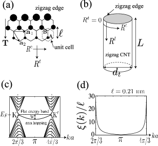
Figure 1: (a) The unit vectors of graphene are denoted by ${\bf a}_{1}$ and ${\bf a}_{2}$. ${\bf a}_{1}$ is the unit vector around the tube axis and ${\bf T}$ ($\equiv 2{\bf a}_{2}-{\bf a}_{1}$) is the translational vector along the zigzag tube axis. We define $2\ell\equiv|{\bf T}|$ where $\ell=0.21$ nm and $a\equiv|{\bf a}_{1}|$. The density of an edge state has a value only on A-atoms, which is represented by solid circles. The radius of a solid circle is proportional to the density, which shows the localization. (b) The edge states exist near the zigzag edge ($R^{t}=0$) of the $(n,0)$ CNT with open boundary. The diameter and length of the CNT is denoted by $d_{t}$ and $L$, respectively. (c) ${\cal H}_{\rm nn}$ has a flat energy band of the edge states between the K and K’ points at the Fermi energy ($E_{\rm F}=0$). ${\cal H}_{\rm nnn}$ causes a bandwidth $W=\gamma_{n}$. (d) We plot the localization length, $\xi(k)/\ell=-1/\ln(2|\cos(ka/2)|)$ for $2\pi/3<ka<4\pi/3$.

The wavefunction of the edge state is written as Sasaki et al. (2006)

$$|\Psi_{k}\rangle=\frac{N_{k}}{\sqrt{n}}\sum_{u}\exp\left\{ikR^{c}_{u,A}-\frac{R^{t}_{u,A}}{\xi(k)}\right\}|\phi({\bf R}_{u,A})\rangle,$$ (1)

where $|\phi({\bf R}_{u,s})\rangle$ is 2${\rm p}_{z}$ orbital of a carbon atom and $N_{k}$ is a normalization constant. The summation on $u$ is taken for all unit cells of graphene or a CNT. We take the coordinate ${\bf R}=(R^{c},R^{t})$ on the cylindrical surface of a zigzag CNT, in which $R^{c}$ and $R^{t}$ are coordinates around and along the tube axis, respectively (Fig. 1(b)). The position of a carbon atom is denoted by ${\bf R}_{p}\equiv(R^{c}_{u,s},R^{t}_{u,s})$ where $p=(u,s)$ represents the $s$-th sublattice ($s=A,B$) in the $u$-th hexagonal unit cell. As is taken for the zigzag edge site $R^{t}_{u,A}=0$, the edge state has amplitudes only on A-atoms ($s=A$). Equation (1) is correct for $2\pi/3<ka\leq\pi$. For $\pi<ka<4\pi/3$, a phase factor $\exp\{i\pi R^{t}_{u,A}/\ell\}$ should be multiplied to $|\phi({\bf R}_{u,A})\rangle$. Sasaki et al. (2005)

II.2 Electron-Phonon Interaction

The el-ph interaction for graphene is formulated by Jiang et al. Jiang et al. (2005), which will be applied to the edge states. The el-ph interaction for the edge states is written as

$${\cal H}_{\rm int}=\frac{1}{\sqrt{N_{\rm u}}}\sum_{k,k^{\prime}}\sum_{q_{t},\nu}\alpha^{\nu}_{kk^{\prime}}({\bf q})(b_{{\bf q},\nu}+b_{{\bf-q},\nu}^{\dagger})c_{k^{\prime}}^{\dagger}c_{k},$$ (2)

where $N_{\rm u}$ is the number of graphite unit cells, $c_{k}$ is the annihilation operator of the edge state, and $b_{{\bf q},\nu}$ is the annihilation operator of the $\nu$-th phonon mode. There are six phonon modes: out-of-plane tangential acoustic/optical mode (oTA/oTO), in-plane tangential acoustic/optical mode (iTA/iTO), and longitudinal acoustic/optical mode (LA/LO). Saito et al. (1998) $\alpha^{\nu}_{kk^{\prime}}({\bf q})$ is the el-ph interaction connecting two edge states $k$ and $k^{\prime}$ by $\nu$-th phonon mode with momentum ${\bf q}$. Due to the momentum conservation along the edge, $k^{\prime}=k+q$, while the wavevector perpendicular to the edge $q_{t}$ is needed to sum over the Brillouin zone. $\alpha^{\nu}_{kk^{\prime}}({\bf q})$ is given by $\alpha^{\nu}_{kk^{\prime}}({\bf q})\equiv A^{\nu}({\bf q})M^{\nu}_{kk^{\prime}}({\bf q})/\sqrt{2}$ where $A^{\nu}({\bf q})=\sqrt{\hbar/m_{c}\omega_{\nu}({\bf q})}$ is the amplitude of phonon ($\hbar\omega_{\nu}({\bf q})$ is the energy of the $\nu$-th phonon with the momentum ${\bf q}$) and $M^{\nu}_{kk^{\prime}}({\bf q})$ is the el-ph matrix element,

$$M^{\nu}_{kk^{\prime}}({\bf q})\equiv-\sum_{p}\langle\Psi_{k^{\prime}}|\nabla v({\bf R}_{p})|\Psi_{k}\rangle\cdot U({\bf R}_{p}){\bf e}^{\nu}_{\bf q}(s)e^{i{\bf q}\cdot{\bf R}_{p}}.$$ (3)

Here $v({\bf R}_{p})$ is the Kohn-Sham potential of a neutral pseudoatom calculated on the basis of density-functional theory by Porezag et al. Porezag et al. (1995) for a carbon atom at ${\bf R}_{p}$, ${\bf e}^{\nu}_{\bf q}(s)$ is phonon eigenvector at an $s$-atom normalized in the unit cell as $\sum_{s=A,B}{\bf e}^{\nu}_{\bf q}(s)^{*}\cdot{\bf e}^{\nu}_{\bf q}(s)=1$, and $U({\bf R}_{p})$ is a rotational operator for ${\bf e}^{\nu}_{\bf q}(s)$ from an $s$-th atom at origin to a $s$-th atom at ${\bf R}_{p}$. To obtain $\omega_{\nu}({\bf q})$ and ${\bf e}^{\nu}_{\bf q}(s)$, we use the force constant parameters calculated by Dubay and Kresse Dubay and Kresse (2003) for the dynamical matrix. Saito et al. (1998)

Putting Eq. (1) into Eq. (3), we obtain

$$M^{\nu}_{kk^{\prime}}({\bf q})=-\frac{N_{k^{\prime}}N_{k}}{n}$$

$$\times\sum_{u^{\prime},u}\exp\left\{-ik^{\prime}R^{c}_{u^{\prime},A}+ikR^{c}_{u,A}-\frac{R^{t}_{u^{\prime},A}}{\xi(k^{\prime})}-\frac{R^{t}_{u,A}}{\xi(k)}\right\}$$

$$\times m({\bf R}_{u^{\prime},A},{\bf R}_{u,A};{\bf q},\nu),$$ (4)

where $m({\bf R}_{u^{\prime},A},{\bf R}_{u,A};{\bf q},\nu)$ is the atomic deformation potential, Jiang et al. (2005) defined by

$$m({\bf R}_{u^{\prime},A},{\bf R}_{u,A};{\bf q},\nu)$$

$$\equiv\sum_{p}\langle\phi({\bf R}_{u^{\prime},A})|\nabla v({\bf R}_{p})|\phi({\bf R}_{u,A})\rangle\cdot U({\bf R}_{p}){\bf e}^{\nu}_{\bf q}(s)e^{i{\bf q}\cdot{\bf R}_{p}}.$$ (5)

There are two types of $m({\bf R}_{u^{\prime},s^{\prime}},{\bf R}_{u,s};{\bf q},\nu)$. The first type is the case of $(u^{\prime},s^{\prime})=(u,s)$ which is referred to as the on-site atomic deformation potential. Jiang et al. (2005) The other one is $(u^{\prime},s^{\prime})\neq(u,s)$ which is the off-site atomic deformation potential. The on-site (off-site) atomic deformation potential represents a scattering process of an electron from ${\bf R}_{u,s}$ to the same (different) site.

The off-site deformation potential matrix element for the next-nearest A atoms, $|\langle\phi({\bf R}_{u^{\prime},A})|\nabla v({\bf R}_{p})|\phi({\bf R}_{u,A})\rangle\cdot{\hat{n}}|$, is negligible (for any ${\bf R}_{p}$) in Eq. (5) because it decay quickly as a function of $|{\bf R}_{u^{\prime},A}-{\bf R}_{u^{\prime},A}|$ where ${\hat{n}}$ is a unit vector along the two carbon atoms. Density-functional theory gives that the off-site deformation potential matrix element for nearest-neighbor interaction is $|\langle\phi({\bf R}_{u,B})|\nabla v({\bf R}_{u,B})|\phi({\bf R}_{u,A})\rangle\cdot{\hat{n}}|\sim$ 3eV/Å. Jiang et al. (2005); Porezag et al. (1995) As we pointed out above, the wavefunction of the edge state has an amplitude only of one sublattice and thus this nearest-neighbor term does not contribute to $\alpha^{\nu}_{kk^{\prime}}({\bf q})$. Thus the off-site atomic deformation potential does not contribute to $\alpha^{\nu}_{kk^{\prime}}({\bf q})$ for the edge states. For the on-site atomic deformation potential, we need to consider several carbon atoms which are located near ${\bf R}_{u,A}$ for the center of deformation potential ${\bf R}_{p}$ in Eq. (5). The value of $|\langle\phi({\bf R}_{u,A})|\nabla v({\bf R}_{p})|\phi({\bf R}_{u,A})\rangle\cdot{\hat{n}}|$ is not negligible if $|{\bf R}_{p}-{\bf R}_{u,A}|\leq 3$Å. Density-functional theory gives that the largest contribution from nearest-neighbor site is $|\langle\phi({\bf R}_{u,A})|\nabla v({\bf R}_{u,B})|\phi({\bf R}_{u,A})\rangle\cdot{\hat{n}}|\sim 8$ eV/Å. Porezag et al. (1995) Thus on-site deformation potential is more important than the off-site deformation potential. Suzuura and Ando (2002)

Now we can write $m({\bf R}_{u^{\prime},A},{\bf R}_{u,A};{\bf q},\nu)$ as

$$m({\bf R}_{u^{\prime},A},{\bf R}_{u,A};{\bf q},\nu)=\delta_{u^{\prime}u}m_{\rm on}(R_{u,A}^{t};{\bf q},\nu)e^{i{\bf q}\cdot{\bf R}_{u,A}},$$ (6)

where $m_{\rm on}(R_{u,A}^{t};{\bf q},\nu)$ is on-site deformation potential from all possible ${\bf R}_{p}$, defined as

$$m_{\rm on}(R_{u,A}^{t};{\bf q},\nu)\equiv$$

$$\sum_{p}\langle\phi({\bf R}_{u,A})|\nabla v({\bf R}_{p})|\phi({\bf R}_{u,A})\rangle\cdot U({\bf R}_{p}){\bf e}^{\nu}_{\bf q}(s)e^{i{\bf q}\cdot({\bf R}_{p}-{\bf R}_{u,A})}.$$ (7)

Putting Eq. (6) into Eq. (4), we get

$$M^{\nu}_{kk^{\prime}}({\bf q})=-N_{k^{\prime}}N_{k}\delta_{k^{\prime},k+q}$$

$$\sum_{R_{u,A}^{t}}\exp\left\{\left(iq_{t}-\frac{1}{\xi(k^{\prime})}-\frac{1}{\xi(k)}\right)R^{t}_{u,A}\right\}m_{\rm on}(R_{u,A}^{t};{\bf q},\nu).$$ (8)

For $ka\leq\pi<k^{\prime}a$ or $k^{\prime}a\leq\pi<ka$, we must multiply $\exp\{i\pi R^{t}_{u,A}/\ell\}$ to $m_{\rm on}(R_{u,A}^{t};{\bf q},\nu)$ in Eq. (8).

It is noted that $m_{\rm on}(R_{u,A}^{t};{\bf q},\nu)$ is defined to be independent of $R^{c}_{u,A}$. Instead, $R^{c}_{u,A}$ appears in the phase of $m({\bf R}_{u,A},{\bf R}_{u,A};{\bf q},\nu)$ in Eq. (6). The phase gives the momentum conservation around the tube axis, $\delta_{k^{\prime},k+q}$, after the summation about $R_{u,A}^{c}$ is made in Eq. (4). On the other hand, $m_{\rm on}(R_{u,A}^{t};{\bf q},\nu)$ depends on $R_{u,A}^{t}$ because $\sum_{p}$ in Eq. (7) is restricted for $R^{t}_{p}\geq 0$ and $m_{\rm on}(R_{u,A}^{t};{\bf q},\nu)$ does not have a translational symmetry near the edge. Hereafter, we refer $m_{\rm on}(R_{u,A}^{t};{\bf q},\nu)$ as boundary deformation potential.

$m_{\rm on}(R_{u,A}^{t};{\bf q},\nu)$ depends on $\nu$ strongly. The iTO and LO modes whose eigenvectors are pointing in the direction perpendicular to the edge give a large contribution to $m_{\rm on}(R_{u,A}^{t};{\bf q},\nu)$. We generally expect that the boundary deformation potential appears only near the edge. In fact, $|\langle\phi({\bf R}_{u,A})|\nabla v({\bf R}_{p})|\phi({\bf R}_{u,A})\rangle\cdot{\hat{n}}|$ is finite only when $|{\bf R}_{p}-{\bf R}_{u,A}|\leq 3$Å. Thus $m_{\rm on}(R_{u,A}^{t};{\bf q},\nu)$ depends on $R^{t}_{u,A}$ only when $R^{t}_{u,A}\leq 3$Å. The boundary deformation potential contributes to the matrix element increasingly with decreasing $\xi(k)$ or $\xi(k^{\prime})$, which can be seen in Eq. (8).

In Eq. (7), we must consider relative atomic motion of ${\bf R}_{u,A}$ to ${\bf R}_{p}$. This can be done by replacing $U({\bf R}_{p})$ with $U({\bf R}_{p})-E$ where $E$ is the unit matrix. In Fig. 2(a) we show phonon eigenvector of the oTA mode pointing perpendicular to the nanotube surface. If we consider the phonon eigenvector in a flat surface or graphene, the relative displacement of the two atoms becomes zero when ${\bf q}={\bf 0}$. However, it is not the case for a cylindrical surface. As shown in Fig. 2(b), the relative eigenvector, $(U({\bf R}_{p})-E){\bf e}^{\rm oTA}_{\bf q}(s)$, remains finite. The relative vector for the oTA mode changes the area on a cylindrical surface and is similar to the LA mode except for a $1/d_{t}$ reduction of the amplitude, by which $m_{\rm on}(R_{u,A}^{t};{\bf q},{\rm oTA})$ is proportional to $1/d_{t}$. On the other hand, the relative displacement becomes zero for the in-plane modes such as iTA and LA, when ${\bf q}\to{\bf 0}$. Thus, the el-ph interaction by the iTA and LA modes vanish for ${\bf q}={\bf 0}$ while the oTA mode provides a finite $m_{\rm on}(R_{u,A}^{t};{\bf q},{\rm oTA})$ even for ${\bf q}={\bf 0}$. Hereafter, we simply use $U({\bf R}_{p})$ for $U({\bf R}_{p})-E$.

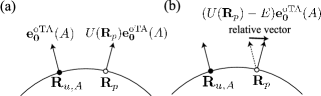
Figure 2: (a) For the oTA mode with ${\bf q}={\bf 0}$, the eigenvectors of two atoms at ${\bf R}_{u,A}$ and ${\bf R}_{p}$ are pointing perpendicular to the CNT surface. (b) In order to calculate the atomic deformation potential, one needs to consider the relative displacement of two carbon atoms.

III Calculated Results

In this section, we plot $|M_{kk^{\prime}}^{\nu}({\bf q})|$ for several values of $k$ and $k^{\prime}$, and examine the dependence of $|M_{kk^{\prime}}^{\nu}({\bf q})|$ on phonon mode $\nu$ in Sec. III.0.1 and on nanotube diameter $d_{t}$ in Sec. III.0.2.

III.0.1 $\nu$ dependence of $|M_{kk^{\prime}}^{\nu}({\bf q})|$

In the calculation, we consider the magnitude of $M_{kk^{\prime}}^{\nu}({\bf q})$ for the $(60,0)$ CNT ($d_{t}\approx 5$ nm). In Fig. 3, we plot $|M_{kk^{\prime}}^{\nu}({\bf q})|$ as a function of $q_{t}$ for (a) $(k,k^{\prime})=(7\pi/10,8\pi/10)$ and (b) $(26\pi/30,29\pi/30)$. The corresponding phonon eigenvector is the same ($q=\pi/10$). Thus the difference between the two cases shows the dependence of $|M_{kk^{\prime}}^{\nu}({\bf q})|$ on $\xi(k)$ and $\xi(k^{\prime})$. $(7\pi/10,8\pi/10)$ is chosen as an example that $\xi(k)$ ($=22$Å) and $\xi(k^{\prime})$ ($=4.4$Å) are longer than the carbon-carbon bond length ($a_{\rm cc}=1.4$Å), while $(26\pi/30,29\pi/30)$ is chosen as an example that $\xi(k)$ ($=2.4$Å) and $\xi(k^{\prime})$ ($=0.9$Å) are comparable to $a_{\rm cc}$.

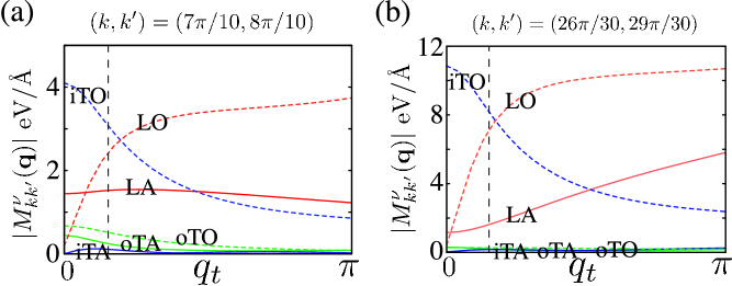
Figure 3: (Color online) $|M_{kk^{\prime}}^{\nu}({\bf q})|$ for the $(60,0)$ zigzag CNT: (a) $(k,k^{\prime})=(7\pi/10,8\pi/10)$ and (b) $(k,k^{\prime})=(26\pi/30,29\pi/30)$ are plotted as a function of $q_{t}$ where $q=\pi/10$. Three solid curves represent acoustic phonon modes: oTA(green), iTA(blue) and LA (red), and three dashed curves are optical modes: oTO(green), iTO(blue) and LO (red). The vertical dashed lines represent $q_{t}=\sqrt{3}q$ ($\sqrt{3}=|{\bf T}|/|{\bf a}_{1}|$).

As shown in Fig. 3(a), $|M_{kk^{\prime}}^{\rm iTO}({\bf q})|$ is 4 eV/Å at $q_{t}=0$. $|M_{kk^{\prime}}^{\rm iTO}({\bf q})|$ decreases with increasing $q_{t}$, while $|M_{kk^{\prime}}^{\rm LO}({\bf q})|$ increases with increasing $q_{t}$. This behavior of the iTO and LO modes relates to the boundary deformation potential. The eigenvector of the iTO (LO) mode is pointing along the tube axis when $q_{t}/|{\bf T}|<q/|{\bf a}_{1}|$ ($q_{t}/|{\bf T}|>q/|{\bf a}_{1}|$) and then produces a large boundary deformation potential. On the other hand, ${\bf e}^{\rm oTO}_{\bf q}(s)$ is perpendicular to the CNT axis and the oTO mode does not contribute to a boundary deformation potential. The value of $|M_{kk^{\prime}}^{\rm oTO}({\bf q})|$ is considerably smaller than $|M_{kk^{\prime}}^{\nu}({\bf q})|$ for the iTO and LO modes. Thus the contribution of the oTO mode to the el-ph interaction can be neglected for $d_{t}\approx 5$ nm CNT. In Fig. 3(b), $|M_{kk^{\prime}}^{\rm iTO}({\bf q})|$ and $|M_{kk^{\prime}}^{\rm LO}({\bf q})|$ reach 11 eV/Å, which indicates that $|M_{kk^{\prime}}^{\nu}({\bf q})|$ for the iTO and LO modes increase significantly with decreasing $\xi(k)$ and $\xi(k^{\prime})$. The boundary deformation potential becomes more effective with decreasing the localization length.

The matrix element for iTA mode is smaller than the other acoustic modes for a wide range of $q_{t}$ as shown in Fig. 3(a). Though $|M_{kk^{\prime}}^{\rm iTA}({\bf q})|$ can be comparable to $|M_{kk^{\prime}}^{\rm oTA}({\bf q})|$ as shown in Fig. 3(b), the contribution of the iTA mode to the el-ph interaction is negligible to that for oTA because the amplitude of the iTA mode is smaller than that of the oTA mode; $A^{\rm iTA}({\bf q})\lesssim A^{\rm oTA}({\bf q})$. On the other hand, the oTA and LA modes are important for lower temperature in the el-ph interaction. The oTA mode changes the volume of a CNT and gives an on-site deformation potential as shown in Fig. 2. Moreover, the energy of the oTA mode is smallest among acoustic modes and thus $A^{\rm oTA}({\bf q})$ can be larger than $A^{\rm LA}({\bf q})$. The LA mode is a area-changing mode and produces a large on-site deformation potential, and contributes to the matrix element most significantly among acoustic modes.

III.0.2 $d_{t}$ dependence of $|M_{kk^{\prime}}^{\nu}({\bf q})|$

It is shown from Eq. (8) that $M_{kk^{\prime}}^{\nu}({\bf q})$ for two CNTs with different diameters ($d_{t}$) are the same for the same values of $k$ and $k^{\prime}$. In general, we can find the similar values of $k$ (or $k^{\prime}$) for different $d_{t}$. However, it is not the case for edge states near the K or K’ point. Then $M_{kk^{\prime}}^{\nu}({\bf q})$ depends on $d_{t}$ for such edge states. For instance, $M_{kk^{\prime}}^{\nu}({\bf q})$ depends on $d_{t}$ for the largest $\xi(k)\approx d_{t}/2$. In Fig. 4, we plot $|M_{kk^{\prime}}^{\nu}({\bf q})|$ for $(41\pi/60,47\pi/60)$ of the $(120,0)$ CNT ($d_{t}\approx 10$ nm). $|M_{kk^{\prime}}^{\nu}({\bf q})|$ has the similar functional shape as shown in Fig. 3(a) while the values become smaller.

The reduction of $|M_{kk^{\prime}}^{\nu}({\bf q})|$ can be explained as follows. If we neglect $d_{t}$ dependence of the boundary deformation potential, the summation on $R^{t}_{u,A}$ in Eq. (8) can be performed analytically. $M_{kk^{\prime}}^{\nu}(q_{t}=0)$ is then proportional to the factor $R_{kk^{\prime}}(d_{t})$;

$$R_{kk^{\prime}}(d_{t})\equiv\frac{\sqrt{\xi(k)\xi(k^{\prime})}}{\xi(k)+\xi(k^{\prime})},$$ (9)

where $R_{kk^{\prime}}(d_{t})$ is a function of $d_{t}$ because $\xi$ depends on $d_{t}$. Since $R_{kk^{\prime}}(5{\rm nm})=0.37$ and $R_{kk^{\prime}}(10{\rm nm})=0.30$, we have $R_{kk^{\prime}}(10{\rm nm})/R_{kk^{\prime}}(5{\rm nm})\approx 0.81$. This ratio reproduces $|M_{kk^{\prime}}^{\rm LA}({\bf q})|_{10{\rm nm}}/|M_{kk^{\prime}}^{\rm LA}({\bf q})|_{5{\rm nm}}=1.3/1.5\approx 0.86$ at $q_{t}=0$.

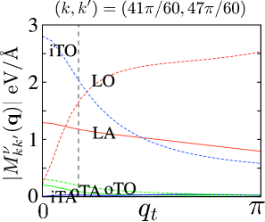
Figure 4: (Color online) $|M_{kk^{\prime}}^{\nu}({\bf q})|$ for $(120,0)$ zigzag CNT. The phonon eigenvector is the same as Fig. 3. The vertical dashed line represents $q_{t}=\sqrt{3}q$.

IV Local density of states

Now we calculate a renormalized energy dispersion relation and LDOS using self-energy $\Sigma(k,i\omega_{n})$ which is defined by

$$\Sigma(k,i\omega_{n}) =\frac{2k_{\rm B}T}{N_{\rm u}}\sum_{m}\sum_{{\bf q},\nu}\frac{|\alpha_{kk+q}^{\nu}({\bf q})|^{2}\hbar\omega_{\nu}({\bf q})}{(\omega_{n}-\omega_{m})^{2}+(\hbar\omega_{\nu}({\bf q}))^{2}}$$

$$\times\frac{1}{i\omega_{m}-(E(k+q)-E_{\rm F})-\Sigma(k+q,i\omega_{m})},$$ (10)

where $T$ is temperature and $\omega_{n}=\pi k_{\rm B}T(2n+1)$ is the Matsubara frequency ($n$ is integer). We put the cut-off Matsubara frequency, $|\omega_{n}|\leq\hbar\omega_{\rm D}\approx 0.2$ eV. By means of Padé approximation, Vidberg and Serene (1977) $\Sigma(k,i\omega_{n})$ is changed to that on the real-axis of $\omega$: $\Sigma(k,\omega)$. Then we find a solution $\epsilon$ satisfying $\epsilon=(E(k)-E_{\rm F})+{\rm Re}\left(\Sigma(k,\epsilon)\right)$ as a function of $k$, $E_{\rm F}$ and $T$. The obtained $\epsilon_{E_{\rm F},T}(k)$ is a renormalized energy dispersion relation. We adopt $T=50$ K in the following calculations. The $T$-dependence of $\epsilon_{E_{\rm F},T}(k)$ is negligible for a wide range of $T$, for instance, $T=77$ K gives almost the same result. Calculations at low temperature have some numerical advantage since the number of $\omega_{n}$ increases. The LDOS curve is defined as a function of bias voltage ($V$) between graphene and the STS tip, and the distance ($R^{t}$) from the zigzag edge sites and the STS tip by

$$D(V,R^{t})=\frac{1}{\pi}\sum_{k}\frac{\Gamma_{E_{\rm F}}(k)}{(V-\epsilon_{E_{\rm F}}(k))^{2}+\Gamma_{E_{\rm F}}(k)^{2}}|\Psi_{k}(R^{t})|^{2},$$ (11)

where $\Gamma_{E_{\rm F}}(k)\equiv-2{\rm Im}(\Sigma(k,\epsilon_{E_{\rm F}}(k)))$ is the width of STS spectrum. It is noted that the value of $E_{\rm F}$ is given in such a way that the number of valence (edge) states is conserved when we calculate $\Sigma(k,i\omega_{n})$ self-consistently, that is, $\sum_{E(k)<E_{\rm F}}1=\sum_{\epsilon_{E_{\rm F}}(k)<E_{\rm F}}1$.

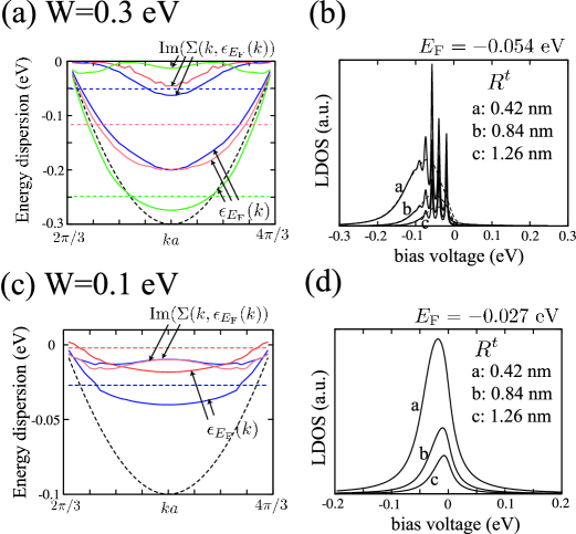
Figure 5: (Color online) Calculated energy dispersion $\epsilon_{E_{\rm F}}(k)$ and LDOS $D(V,R^{t})$ for (a,b) $W=0.3$ eV and (c,d) $W=0.1$ eV. In (a), $E(k)$ is plotted as the dashed curve, and $\epsilon_{E_{\rm F}}(k)$ is plotted for $E_{\rm F}=-0.054$, $-0.122$, $-0.250$ eV. We plot ${\rm Im}(\Sigma(k,\epsilon_{E_{\rm F}}(k)))$ to show the $k$-dependence. In (b), $D(V,R^{t})$ for $E_{\rm F}=-0.054$ eV and its smoothed curve (dashed curve) are plotted for $R^{t}=0.42$, $0.84$ and $1.26$ nm. In (c), $\epsilon_{E_{\rm F}}(k)$ is plotted for $E_{\rm F}=-0.002$ eV and $-0.027$ eV. In (d), we plot $D(V,R^{t})$ for $E_{\rm F}=-0.027$ eV.

IV.1 Numerical Result

In Fig. 5(a), we plot $E(k)$ ($W=0.3$ eV) without self-energy correction as the dashed curve and renormalized energy dispersion $\epsilon_{E_{\rm F}}(k)$ for $E_{\rm F}=-0.054$, $-0.122$, $-0.250$ eV as the blue, red and green curves, respectively. The reason why we consider different $E_{\rm F}$ values is that in the experiment charge transfer from STS tip or substrate may modify the $E_{\rm F}$ values and that we need to investigate $E_{\rm F}$ dependence. The parallel dashed lines denote the Fermi level for these $E_{\rm F}$ values. For each value of $E_{\rm F}$, ${\rm Im}(\Sigma(k,\epsilon_{E_{\rm F}}(k)))$ is plotted to show the $k$-dependence. By denoting the renormalized bandwidth as $W^{\prime}$, we obtain $W^{\prime}\approx 0.2$ eV for $E_{\rm F}=-0.054$ eV and $-0.122$ eV. The corresponding mass enhancement parameter $\lambda$ is about 0.5 where we defined $\lambda=W/W^{\prime}-1$. When $E_{\rm F}=-0.250$ eV, $W^{\prime}$ is about 0.27 eV and $\lambda\approx 0.1$. We observe that the value of $\Gamma_{E_{\rm F}}(k=\pi)$ is about 0.13 eV when $E_{\rm F}=-0.054$ eV. The calculated $\epsilon_{E_{\rm F}}(k)$ and ${\rm Im}(\Sigma(k,\epsilon_{E_{\rm F}}(k)))$ strongly depend on the value of $E_{\rm F}$.

The values of $W^{\prime}$ and $\Gamma_{E_{\rm F}}(k)$ relate to the peak position and width of $D(V,R^{t})$. We plot $D(V,R^{t})$ for $E_{\rm F}=-0.054$ eV at $R^{t}=0.42$, $0.84$, $1.26$ nm in Fig. 5(b). The LDOS curves have several sharp spikes at $V=\epsilon_{E_{\rm F}}(k)$ due to relatively small value of $\Gamma_{E_{\rm F}}(k)$ compared with the finite level spacing of the edge states. Here we take $(120,0)$ CNT ($d_{t}\approx 10$ nm) for calculating the self-energy. For a graphene ($d_{t}\to\infty$), the level spacing becomes zero and the spike structure will disappear. The calculated LDOS structure for $E_{\rm F}=-0.054$ eV has a peak near $V\approx-60$ meV which is close to the observed LDOS in which a peak is located at $V=-30\sim-20$ meV. Niimi et al. (2005, 2006); Kobayashi et al. (2005, 2006) However, the width of the peak is about 0.7 eV, which is much larger than the experiment Niimi et al. (2005); Kobayashi et al. (2005) ($0.05\sim 0.1$ eV). The peak position and the width are improved to fit the experimental data when $W=0.1$ eV as shown in Fig. 5(c) and (d). In this case, $W^{\prime}=0.02$ and $0.04$ for $E_{\rm F}=-0.002$ and $-0.27$ eV, respectively. The calculated LDOS structure for $E_{\rm F}=-0.027$ eV has a peak near $V\approx-20$ meV with the width of $\approx 0.05$ eV. The small value of $W$ does not show any spike structure due to the discrete $k$ values. Thus overall feature seems to be better for $W=0.1$ eV than $W=0.3$ eV. It should be noted that $W=0.1$ eV is not always consistent to the experiment. When we assume all the edge states are below the Fermi energy, we see that $E_{\rm F}$ appears above $E=0$ eV which gives a peak very close or above the $V=0$ eV, while the experiment shows $V=-30\sim-20$ meV.

It is worth mentioning that Niimi et al. Niimi et al. (2005, 2006) reported that the tunnel current was unstable when the STS tip was located very close to the zigzag edge. Then the electron injected from the STS tip has a large transition amplitude to edge states having $\xi(k)<2\ell$ (0.42 nm), that is, $k$-states which are around $k=\pi$ state (see Fig. 1(d)). As shown in Fig. 5(c), the magnitude of $\Gamma_{E_{\rm F}}(k)$ is much larger than $k_{\rm B}T$ ($\approx$ 0.0045eV) for most value of $k$ and $\Gamma_{E_{\rm F}}(k)$ for states around $k=\pi$ state reaches about 0.02 eV and yield strong fluctuation. It indicates that the tunnel current is unstable. We calculate $D(V,0)$ and find that the height and width of the peak are both significantly larger (more than 10 times larger) than $D(V,R^{t})$ for $R^{t}=0.42$ nm. As we noted in Sec. II, iTO and LO modes give a large matrix element through the boundary deformation potential. The boundary deformation potential may be relevant to the unstable tunnel current. Since the injected electron from a STS tip is localized near the edge, we expect that the tunnel current would be strongly affected by the boundary deformation potential.

V discussion and summary

We showed that el-ph interaction for edge states consists only of the on-site atomic deformation potential. As a result, LA mode contributes to scattering most effectively and the on-site deformation potential is enhanced at the edge for LO and iTO modes. It is to be noted that the on-site atomic deformation potential does not contribute to backward scattering of extended states and the off-site atomic deformation potential gives rise to resistivity. Suzuura and Ando (2002) Because the on-site atomic deformation potential is larger than the off-site atomic deformation potential, the edge states exhibit the strong el-ph coupling character that the graphite system originally possesses.

The original energy bandwidth of the edge states, $W$, is consistent with the observed position of LDOS peak when $W\approx 0.1$ eV, which is the same order of $\gamma_{n}\approx 0.3$ eV but not the same value. It is noted that the case of $W=0.3$ eV does not include the overlapping integral ($s$ parameter Saito et al. (1998)) which increases (decreases) the conduction (valence) bandwidth. To examine the effect of $s$ parameter on the bandwidth of the edge states, we performed the energy band structure calculation in an extended tight-binding framework Samsonidze et al. (2004) and obtained $W\approx 0.2$ eV. We expect that $W$ is externally modified by attaching a functional group or contacting an electrode to the edge sites. In addition to the el-ph interaction, electron-electron (el-el) interaction causes self-energy which may account for the difference. The el-el interaction contributes to $\Sigma(k,i\omega_{n})$ additively when there is no cross term of el-ph and el-el interactions. Since many papers report the importance of el-el interaction, especially the contribution to the imaginary part of self-energy should be important and thus the spike structure of discrete $k$ does not appear in the real case. Then $W^{\prime}$ decreases and the width of LDOS increases. The effect of el-el interaction warrants future work concerning the effects of dynamical details on LDOS curve. A detail experimental data of STM/STS for zigzag edge of CNTs and graphene may be useful for a qualitative estimation of the strength of the el-el interaction. When the values of $W$ and $\hbar\omega_{\rm D}$ are comparable, the vertex correction may be important since the Migdal theorem is not applicable. Although our results are consistent with the STS data, it is possible that vertex correction may change $\alpha_{kk^{\prime}}^{\nu}({\bf q})$. However the vertex correction to $\alpha^{\nu}_{kk^{\prime}}({\bf q})$ is beyond our scope in the present paper.

We did not consider the el-ph matrix element between extended state and edge state. Although the matrix element may be enhanced by the boundary deformation potential, it is naively expected that the matrix element is proportional to $\sqrt{\xi/L}$ and is negligible when $L\gg\xi$. In this case, the extended state and the edge state can be decoupled. The geometry with $d_{t}\gg L$ is referred to as the nano-graphite ribbon. For a ribbon, the off-site atomic deformation potential contributes to the scattering between two edge states which are located at the different edges since overlapping between the two edge states is not negligible. It is noted that Igami et al. Igami et al. (1998) showed that out-of-plane edge phonon modes appear depending on the effective mass of carbon atom at edge sites, and Tanaka et al. Tanaka et al. (2002) observed such modes at the armchair edge of nano-graphite ribbons on TiC(755) surface by high resolution electron energy loss spectroscopy. Though ${\bf e}^{\nu}_{\bf q}(s)$ and $\omega_{\nu}({\bf q})$ used in this paper do not include the edge phonon mode, el-ph coupling for out-of-plane modes is negligible for the edge states. The el-ph interaction for nano-ribbon requires further studies on the el-ph interaction.

In summary, we formulated el-ph interaction for edge states and used it to calculate LDOS. Although our calculation does not include the Coulomb interaction, the result agrees with LDOS data Niimi et al. (2005, 2006); Kobayashi et al. (2005) when $W\approx 0.1$ eV. Our results should be compared with the future experiments of edge states in CNTs and graphene.