Coherence and Entanglement in Two-Qubit Dynamics: Interplay of the Induced Exchange Interaction and Quantum Noise due to Thermal Bosonic Environment

Abstract

We present a review of our recent results for the comparative evaluation of the induced exchange interaction and quantum noise mediated by the bosonic environment in two-qubit systems. We report new calculations for P-donor-electron spins in Si-Ge type materials. Challenges and open problems are discussed.

Keywords: decoherence, entanglement, qubit, exchange interaction, quantum noise, quantum computing.

.  

1 INTRODUCTION

In this review we present results of our recent investigations[1, 2] addressing several problems in the field of open quantum systems; some have a rather long history. With the actual experimental probes now being carried out at the nanoscale, these problems have become more pressing, and some have actually been suggested by the experimental developments.[3, 4, 5, 6, 7, 8, 9, 10, 11, 12, 13, 14] Perhaps the most fundamental (and difficult) of these problems is the matter of accounting within a calculationally tractable approach for relaxation vs. coherent dynamics in open quantum systems. In particular the coherent and quantum-noise features induced by the bosonic environment (bath of noninteracting bosonic modes) are especially interesting, because this model is widely applicable for quantum computing systems. Here we consider bath-induced RKKY-type exchange interactions in two-qubit systems.

This paper is organized as follows. In the next section, Sec. 2, we formulate the model and discuss the issue of the initial conditions. An example of the semiconductor (Si-Ge type) based qubit model is given and the nature of the interactions is discussed.

Section 3 is devoted to the initial dynamics of the induced interaction and quantum noise. In particular, in Sec. 3.1 we present an exactly solvable model to obtain the exchange interaction as well as the time-dependent correction due to the initial conditions. The model also demonstrates the delay in the response of the qubits caused by the finite propagation velocities of the mediating virtual bosons. In Sec. 3.2, we study the interplay of the coherent dynamics and quantum noise by calculating the concurrence.[15, 16] Evolution of the reduced density matrix elements is also investigated.

At large times, as the system forgets the initial state, the exchange interaction becomes stationary. This regime is discussed in Sec. 4. We utilize the master-equation formulation of Markovian dynamics, Sec. 4.1, and go over an illustrative one-dimensional (1D) example of the emerging interaction and quantum noise in Sec. 4.2. Generalization to higher dimensionality is given in Sec. 4.3. A solid-state based three-dimensional (3D) example of a semiconductor qubit model is presented in Sec. 4.4. In the latter discussion we compare bath-induced coupling and noise to other interactions, such as an electromagnetic coupling of P-impurity spins (qubits). Finally, brief summary and outline of some open challenges are offered in Sec. 5.

A

2 THE MODEL AND INITIAL CONDITIONS

We consider two qubits, i.e., two two-state quantum systems, modeled by localized electron spins ($1/2$) immersed in a common quantum environment. The qubits are located at the distance $\mathbf{d}$ from each other, far enough so that the direct overlap of the electron wave functions is negligible. The environment is modeled by a bath of bosonic modes, which are maintained at temperature $T$. It is usually assumed that external influences, as well as possibly internal bath-mode interactions, set a fast time scale $t_{B}$ for the bath correlations to equilibrate. The bath modes are then regarded as otherwise noninteracting. At least for the low-frequency bath modes, it is usually argued that such a thermalization time for a generic case should be of order $\hbar/k_{\textrm{B}}T$. The thermal-state density matrix of the bath modes, taken here as noninteracting bosonic fields, is

$$\rho_{B}=\mathrm{Z}^{-1}\exp\bigg{[}{-{\sum\limits_{\mathbf{k},\mathbf{\xi}}{\omega_{\mathbf{k},\mathbf{\xi}}a_{\mathbf{k},\mathbf{\xi}}^{\dagger}a_{\mathbf{k},\mathbf{\xi}}}}/{k_{\textrm{B}}T}}\bigg{]}\,,$$ (1)

where we set $\hbar=1$, and the partition function is $\mathrm{Z}=1/\prod_{k}(1-e^{-\omega_{k}/k_{\textrm{B}}T})$. The bath is linearly coupled to each qubit,

$$H_{SB}=\sum\limits_{j=1,2}\sum\limits_{m=x,y,z}\sigma^{j}_{m}X^{j}_{m}\,,$$ (2)

where the superscripts ($j=1,2$) label the two spins, and the bath operators are given by

$$X^{j}_{m}=\sum_{\mathbf{k},\mathbf{\xi}}g^{m}_{\mathbf{k},\mathbf{\xi}}e^{i\mathbf{k}\cdot\mathbf{r}_{j}}\left(a_{\mathbf{k},\mathbf{\xi}}+a_{-\mathbf{k},\mathbf{\xi}}^{\dagger}\right)\,.$$ (3)

The overall Hamiltonian of the qubit-bath system is

$$H=H_{S}+H_{B}+H_{SB}\,,$$ (4)

where

$$H_{B}=\sum_{\mathbf{k},\mathbf{\xi}}\omega_{\mathbf{k},\mathbf{\xi}}a_{\mathbf{k},\mathbf{\xi}}^{\dagger}a_{\mathbf{k},\mathbf{\xi}}\,,$$ (5)

and the two spin-$1/2$ (qubits) will be assumed split by external magnetic field,

$$H_{S}=\Delta(\sigma_{z}^{1}+\sigma_{z}^{2})/2\,.$$ (6)

Here $\Delta$ is the energy gap between the up and down states for spins 1 and 2. A natural example of such a system are spins of two localized electrons interacting via lattice vibrations (phonons) by means of the spin-orbit interaction.[17, 18, 19, 20] Another example is provided by atoms or ions in a cavity, used as two-state systems interacting with photons.[21]

Our emphasis here will be on calculating and comparing the relative importance of the coherent (induced interaction) vs. quantum-noise effects of a given bosonic bath in the two-qubit dynamics. We do not include other possible two-qubit interactions in such comparative calculation of dynamical quantities. In Sec. 4.4 we also include the direct electromagnetic (EM) coupling for a comparison of the bath-induced and EM dipole-dipole interaction strengths.

An interesting realization of the model formulated above can be found in the impurity electron spin dynamics in semiconductors. Let us consider P donor impurities embedded at controlled positions in an otherwise very clean Si (or Ge) crystal matrix. The system is maintained at very low temperature, as appropriate for quantum computing. Therefore, the outer donor-impurity electron remains bound. The spins of such localized electrons can be utilized as qubits. They are subject to external magnetic field $\mathbf{H}$, which produces the Zeeman splitting (6). The spin-orbit interaction couples the spin to the deformation potential fluctuations of the host semiconductor, producing the energy change

$$H_{\textrm{SO}}=\mu_{\textrm{B}}\!\!\sum\limits_{m,l\,=\,x,y,z}\!\!{\sigma_{m}g_{ml}H_{l}}\,,$$ (7)

where $\mu_{\textrm{B}}$ is the Bohr magneton, and $\mathbf{H}=\{H_{x},H_{y},H_{z}\}$. Here the tensor $g_{ml}$ is sensitive to lattice deformations. It was shown[19] that for the donor state which has tetrahedral symmetry (which is the case for P in Si or Ge), the Hamiltonian (7) yields the spin-deformation interaction of the form

$$H_{i}={\rm A}\mu_{\textrm{B}}\left[{\bar{\varepsilon}_{xx}\sigma_{x}H_{x}+\bar{\varepsilon}_{yy}\sigma_{y}H_{y}+\bar{\varepsilon}_{zz}\sigma_{z}H_{z}+{\bar{\Delta}}(\mathbf{\sigma}\cdot\mathbf{H}})/3\right]\\ +\,{\rm B}\mu_{\textrm{B}}\left[{\bar{\varepsilon}_{xy}\left({\sigma_{x}H_{y}+\sigma_{y}H_{x}}\right)+{\text{c}}{\text{.p}}{\text{.}}}\right]\,.$$ (8)

Here c.p. denotes cyclic permutations and $\bar{\Delta}$ is the effective dilatation. The tensor $\bar{\varepsilon}_{ij}$ already includes averaging of the strain with the gradient of the potential over the donor ground state wave function.

As before, let us assume that we have two impurities separated by distance d. For definiteness, one can direct the magnetic field along the $z$-axis. Then the spin-deformation interaction Hamiltonian simplifies to

$$H_{i}={\rm A}\mu_{\textrm{B}}\bar{\varepsilon}_{zz}\sigma_{z}^{i}H_{z}+{\rm B}\mu_{\textrm{B}}\left({\bar{\varepsilon}_{yz}\sigma_{y}^{i}H_{z}+\bar{\varepsilon}_{zx}\sigma_{x}^{i}H_{z}}\right)\,.$$ (9)

In terms of the quantized phonon field, we have[17, 22]

$$\bar{\varepsilon}_{ij}=\sum\limits_{{\mathbf{k}},{\mathbf{\xi}}}{f({\mathbf{k}})\sqrt{\frac{\hbar}{{8\rho V\omega_{{\mathbf{k}},{\mathbf{\xi}}}}}}\left({\xi_{{\mathbf{k}},i}k_{j}+\xi_{{\mathbf{k}},j}k_{i}}\right)\left({a_{{\mathbf{k}},{\mathbf{\xi}}}^{\dagger}+a_{{\mathbf{k}},{\mathbf{\xi}}}}\right)}\,,$$ (10)

where in the spherical donor ground state approximation[18, 22]

$$f({\mathbf{k}})=\frac{1}{{\left({1+a_{\textrm{B}}^{2}k^{2}}\right)^{2}}}\,.$$ (11)

Here $a_{\textrm{B}}$ is half the effective Bohr radius of the donor ground state wave function. In an actual Si or Ge crystal, donor states are more complicated and include corrections due to the symmetry of the crystal matrix including the fast Bloch-function oscillations. However, the wave function of the donor electrons in our case is spread over several atomic dimensions (see below). Therefore, it suffices to consider “envelope” quantities. Thus, in the spin-phonon Hamiltonian (2)-(3) coupling constants will be taken in the form

$$g_{{\mathbf{k}},{\mathbf{\xi}}}^{m}=\frac{D_{m}}{{\left({1+a_{\textrm{B}}^{2}k^{2}}\right)^{2}}}\sqrt{\frac{\hbar}{{8\rho V\omega_{{\mathbf{k}},{\mathbf{\xi}}}}}}\left({\xi_{{\mathbf{k}},z}k_{m}+\xi_{{\mathbf{k}},m}k_{z}}\right)\,,$$ (12)

where $D_{x}=D_{y}={\rm B}\mu_{\textrm{B}}H_{z}$ and $D_{z}={\rm A}\mu_{\textrm{B}}H_{z}$.

It will be instructive to consider a one-dimensional calculation, which simplifies the notation. General results[1, 2] are presented later in this article. One can think of a 1D channel geometry along the $z$ direction. This will give an example of an Ohmic bath model discussed later. In a 1D channel the boundaries[23] can approximately quantize the spectrum of the phonons along $x$ and $y$, depleting the density of states except at certain resonant values. Therefore, the low-frequency effects, including the induced coupling and quantum noise, will become effectively one-dimensional, especially if the effective gap due to the confinement is of the order of $\omega_{c}$. The frequency cutoff comes from (11), namely, it is due to the bound electron wave function localization. A channel of width comparable to $\sim a_{\textrm{B}}$ will be required. This, however, may be difficult to achieve in Si or Ge with the present-day technology. Other systems may offer more immediately available 1D geometries for testing similar theories, for instance, carbon nanotubes, chains of ionized atoms suspended in ion traps,[24, 25, 26] etc. In the 1D case, the longitudinal acoustic (LA, $||$) phonons will account for the $g_{\mathbf{k},\parallel}^{z}$ component of the coupling, whereas the transverse acoustic (TA, $\perp$) phonons will affect only the $x$ and $y$ spin projections.

It will be shown later that the contributions of the cross-products of coupling constants, $g_{\mathbf{k},\mathbf{\xi}}^{m}(g_{\mathbf{k},\mathbf{\xi}}^{m^{\prime}})^{*}$ with $m\neq m^{\prime}$, to quantities of interest vanish. The combinations that enter the dynamics are

$$|g_{k_{z}}^{z}|^{2}=\frac{\textrm{A}^{2}\mu_{\textrm{B}}^{2}H_{z}^{2}}{{4\rho V\omega_{k_{z},\parallel}}}\frac{{k_{z}^{2}}}{{\left({1+a_{\textrm{B}}^{2}k_{z}^{2}}\right)^{4}}}\,,\qquad|g_{k_{z}}^{x}|^{2}=|g_{k_{z}}^{y}|^{2}=\frac{\textrm{B}^{2}\mu_{\textrm{B}}^{2}H_{z}^{2}}{{4\rho V\omega_{k_{z},\bot}}}\frac{{k_{z}^{2}}}{{\left({1+a_{\rm B}^{2}k_{z}^{2}}\right)^{4}}}\,.$$ (13)

With the usual assumption for the low-frequency dispersion relations $\omega_{k_{z},\parallel}\approx c_{\parallel}k_{z}$ and $\omega_{k_{z},\perp}\approx c_{\perp}k_{z}$, the expressions (13) lead to the Ohmic bath model. The shape of the frequency cutoff resulting from (13) is not exponential. However, to estimate the magnitude of the interaction one can equivalently consider the exponential cutoff,[27] with the summation over bosonic modes carried out as

$$\sum_{\mathbf{k},\xi}|g^{m}_{\mathbf{k},\xi}|^{2}\to\int\limits_{0}^{\infty}d\omega|g^{m}(\omega)|^{2}\Upsilon(\omega)=\int\limits_{0}^{\infty}d\omega\ \alpha^{m}_{n}\omega^{n}\exp(-\omega/\omega_{c})\,,$$ (14)

where $\Upsilon(\omega)$ is the density of states. The coupling constants should then be taken as

$$\alpha_{1}^{z}=\frac{\textrm{A}^{2}\mu_{\textrm{B}}^{2}H_{z}^{2}}{8\pi\rho Sc^{3}_{\parallel}}\,,\qquad\qquad\alpha_{1}^{x}=\alpha_{1}^{y}=\frac{\textrm{B}^{2}\mu_{\textrm{B}}^{2}H_{z}^{2}}{8\pi\rho Sc^{3}_{\bot}}\,,$$ (15)

where $S$ is the cross section of the channel, and the cutoff is $\omega_{c}\rightarrow c_{\parallel}/a_{\textrm{B}}$ for the $z$ component, and $\omega_{c}\rightarrow c_{\perp}/a_{\textrm{B}}$ for the $x$ and $y$ components.

For numerical estimates, we note that a typical value[18, 19, 22] of the effective Bohr radius in Si for the P-donor-electron ground state wave function is $2a_{\textrm{B}}=2.0\,$nm. The crystal lattice density is $\rho=2.3\times 10^{3}\,$kg/m³, and the g-factor is $g^{*}=1.98$. For an order-of-magnitude estimate, we take a typical value of the phonon group velocity, $c_{s}=0.93\times 10^{4}\,$m/s. The spin-orbit coupling constants in Si are[18, 19, 22] $\textrm{A}^{2}\approx 10^{2}$ and $\textrm{B}^{2}\approx 10^{-1}$. In the Ge lattice, the spin-orbit coupling is dominated by the non-diagonal terms,[18, 19, 22] $\textrm{A}^{2}\approx 0$ and $\textrm{B}^{2}\approx 10^{6}$. The other parameters are $2a_{\textrm{B}}=4.0\,$nm, $\rho=5.3\times 10^{3}\,$kg/m³, $c_{s}=5.37\times 10^{3}\,$m/s, and $g^{*}=1.56$. This results in a much stronger transverse component interaction. In both cases the magnetic field will be taken of order $H_{z}=3\times 10^{4}\,$G. One could use other experimentally suggested values for the parameters, such as, for instance, $a_{\rm B}$. This will not affect the results significantly.

As mentioned earlier, a realistic phonon environment includes the time scale at which it is reset to the thermal state. One can think of the short- and long-time dynamics in reference to this time scale. In the long-time regime, it is customary to introduce Markovian-type assumptions, which include resetting the bath to the thermal state instantaneously. We will use this approach in the master-equation formulation of the large time dynamics, Sec. 4.1.

For the short-time dynamics, one has to address the matter of the initial conditions at $t=0$. We will use the initially factorized density matrix, with the thermal state assumed for the bath. In quantum computing applications, such an initial condition has been widely used for the qubit-bath system,[28, 29, 30]

$$\rho(0)=\rho_{S}(0)\rho_{B}\,.$$ (16)

This choice allows comparison with the Markovian results, and is usually needed in order to make the short-time approximation schemes tractable;[30] specifically, it is necessary for the exact solvability of the model considered in the next section.

A somewhat more “physical” excuse for the factorized initial conditions is formulated as follows. Quantum computation is carried out over a sequence of time intervals during which various operations are performed on individual qubits and on pairs of qubits. These operations include control gates, and measurements for error correction. It is usually assumed that these “control” functions, involving rather strong interactions with external objects, as compared to interactions with sources of quantum noise, erase the fragile entanglement with the bath modes that qubits can develop before those time intervals when they are “left alone” to evolve under their internal (and bath induced) interactions. Thus, for evaluating relative importance of the quantum noise effects on the internal (and bath induced) qubit dynamics, which is our goal here, we can assume that the state of the qubit-bath system is “reset” to uncorrelated at $t=0$.

A

3 ONSET OF CORRELATIONS BETWEEN QUBITS

Let us consider relatively short time scales and analyze how the exchange interaction, accompanied by the quantum noise, sets in. One can argue that such an investigation is only feasible provided one knows the initial condition for the qubits-bath density matrix. Indeed, the short-time interaction (and quantum noise) should depend on the initial condition. The factorized initial condition, with the thermal-state bath, assumed here, is expected in most quantum computing applications, as discussed above.

3.1 Development of Induced Exchange Interaction

When the evolution of isolated qubits is slow with respect to the other time scales such as that of decoherence, so that one can assume vanishing qubit splitting energy, $\Delta=0$, and if only one system operator enters the qubit-bath interaction, then one obtains an exactly solvable model. A more general “adiabatic” system that allows exact solvability is obtained when $H_{S}$ commutes with $H_{SB}$. For example, for electron spins of P-impurities in Si one has the spin-phonon interaction dominated by such an adiabatic term, and only one such system operator in the interaction matters for the onset dynamics. Though this situation is rarely the case in quantum computing systems, the present model provides a convenient tool for evaluating the initial dynamics of the exchange interaction build-up, as well as for analyzing the response delay due to the finite speed of the mediating virtual bosonic particles. These features are difficult to capture analytically in other models.

Therefore, let us presently take $\alpha_{n}^{y}=\alpha_{n}^{z}=0$, while $\alpha_{n}^{x}\neq 0$. With the above assumptions, one can utilize the bosonic operator techniques[31] to obtain the reduced density matrix for the system (2)-(3),

$$\rho_{S}(t)=\sum\limits_{\lambda,\lambda^{\prime}}{P_{\lambda}\rho_{S}(0)P_{\lambda^{\prime}}e^{\mathfrak{L}_{\lambda\lambda^{\prime}}(t)}}\,,$$ (17)

where the projection operator is defined as $P_{\lambda}=\left|{\lambda_{1}\lambda_{2}}\right\rangle\left\langle{\lambda_{1}\lambda_{2}}\right|$, and $\left|{\lambda_{j}}\right\rangle$ are the eigenvectors of $\sigma_{x}^{j}$. The exponent in (17) consists of the real part, which leads to decay of off-diagonal density-matrix elements resulting in decoherence,

$$\textrm{Re}\,\mathfrak{L}_{\lambda\lambda^{\prime}}(t)=-\sum\limits_{k}{G_{k}(t,T)\bigg{[}{\left({\lambda^{\prime}_{1}-\lambda_{1}}\right)^{2}+\left({\lambda^{\prime}_{2}-\lambda_{2}}\right)^{2}}}+\,{2\cos\!\left({\frac{{\omega_{k}\left|{\mathbf{d}}\right|}}{{c_{s}}}}\right)\!\left({\lambda^{\prime}_{1}-\lambda_{1}}\right)\left({\lambda^{\prime}_{2}-\lambda_{2}}\right)}\bigg{]}\,,$$ (18)

and the imaginary part, which describes the coherent evolution,

$$\textrm{Im}\,\mathfrak{L}_{\lambda\lambda^{\prime}}(t)=\sum\limits_{k}{C_{k}(t)\cos\left({\frac{{\omega_{k}\left|{\mathbf{d}}\right|}}{{c_{s}}}}\right)\left({\lambda_{1}\lambda_{2}-\lambda^{\prime}_{1}\lambda^{\prime}_{2}}\right)}\,.$$ (19)

Here we defined the standard spectral functions[27, 28]

$$G_{k}(t,T)=2\frac{{\left|{g_{k}}\right|^{2}}}{{\omega_{k}^{2}}}\sin^{2}\left(\frac{{\omega_{k}t}}{{2}}\right)\coth\left({\omega_{k}\over 2k_{\textrm{B}}T}\right)$$ (20)

and

$$C_{k}(t)=2\frac{{\left|{g_{k}}\right|^{2}}}{{\omega_{k}^{2}}}\left({\omega_{k}t-\sin\omega_{k}t}\right)\,.$$ (21)

Calculating the sums by converting them to integrals over the bath-mode frequencies $\omega$ in (18) and (19), assuming the Ohmic bath with $n=1$, for $T>0$ one obtains a linear in time, $t$, large-time behavior for both the temperature-dependent real part and for the imaginary part. The coefficient for the former is $\sim\!kT$, whereas for the latter it is $\sim\!\omega_{c}$. For the super-Ohmic models, $n>1$, the real part grows slower, as was also noted in the literature.[28, 32, 33, 34]

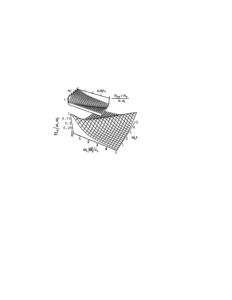
Figure 1: The magnitude of the time-dependent Hamiltonian corresponding to the initial correction as a function of time and distance. The Ohmic ($n=1$) case is shown. The inset demonstrates the onset of the cross-qubit interaction on the same time scale.

.  

First, let us analyze the coherent evolution part in (17), namely, the effect that the imaginary part of $\mathfrak{L}_{\lambda\lambda^{\prime}}(t)$ has on the evolution of the reduced density matrix, since this contribution leads to the induced interaction. If we omitted (18) from (17), (19), and (21), we would obtain the (coherent) evolution operator in the form

$$e^{-i\left(H_{\textrm{int}}+F(t)\right)t}\;.$$ (22)

The interaction $H_{\textrm{int}}$ comes from the first term in (21),

$$H_{\textrm{int}}\!=\!-\frac{2\alpha_{n}^{x}\Gamma(n)c_{s}^{n}\omega_{c}^{n}}{\left(c_{s}^{2}+\omega_{c}^{2}\left|{\mathbf{d}}\right|^{2}\right)^{n/2}}\cos\left[{n\arctan\left({\frac{{\omega_{c}\left|{\mathbf{d}}\right|}}{{c_{s}}}}\right)}\right]\!\sigma_{x}^{1}\sigma_{x}^{2}\,.$$ (23)

This expression gives the constant interaction that is important in large time dynamics. We will obtain this induced exchange interaction latter using different techniques for more general cases, see Sec. 4. The operator $F(t)$ is given by

$$F(t)=2\sigma_{x}^{1}\sigma_{x}^{2}\int\limits_{0}^{\infty}{d\omega\frac{{D(\omega)\left|{g(\omega)}\right|^{2}}}{\omega}\frac{{\sin\omega t}}{{\omega t}}\cos\left(\frac{\omega|\mathbf{d}|}{c_{s}}\right)}\,.$$ (24)

It commutes with $H_{\textrm{int}}$ (and with itself at different times), and therefore $d\left(tF(t)\right)/dt$ can be viewed as the initial time-dependent correction to the interaction. In fact, this term controls the onset of the induced coherent interaction; note that $F(0)=-H_{\textrm{int}}$, but for large times $F(t)\sim\alpha^{x}_{n}\omega_{c}^{n}/(\omega_{c}t)^{n}$.

Let us consider in detail the time dependent correction $H_{F}(t)=d\left(tF(t)\right)/dt$ to the interaction Hamiltonian during the initial evolution,

$$H_{F}(t)=\sigma_{x}^{1}\sigma_{x}^{2}\alpha_{n}\Gamma(n)\Big{[}u(\omega_{c}|\mathbf{d}|/c_{s}-\omega_{c}t)+u(\omega_{c}|\mathbf{d}|/c_{s}+\omega_{c}t)\Big{]}\,,$$ (25)

where $u(\xi)=\cos[n\arctan(\xi)]/(1+\xi^{2})^{n/2}$. The above expression is a superposition of two waves propagating in opposite directions. In the Ohmic case, $n=1$, the shape of the wave is simply $u(\xi)=1/(1+\xi^{2})$.

In Figure 1, we present the amplitude of $H_{F}(t)$, defined via $H_{F}(t)={\cal H}_{F}\sigma_{x}^{1}\sigma_{x}^{2}$, as well as the sum of $H_{\textrm{int}}$ and $H_{F}(t)$, for $n=1$. One can observe that the “onset wave” of considerable amplitude and of shape $u(\xi)$ propagates once between the qubits, “switching on” the interaction. It does not affect the qubits once the interaction has set in. One can also see in Figure 1, as well as from (25), that the interaction between the qubits is delayed by the time $\sim|\mathbf{d}|/c_{s}$, which is required for the mediating (virtual) bosons to carry the response to the other qubit. At the same time, relatively slow decay of the initial correction $F(t)$ may necessitate a discussion regarding the meaning of the “coherent” large-time induced interaction (when the noise effects have also fully set in). We will offer additional comments in the concluding section.

3.2 Initial Dynamics of the Density Matrix Elements and Entanglement

Let us now take the entire solution (17) which includes both the induced interaction discussed above and the noise (18). In the exact solution of the short-time model, the bath is assumed to be thermalized only initially. At large enough times the externally induced equilibration of the bath should be considered. We will account for this later when discussing the perturbative Markovian approach. Here we continue our investigation of the short-time model which assumes that the two qubits coupled with the (noninteracting with each other) bath modes constitute a closed quantum system.

To quantify the interplay of the effects of the induced interaction vs. noise, we evaluate the concurrence,[15, 16] which measures the entanglement of the spin system and is monotonically related to the entanglement of formation.[35, 36] For a mixed state of two qubits, $\rho_{S}$, we first define the spin-flipped state, $\tilde{\rho}_{S}=\sigma^{1}_{y}\sigma^{2}_{y}\,\rho^{*}_{S}\,\sigma^{1}_{y}\sigma^{2}_{y}$, and then the Hermitian operator $R=\sqrt{\sqrt{\rho_{S}}\tilde{\rho}_{S}\sqrt{\rho_{S}}}$, with eigenvalues $\lambda_{i=1,2,3,4}$. The concurrence is then given[16] by

$$C\left({\rho_{S}}\right)=\max\Big{\{}{0,2\mathop{\max}\limits_{i}\lambda_{i}-\sum\limits_{j=1}^{4}{\lambda_{j}}}\Big{\}}\,.$$ (26)

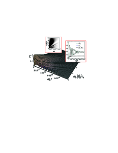
Figure 2: Development of the concurrence as a function of time, calculated with $\alpha_{1}^{z}=0.5\cdot 10^{-7}$ and $k_{\textrm{B}}T/\omega_{c}=0.5\cdot 10^{-2}$, which corresponds to the magnetic field $H_{z}=0.53\,$T and temperatures $T=0.34\,$K. The left inset shows the distribution of the concurrence in the $|\mathbf{d}|$-$t$ plane. The right inset presents the dynamics of the diagonal density matrix elements $P_{++}\equiv\langle++|\rho_{S}(t)|++\rangle$, etc., on the same time scale.

.  

Considering the Si channel geometry for the interaction, introduced above as an illustrative example, we arrive at an approximately adiabatic Hamiltonian ($\alpha_{1}^{z}\gg\alpha_{1}^{x,y}$) with Ohmic-type coupling. The dynamics of the concurrence is presented in Figure 2, and we note that the peak entanglement can reach a sizable fraction of 1. The coupling constant $\alpha_{1}^{z}$ is quite small due to the weakness of the spin-orbit coupling of P-impurity electrons in Si, which results in low magnitude of the induced interaction (and the noise due to the same environment). Nevertheless, one still observes decaying periodic oscillations of entanglement, which indicate that an approximately coherent dynamics can develop, due to the bath-induced interaction, for several dynamical cycles.

To understand the dynamics of the qubit system and its entanglement, let us continue with the analysis of the coherent part in (17). For each spin, we define the two states $\left|\pm\right\rangle=\left[\,\left|\uparrow\right\rangle\pm\left|\downarrow\right\rangle\right]/{\sqrt{2}}$. After the interaction, $H_{\textrm{int}}$, sets in (note the time scales in Figures 1 and 2), it will split the system energies into two degenerate pairs $E_{0}=E_{1}=-{\cal H}_{\textrm{int}}$ and $E_{2}=E_{3}={\cal H}_{\textrm{int}}$. The wave function is then $|\psi(t)\rangle=\exp(-iH_{\textrm{int}}t)|\psi(0)\rangle$. For the initial “++” state, $|\psi(0)\rangle=\left|++\right\rangle$, it develops as $\left|\psi(t)\right\rangle=\left|++\right\rangle\cos{\cal H}_{\textrm{int}}t+\left|--\right\rangle i\sin{\cal H}_{\textrm{int}}t$, where $H_{\textrm{int}}={\cal H}_{\textrm{int}}\sigma^{1}_{m}\sigma^{2}_{m}$. One can easily check that at times $t_{E}=\pi/4{\cal H}_{\textrm{int}},3\pi/4{\cal H}_{\textrm{int}},\ldots$, maximally entangled (Bell) states are obtained, while at times $t_{0}=0,\pi/2{\cal H}_{\textrm{int}},\pi/{\cal H}_{\textrm{int}},\ldots$, the entanglement vanishes; these special times can also be seen in Figure 2.

The coherent dynamics just described is only approximate, because the bath also induces decoherence that enters via (18). The result for the entanglement is that the decaying envelope function is superimposed on the coherent oscillations described above. The magnitudes of the first and subsequent peaks of the concurrence are determined only by this function. As temperature increases, the envelope decays faster resulting in lower values of the concurrence.

Note also that the non-monotonic behavior of the entanglement is possible only provided that the initial state is not trivial with respect to the induced interaction, otherwise only the phase factor is developed. For example, taking the initial state $\left[\,\left|-+\right\rangle+\left|+-\right\rangle\right]/\sqrt{2}$, in our case would only lead to the destruction of entanglement, i.e., to a monotonically decreasing concurrence, similar to results of other studies.[37, 38]

For the model that allows the exact solution, i.e., for $H_{S}=0$, one can notice that there is no relaxation by energy transfer between the system and bath. The exponentials in (17), with (18), suppress only the off-diagonal matrix elements, i.e., those with $\lambda\neq\lambda^{\prime}$. It happens, however, that at large times the $\mathbf{d}$-dependence (the cosine term in $\mathrm{Re}\,\mathfrak{L}_{\lambda\lambda^{\prime}}$) is not important in (18). Therefore, one can show that $\textrm{Re}\,\mathfrak{L}_{\lambda\lambda^{\prime}}(t\rightarrow\infty)$ vanishes for certain combinations of $\lambda\neq\lambda^{\prime}$. Specifically, the limiting $t\to\infty$ density matrix for our initial state ($\left|++\right\rangle$) retains some non-diagonal elements,

$$\rho(t\rightarrow\infty)\rightarrow\frac{1}{8}\left({{\begin{array}[]{*{20}c}3&0&0&{-1}\\ 0&1&1&0\\ 0&1&1&0\\ {-1}&0&0&3\\ \end{array}}}\right)\,.$$ (27)

The basis states here are $\left|++\right\rangle$, $\left|+-\right\rangle$, $\left|-+\right\rangle$, and $\left|--\right\rangle$. The significance of this and similar[39] results is in the fact that in the model with $H_{S}=0$ and non-rethermalizing bath not all the off-diagonal matrix elements need be suppressed by decoherence, even though the concurrence of (27) is zero.

4 INTERPLAY BETWEEN THE INDUCED INTERACTION AND QUANTUM NOISE AT LARGER TIMES

4.1 Master-Equation Approach

In this section we present the expressions for the induced interaction and also for the noise effects due to the bosonic environment, calculated perturbatively to the second order in the spin-boson interaction, and with the assumption that the environment is constantly reset to thermal.[2]

The dynamics of the system can be described by the equation for the density matrix,

$$i\dot{\rho}(t)=[H,\rho(t)]\,.$$ (28)

In order to trace over the bath variables, we carry out the second-order perturbative expansion. This dynamical description is supplemented by the set of Markovian assumptions,[27, 33, 31, 40] one of which invokes resetting the bath to thermal equilibrium, at temperature $T$, after each infinitesimal time step, as well as at time $t=0$, see (16), thereby decoupling the qubit system from the environment.[27, 33] This is a physical assumption appropriate for all but the shortest time scales of the system dynamics.[28, 29, 30] It can also be viewed as a means to phenomenologically account in part for the randomization of the bath modes due to their interactions with each other (anharmonicity) in real systems. This leads to the master equation for the reduced density matrix of the qubits, $\rho_{S}(t)=Tr_{B}\rho(t)$,

$$i\dot{\rho}_{S}(t)=[H_{S},\rho_{S}(t)]-i\!\int\limits_{0}^{\infty}{dt^{\prime}Tr_{B}[H_{SB},[H_{SB}(t^{\prime}-t),\rho_{B}\rho_{S}(t)]]}\,,$$ (29)

where $H_{SB}(\tau)=e^{i(H_{B}+H_{S})\tau}H_{SB}e^{-i(H_{B}+H_{S})\tau}$. Analyzing the structure of the integrand in (29), after lengthy calculations[2] one can obtain the equation with explicitly separated coherent and noise contributions,

$$i\dot{\rho}_{S}(t)=[H_{\textrm{eff}},\rho_{S}(t)]+i{\hat{M}}\rho_{S}(t)\,.$$ (30)

The effective coherent Hamiltonian $H_{\textrm{eff}}$ is

$$H_{\textrm{eff}}\!\!\!=H_{S}+\!\!\!\!\sum\limits_{m=x,y,z}\!\!\!{2\chi_{c}^{m}({\mathbf{d}})\sigma_{m}^{1}\sigma_{m}^{2}}-\chi_{s}^{x}({\mathbf{d}})\left({\sigma_{x}^{1}\sigma_{y}^{2}+\sigma_{x}^{2}\sigma_{y}^{1}}\right)+\chi_{s}^{y}({\mathbf{d}})\left({\sigma_{y}^{1}\sigma_{x}^{2}+\sigma_{y}^{2}\sigma_{x}^{1}}\right)-\left[\eta_{s}^{x}(0)+\eta_{s}^{y}(0)\right]\left({\sigma_{z}^{1}+\sigma_{z}^{2}}\right)\,.$$ (31)

The expressions for the amplitudes $\chi_{c}^{m}(\mathbf{d})$, $\chi_{s}^{m}(\mathbf{d})$, $\eta_{c}^{m}(\mathbf{d})$, and $\eta_{s}^{m}(\mathbf{d})$ will be given bellow. The first three terms following $H_{S}$ constitute the interaction between the two spins. We will argue below that the leading induced exchange interaction is given by the first added term, proportional to $\chi_{c}^{m}(\mathbf{d})$. The last term gives the qubit Lamb shifts.

The otherwise cumbersome expression for the noise terms can be represented concisely by introducing the noise superoperator $\hat{M}$, which involves single-qubit contributions, which are usually dominant, as well as two-qubits terms,

$${\hat{M}}=\sum\limits_{m,i}\Big{[}{\hat{M}}_{m}^{i}(0)+\sum_{j\neq i}{\hat{M}}_{m}^{ij}(\mathbf{d})\Big{]}\,,$$ (32)

where the summations are over the components, $m=x,y,z$, and the qubits, $i,j=1,2$. One can define the superoperators ${\hat{L}}_{a}(O_{1})O_{2}=\{O_{1},O_{2}\}$, ${\hat{L}}(O_{1},O_{2})O_{3}=O_{1}O_{3}O_{2}$, and ${\hat{L}}_{\pm}(O_{1},O_{2})={\hat{L}}(O_{1},O_{2})\pm{\hat{L}}(O_{2},O_{1})$, to write

$${\hat{M}}_{m}^{ij}(\mathbf{d})=\eta_{c}^{m}(\mathbf{d})\left[{2{\hat{L}}(\sigma^{i}_{m},\sigma^{j}_{m})-{\hat{L}}_{a}(\sigma^{i}_{m}\sigma^{j}_{m})}\right]+\eta_{s}^{m}(\mathbf{d})\left[{{\hat{L}}_{+}(\sigma^{i}_{m},\varsigma^{j}_{m})-{\hat{L}}_{a}(\sigma^{i}_{m}\varsigma^{j}_{m})}\right]-i\chi_{s}^{m}(\mathbf{d}){\hat{L}}_{-}(\sigma^{i}_{m},\varsigma^{j}_{m})\,,$$ (33)

where we denote $\varsigma^{j}_{m}=\frac{i}{2}[\sigma_{z}^{j},\sigma_{m}^{j}]$, and

$${\hat{M}}_{m}^{j}(0)=\eta_{c}^{m}(0)\left[{2{\hat{L}}(\sigma_{m}^{j},\sigma_{m}^{j})-{\hat{L}}_{a}(\sigma_{m}^{j}\sigma_{m}^{j})}\right]+\eta_{s}^{m}(0){\hat{L}}_{+}(\sigma_{m}^{j},\varsigma^{j}_{m})-i\chi_{s}^{m}(0)\left[{{\hat{L}}_{-}(\sigma_{m}^{j},\varsigma^{j}_{m})+{\hat{L}}_{a}(\sigma_{m}^{j}\varsigma^{j}_{m})}\right]\,.$$ (34)

The amplitudes in (31), (33), and (34), calculated for the interaction defined in (2)-(3), are

$$\chi_{c}^{m}({\mathbf{d}})=-\sum\limits_{\mathbf{\xi}}{\int\limits_{-\infty}^{\infty}{\frac{{Vd{\mathbf{k}}}}{{\left({2\pi}\right)^{3}}}}}\left|{g_{{\mathbf{k}},\mathbf{\xi}}^{m}}\right|^{2}\frac{{\omega_{{\mathbf{k}},\mathbf{\xi}}\cos\left({{\mathbf{k}}\cdot{\mathbf{d}}}\right)}}{{\omega_{{\mathbf{k}},\mathbf{\xi}}^{2}-\Delta^{2}(1-\delta_{m,z})}}\,,$$ (35)

$$\eta_{c}^{m}({\mathbf{d}})=\frac{\pi}{2}\sum\limits_{\mathbf{\xi}}{\int\limits_{-\infty}^{\infty}{\frac{{Vd{\mathbf{k}}}}{{\left({2\pi}\right)^{3}}}}}\left|{g_{{\mathbf{k}},\mathbf{\xi}}^{m}}\right|^{2}\coth\frac{{\omega_{{\mathbf{k}},\mathbf{\xi}}}}{{2k_{\textrm{B}}T}}\cos\left({{\mathbf{k}}\cdot{\mathbf{d}}}\right)\sum\limits_{q=\pm 1}{\delta\left({\omega_{{\mathbf{k}},\mathbf{\xi}}+(1-\delta_{m,z})q\Delta}\right)}\,,$$ (36)

$$\chi_{s}^{m}({\mathbf{d}})=-\left({1-\delta_{m,z}}\right)\sum\limits_{\mathbf{\xi}}{\int\limits_{-\infty}^{\infty}{\frac{{Vd{\mathbf{k}}}}{{\left({2\pi}\right)^{3}}}}}\left|{g_{{\mathbf{k}},\mathbf{\xi}}^{m}}\right|^{2}\cos\left({{\mathbf{k}}\cdot{\mathbf{d}}}\right)\sum\limits_{q=\pm 1}{\frac{{\pi s}}{2}\delta\left({\omega_{{\mathbf{k}},\mathbf{\xi}}+q\Delta}\right)}\,,$$ (37)

$$\eta_{s}^{m}({\mathbf{d}})=\left({1-\delta_{m,z}}\right)\sum\limits_{\mathbf{\xi}}{\int\limits_{-\infty}^{\infty}{\frac{{Vd{\mathbf{k}}}}{{\left({2\pi}\right)^{3}}}}}\left|{g_{{\mathbf{k}},\mathbf{\xi}}^{m}}\right|^{2}\coth\frac{{\omega_{{\mathbf{k}},\mathbf{\xi}}}}{{2k_{\textrm{B}}T}}\frac{{\Delta\cos\left({{\mathbf{k}}\cdot{\mathbf{d}}}\right)}}{{\omega_{{\mathbf{k}},\mathbf{\xi}}^{2}-\Delta^{2}}}\,.$$ (38)

Here the principal values of integrals are assumed.

Note that $\chi_{c}^{m}({\mathbf{d}})$ appears only in the induced interaction Hamiltonian in (31), whereas $\eta_{c}^{m}({\mathbf{d}})$, $\chi_{s}^{m}({\mathbf{d}})$, and $\eta_{s}^{m}({\mathbf{d}})$ enter both the interaction and noise terms. Therefore, in order to establish that the induced interaction can be significant for some time scales, we have to demonstrate that $\chi_{c}^{m}({\mathbf{d}})$ can have a much larger magnitude than the maximum of the magnitudes of $\eta_{c}^{m}({\mathbf{d}})$, $\chi_{s}^{m}({\mathbf{d}})$, and $\eta_{s}^{m}({\mathbf{d}})$. The third and fourth terms in the expression for the interaction (31) are comparable to the noise and therefore have no significant contribution to the coherent dynamics.

4.2 Qubit Coupling in a 1D Channel

It is instructive to start with the simple 1D example, leaving the derivations for higher dimensions to the next subsection. The 1D geometry can actually be natural for certain ion-trap quantum-computing schemes, in which ions in a chain are subject to Coulomb interaction, developing a variety of phonon-mode lattice vibrations.[24, 25, 26]

In our case we allow the phonons to propagate in a single direction, along $\mathbf{d}$, so that ${\mathbf{k}}\cdot{\mathbf{d}}=k\left|{\mathbf{d}}\right|$. Here, for definiteness, we also assume the linear dispersion, $\omega_{k}=c_{s}k$. Furthermore, we will ignore the polarization index in the coupling constants: $g_{{\mathbf{k}},\mathbf{\xi}}^{m}\to g^{m}(\omega)$.

The induced interaction and noise terms depend on the amplitudes $\chi_{c}^{m}({\mathbf{d}})$, $\eta_{c}^{m}({\mathbf{d}})$, $\chi_{s}^{m}({\mathbf{d}})$, and $\eta_{s}^{m}({\mathbf{d}})$, two of which can be evaluated explicitly for the 1D case, because of the $\delta$-functions in (36), (37). However, to derive an explicit expression for $\chi_{c}^{m}({\mathbf{d}})$ and $\eta_{s}^{m}({\mathbf{d}})$, one needs to specify the $\omega$-dependence in $\left|{g^{m}(\omega)}\right|^{2}$. For the sake of simplicity, in this section we approximate $|g^{m}(\omega)|^{2}$ by a linear function with superimposed exponential cutoff. For a constant 1D density of states $V/2\pi c_{s}$, this is a variant of the Ohmic-dissipation[27] model, i.e., (14) with $n=1$ (the case when $n>1$ is considered in the next subsection).

In most practical applications, we expect that $\Delta\ll\omega_{c}$. With this assumption, we obtain

$$\chi_{c}^{m}({\mathbf{d}})=\frac{{\alpha_{1}^{m}\omega_{c}}}{{1+\left({{{\omega_{c}\left|{\mathbf{d}}\right|}\mathord{\left/{\vphantom{{\omega_{c}\left|{\mathbf{d}}\right|}{c_{s}}}}\right.\kern-1.2pt}{c_{s}}}}\right)^{2}}}\,,$$ (39)

$$\chi_{s}^{m}({\mathbf{d}})=\alpha_{1}^{m}\omega_{c}\frac{\pi}{2}\left({1-\delta_{m,z}}\right)\frac{\Delta}{{\omega_{c}}}\cos\frac{{\Delta\left|{\mathbf{d}}\right|}}{{c_{s}}}\,,$$ (40)

$$\eta_{c}^{m}({\mathbf{d}})=\alpha_{1}^{m}\omega_{c}\frac{\pi}{2}\left({1-\delta_{m,z}}\right)\frac{\Delta}{{\omega_{c}}}\coth\frac{\Delta}{{2k_{\textrm{B}}T}}\cos\frac{{\Delta\left|{\mathbf{d}}\right|}}{{c_{s}}}\,.$$ (41)

The expression for $\eta_{s}({\mathbf{d}})$ could not be obtained in closed form. However, numerical estimates suggest that $\eta_{s}({\mathbf{d}})$ is comparable to $\eta_{c}^{m}({\mathbf{d}})$. At short spin separations $\mathbf{d}$, $\eta_{s}({\mathbf{d}})$ is approximately bounded by $-\alpha_{1}^{m}\Delta\ln\frac{\Delta}{\omega_{c}}\exp(-\frac{{\Delta\left|{\mathbf{d}}\right|}}{{c_{s}}})$, while at lager distances it may be approximated by $\alpha_{1}^{m}\Delta\frac{\pi}{2}\sin\frac{{\Delta\left|{\mathbf{d}}\right|}}{{c_{s}}}\coth\frac{\Delta}{2k_{\textrm{B}}T}$. The level of noise may be estimated by considering the quantity

$${\cal M}=\max_{|\mathbf{d}|}\left|{\eta_{c}^{m}(\mathbf{d}),\chi_{s}^{m}(\mathbf{d}),\eta_{s}^{m}(\mathbf{d})}\right|\,.$$ (42)

The interaction Hamiltonian takes the form

$$H_{\operatorname{int}}=-\frac{2}{{1+\left({{{\omega_{c}\left|{\mathbf{d}}\right|}/{c_{s}}}}\right)^{2}}}\sum\limits_{m=x,y,z}{\alpha_{1}^{m}\omega_{c}\sigma_{m}^{1}\sigma_{m}^{2}}\,.$$ (43)

This induced interaction is temperature independent. It is long-range and decays as a power law for large $\mathbf{d}$. Note that the expression (43) is the same as the induced interaction obtained from the short-time model (23), provided the proper spin-phonon interaction component is considered.

If the noise term were not present, the spin system would be governed by the Hamiltonian $H_{S}+H_{\textrm{int}}$. To be specific, let us analyze the spectrum, for instance, for $\alpha_{1}^{x}=\alpha_{1}^{y}$, $\alpha_{1}^{z}=0$. The two-qubit states would consist of the singlet $(\left|{\uparrow\downarrow}\right\rangle-\left|{\downarrow\uparrow}\right\rangle)/\sqrt{2}$ and the split triplet $\left|{\uparrow\uparrow}\right\rangle$, $(\left|{\uparrow\downarrow}\right\rangle+\left|{\downarrow\uparrow}\right\rangle)/\sqrt{2}$, and $\left|{\downarrow\downarrow}\right\rangle$, with energies $E_{2}=-4\chi_{c}^{x}$, $E_{0}=-\Delta$, $E_{1}=4\chi_{c}^{x}$, $E_{3}=\Delta$, respectively. The energy gap $|E_{1}-E_{2}|$ between the two entangled states is defined by $4\chi_{c}^{x}$ ($=4\chi_{c}^{y}$). In the presence of noise, the oscillatory, approximately coherent evolution of the spins can be observed over several oscillation cycles provided that $2\alpha_{1}^{m}\omega_{c}/[1+(\omega_{c}|\mathbf{d}|/c_{s})^{2}]>{\cal M}$. The energy levels will acquire effective width due to quantum noise, of order $\eta_{c}^{m}(\mathbf{d})$.

4.3 Boson-Mediated Induced Qubit-Qubit Interaction in General Dimensions

Let us generalize the results of the previous subsections, where we considered the 1D case with Ohmic dissipation within the Markovian approach. In the general case, let us consider the Markovian model and, again, assume that $\Delta/\omega_{c}$ is small. We will also assume that the absolute square of the $m$th component of the spin-boson coupling, when multiplied by the density of states, can be modeled by $\alpha_{n_{m}}^{m}{}\omega^{n_{m}}\exp(-\omega/\omega_{c})$; see (14). The integration in (35) can then be carried out in closed form for any $n_{m}=1,2,\ldots\,\,$. The induced interaction (43) is thus generalized to

$$H_{\textrm{int}}=-\!\!\!\sum\limits_{m=x,y,z}{\alpha_{n_{m}}^{m}\omega_{c}^{n_{m}}\sigma_{m}^{1}\sigma_{m}^{2}}\frac{{2\Gamma(n_{m})\textrm{Re}\left({1+i\omega_{c}\left|{\mathbf{d}}\right|/c_{s}}\right)^{n_{m}}}}{{\left[{1+\left({\omega_{c}\left|{\mathbf{d}}\right|/c_{s}}\right)^{2}}\right]^{n_{m}}}}\,.$$ (44)

With the appropriate choice of parameters, the result for the induced interaction, but not for the noise, coincides with the expression for $H_{\textrm{int}}$ obtained within the short-time model. The effective interaction has the large-distance asymptotic behavior $\left|{\mathbf{d}}\right|^{-n_{m}}$, for even $n_{m}$, and $\left|{\mathbf{d}}\right|^{-n_{m}-1}$, for odd $n_{m}$.

In higher dimensions the structure of $g_{{\mathbf{k}},\mathbf{\xi}}^{m}$ in the k-space becomes important. Provided $\omega_{{\mathbf{k}},\mathbf{\xi}}$ is nearly isotropic, the integrals in (35)-(38) will include (in 3D) a factor $\int_{0}^{2\pi}{d\varphi}\int_{0}^{\pi}{d\theta\sin\theta}\left|{g_{k\theta\varphi,\mathbf{\xi}}^{m}}\right|^{2}\cos\left({k\left|{\mathbf{d}}\right|\cos\theta}\right)$, which can be written as $[f^{m}_{1}(\omega,k|\mathbf{d}|)-f^{m}_{2}(\omega,k|\mathbf{d}|)\partial/\partial|\mathbf{d}|]\cos(k|\mathbf{d}|)$, see Eqs. (B1)-(B4) of Ref. 2 for details. When the dependence of $f^{m}_{1},f^{m}_{2}$ on $k|\mathbf{d}|$ is negligible, the interaction is simply $H_{\textrm{int}}\rightarrow H_{\textrm{int}}|_{\{n_{m}\}\rightarrow a}-(\partial/\partial|\mathbf{d}|)H_{\textrm{int}}|_{\{n_{m}\}\rightarrow b}$, where $a$ and $b$ are sets of three integers representing the $\omega$-dependence of $f_{1}^{m}(\omega,k|\mathbf{d}|)$ and $f_{2}^{m}(\omega,k|\mathbf{d}|)$. Otherwise, a more complicated dependence on $|\mathbf{d}|$ is expected. The noise superoperator can be treated similarly.

4.4 Induced Interaction vs. Noise in the Semiconductor Impurity Qubit Model

Let us now proceed to an example of the semiconductor qubit model in the bulk material, which gives usual 3D geometry for phonon propagation. We consider spins of P-impurity donor electrons as qubits. Dilute P-impurities are embedded in the matrix of a Si or Ge crystal kept at a sufficiently low temperature such that the outer electrons remain bound. The two impurities placed next to each other at distances of about 10-30 nm would constitute a two qubit register. The spins would then be interacting indirectly via the spin-orbit coupling and lattice deformation (phonons) as well as directly via the dipole-dipole electromagnetic coupling. In this section we will estimate and compare both. We will also present the dynamics due to the coherent vs. noise induced features and their interplay.

Let us consider for simplicity only the LA phonon branch, ${\mathbf{\xi}}\to{\mathbf{k}}/\left|{\mathbf{k}}\right|$, and assume an isotropic dispersion $\omega_{\mathbf{k},\mathbf{\xi}}=c_{s}\left|\mathbf{k}\right|$. The expression for the coupling constants is then

$$g_{{\mathbf{k}},{\mathbf{\xi}}}^{m}=D_{m}\frac{{k_{z}k_{m}}}{{\left({1+a_{\textrm{B}}^{2}k^{2}}\right)^{2}}}\sqrt{\frac{\hbar}{{2\rho Vc_{s}k^{3}}}}\,.$$ (45)

One can show[2] that the cross terms, with $m\neq n$, of the correlation functions $Tr_{B}\left[X_{m}^{j}X_{n}^{i}(t)\rho_{B}\right]$, depend on the combination $g_{\mathbf{k},\mathbf{\xi}}^{m}(g_{\mathbf{k},\mathbf{\xi}}^{n})^{*}$, which is always an odd function of one of the projections of the wave vector. Thus, all the non-diagonal terms vanish.

Integrating (35) and (36) with (45), one can demonstrate[2] that decoherence is dominated by the individual noise terms for each spin, with the typical amplitude

$$\eta_{c}^{x,y}(0)=C_{\textrm{B}}\frac{{2\pi^{2}}}{{15}}\frac{b^{3}}{\left({1+b^{2}}\right)^{4}}\coth\frac{\Delta}{2k_{\textrm{B}}T}\,,$$ (46)

where $b=\Delta a_{\rm B}/c_{s}$ and $C_{\textrm{B}}={\rm B}^{2}\mu_{\textrm{B}}^{2}H_{z}^{2}/\left({16\pi^{3}\rho\hbar a_{\rm B}^{3}c_{s}^{2}}\right)$. The interaction amplitude $\chi_{c}^{m}({\mathbf{d}})$ and, therefore, the induced spin-spin interaction, have inverse-square power-law asymptotic form for the $x$ and $y$ spin components, with a superimposed oscillation, and inverse-fifth-power-law decay for the $z$ spin components,

$$H_{\textrm{int}} = \sum\nolimits_{m}{2\chi_{c}^{m}({\mathbf{d}})\sigma_{m}^{1}\sigma_{m}^{2}}$$

$$\xrightarrow{{r\gg 1}} -4\pi^{2}C_{\textrm{B}}\frac{{2b}}{{\left({1+b^{2}}\right)^{4}}}\frac{{\sin br}}{{r^{2}}}\left({\sigma_{x}^{1}\sigma_{x}^{2}+\sigma_{y}^{1}\sigma_{y}^{2}}\right)+384\pi^{2}C_{\textrm{A}}\frac{2}{{r^{5}}}\sigma_{z}^{1}\sigma_{z}^{2}$$

$$\xrightarrow{{r\ll 1}} \left[-4\pi^{2}C_{\mathrm{B}}\frac{1+9b^{2}-9b^{4}+b^{6}}{120(1+b^{2})^{4}}+{\cal O}(r^{2})\right]\left({\sigma_{x}^{1}\sigma_{x}^{2}+\sigma_{y}^{1}\sigma_{y}^{2}}\right)+\left[-C_{\mathrm{A}}\frac{\pi^{2}}{10}+{\cal O}(r^{2})\right]\sigma_{z}^{1}\sigma_{z}^{2}\,.$$

Here $r=|\mathbf{d}|/a_{\textrm{B}}$ and $C_{\textrm{A}}=\textrm{A}^{2}C_{\textrm{B}}/\textrm{B}^{2}$. At small distances the interaction is regular and the amplitudes converge to constant values, see Figure 3. The complete expressions for $\chi_{c}^{m}(\mathbf{d})$ and $\eta_{c}^{m}(\mathbf{d})$ are also available.[2]

In Figure 3, we plot the amplitudes of the induced spin-spin interaction, which has the asymptotic behavior (4.4), and noise for different values of the spin-spin separation and $b$, for electron impurity spins in 3D Si-Ge type structures. The value of $b$ can be controlled via the applied magnetic field, $b=\mu_{\textrm{B}}H_{z}g^{*}a_{\textrm{B}}/c_{s}$. The temperature dependence of the noise is insignificant provided $2k_{\textrm{B}}T/\Delta\ll 1$.

As mentioned earlier, the obtained interaction (4.4) is always accompanied by noise coming from the same source, as well as by the direct interactions of the spins. When the electron wave functions overlap is negligible, the dominant direct interaction will be the electromagnetic dipole-dipole one,

$$H_{\textrm{EM}}(\mathbf{d})=\frac{\mu_{0}\mu_{\textrm{B}}^{2}}{4\pi}\frac{\sigma_{x}^{1}\sigma_{x}^{2}+\sigma_{y}^{1}\sigma_{y}^{2}-2\sigma_{z}^{1}\sigma_{z}^{2}}{|\mathbf{d}|^{3}}\,.$$ (48)

The comparison of the two interactions and noise is shown in Figure 4. We plot the magnitude of the effective induced interaction (4.4), the electromagnetic interaction (48), measured by ${\cal H}_{\textrm{EM}}\equiv{\mu_{0}\mu_{\textrm{B}}^{2}}/{4\pi|\mathbf{d}|^{3}}$, and a measure of the level of noise, for P-donor electron spins in Ge. In the plot the coupling constants for P-donors in Ge were taken as $C_{\textrm{B}}=1.3\times{}10^{7}\,$s^-1 and $C_{\textrm{A}}\approx 0$, see Sec. 2. It transpires that the induced interaction can be considerable as compared to the electromagnetic spin-spin coupling. However the overall coherence-to-noise ratio is quite poor for Ge. In Si, the level of noise is lower as compared to the induced interaction. It is dominated primarily by the adiabatic ($\sigma_{z}^{1,2}$) term. However, the overall amplitude of the induced terms compares less favorably with the electromagnetic coupling.

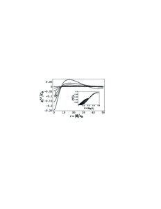
Figure 3: The magnitude of the induced spin-spin interaction for a 3D Si-Ge type structure: the dominant interaction amplitude, which is the same for the $x$ and $y$ spin components, is shown. The arrow indicates increasing $b$ values for the curves shown, with $b=\Delta a_{\rm B}/c_{s}=0.03$, $0.09$, $0.15$, $0.21$, $0.27$, $0.33$. The inset estimates the level of the noise (for $2k_{\textrm{B}}Ta_{\rm B}/c_{s}=0.01$): the bottom curve is $\eta_{c}^{m}(0)$, with $m=x,y$. For $b\leq 0.4$, the amplitude $\eta_{s}^{m}(\mathbf{d})$ can be comparable, and its values, calculated numerically for $0\leq r\leq 50$, are shown as long as they exceed $\eta_{c}^{m}(0)$, with the top curve corresponding to the maximum value, at $r=0$.

.  

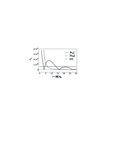
Figure 4: The magnitudes, measured in units of s^-1, of the induced spin-spin interaction, the dipole-dipole coupling strength, and the level of noise for P-impurity electron spins in Ge. Here $H_{z}=3\times 10^{4}\,$G, and low temperature, $2k_{\textrm{B}}T/\Delta\ll 1$, was assumed.

.  

Let us estimate the development of entanglement for the P-in-Si case, considering only the bath-induced effects. Taking $\left|++\right\rangle$ as the initial state, one expects entanglement to develop due to the ${\cal H}_{\textrm{int}}\sigma_{z}^{1}\sigma_{z}^{2}$ interaction term. The corresponding coupling constant is $C_{\textrm{B}}=7800\,$s^-1. At distances of about $12a_{\textrm{B}}$ this part of the interaction can be already well approximated by ${\cal H}_{\textrm{int}}\sim 384\pi^{2}C_{\textrm{A}}\frac{2a_{\textrm{B}}^{5}}{{|\mathbf{d}|^{5}}}\sim 100\,$s^-1. The $x$ and $y$ components of the interaction are smaller by a factor $10^{-3}$ and will not be considered. The pure state would then be developing as $\left|\psi(t)\right\rangle=\left|++\right\rangle\cos{\cal H}_{\textrm{int}}t+\left|--\right\rangle i\sin{\cal H}_{\textrm{int}}t$. At times $t_{E}=\pi/4{\cal H}_{\textrm{int}},3\pi/4{\cal H}_{\textrm{int}},\ldots$, the maximally entangled (Bell) states are obtained, with the first occurring at $\simeq 0.8\cdot 10^{-2}\,$s, and then at intervals of $\simeq 1.6\cdot 10^{-2}\,$s. The actual entanglement is lowered by (i) the short-time (adiabatic) decoherence term, (ii) the large-time relaxation amplitudes (rates). The latter are due to the $x,y$ components of the qubit-bath coupling and are of order $\sim 1\,$s^-1. As a result the first peak of the concurrence is lowered by a factor of $\sim\exp(-0.8\cdot 10^{-2})$, and the subsequent peaks decrease by $\sim\exp(-1.6\cdot 10^{-2})$ per each cycle.

A

5 DISCUSSION OF OPEN PROBLEMS

We have studied the induced indirect exchange interaction due to a bosonic bath which also introduces quantum noise. At certain time scales the induced two-qubit interaction is sufficiently strong to produce significant coherent effects. This interaction can be a factor to be considered in designs of solid state (as well as ion-trap based) qubit registers. Even more importantly, the fact that noise-inducing environment can also yield coherent features in the dynamics of open quantum systems poses several interesting fundamental challenges.

The usual approach to thermalization[33, 31, 40, 41, 42] has been to assume that, for large enough times, the time evolution of the system plus bath is not just covered by the combined Hamiltonian, but is supplemented by the instantaneous loss-of-memory (Markovian) approximation, which introduces irreversibility and imposes the bath temperature on the reduced system dynamics in the infinite-time limit, which is then approached as the density matrix elements assume their thermal values, according to

$$\rho_{S}(t)\to{{e^{-H_{S}/kT}}\Big{/}{{{Tr}}\left({e^{-H_{S}/kT}}\right)}}\,,$$ (49)

with exponential relaxation (diagonal) and decoherence (off-diagonal) rates defining the time scales $T_{1,2}$. However, it turns out that the traditional phenomenological no-memory approximations, yielding thermalization, the Fermi golden rule for the transition rates, etc., assume in a way too strong a memory loss: they erase the possible bath contributions to the coherent part of the dynamics at shorter times, such as the Lamb shift for a single system as well as the induced RKKY interactions for a bi-partite system. Indeed, while relaxation leading to (49) is driven by the “on-shell” exchanges with the bath, it is the memory of (correlation, entanglement with) the bath modes that drives, via virtual exchanges, the induced interaction. Actually, the “on-shell” condition, imposed by the so-called secular approximation,[7] also underestimates additional decoherence at short times — the “pure” or “adiabatic” contribution to the off-diagonal dephasing — that has thus been estimated by using other approaches.[43, 28, 44, 29, 45]

Perhaps the simplest way to recognize the ambiguity is to ask if the Hamiltonian in (49) should have included the bath-induced interaction terms (not shown)? Should the final Boltzmann distribution correspond to the energy levels/basis states of the original “bare” system or the one with the RKKY-interaction/Lamb shifts, and more generally, a bath-renormalized, “dressed” system?

There is presently no consistent treatment that will address in a satisfactory way all the expected physics of the bath-mode effects on the dynamics. The issue is partly technical, because we are after a tractable, rather than just a “foundational” answer. It is well accepted that the emergence of irreversibility cannot be fully treated within tractable and calculationally convenient approaches derived directly from the microscopic dynamics: phenomenology has to be appealed to. However, even allowing for phenomenological solutions, most of the known tractable Markovian-approximation-involving schemes that allow for the emergence of the indirect exchange interaction, treat thermalization in a cavalier way, yielding typically the noise term corresponding to $T$-dependent relaxation, but in the strict $t\to\infty$ limit resulting in the completely random ($T=\infty$) density matrix (proportional to the unit operator). This then avoids the issue of which $H_{S}$ should enter in (49). And, as mentioned, the established schemes that yield a more realistic, thermalized density matrix at $t=\infty$, lose some intermediate- and short-time dynamical effects.

Thus, we have discussed the challenges in formulating unified treatments that will cover all the (or just most of the interesting) dynamical effects, over several time scales, from short to intermediate times (for induced interaction effects and pure decoherence) to large times (for the onset of thermalization), while providing a tractable calculational (usually perturbative, many-body) scheme. This discussion also alludes to several other interesting conceptual challenges in the theory of open quantum systems.

Let us presently comment on the issue of the bath-mode interactions with each other, as well as with impurities, the latter particularly important and experimentally relevant[46, 47] for conduction electrons as carriers of the indirect-exchange interaction. Indeed, the traditional treatment of open quantum systems has assumed noninteracting bath modes. When the bath mode interactions had to be accounted for, the added effects were treated either perturbatively,[48] or, for strong interaction, such as Luttinger-liquid electrons in a 1D channel, the collective excitations were taken[49] as the new “bath modes.” Generally, however, especially in Markovian schemes, one has to seek approaches that do not involve certain double-counting. Indeed, the assumption that the bath modes are at a fixed temperature, could be possibly considered as partially accounting for the effects of the mode-mode and mode-impurity interactions, because these interactions can contribute to thermalization of the bath, on par with other influences external to the bath. This may be particularly relevant for phonons that always have strong anharmonicity for any real material. In a way this problem fits with the previous one: we are dealing with effects that can be, on one hand, modeled by added terms in the total Hamiltonian but on the other hand, may be also mixed in the process of thermalization that is modeled by actually departing from the Hamiltonian description and replacing it with Liouville equations that include noise effects. While all this sounds somewhat “foundational,” recent experimental advances, interestingly, bring these challenges to the level of application that requires tractable, albeit perhaps phenomenological solutions that can be directly confronted with experimental data.

There are other interesting topics to be considered, for instance, the question of whether additional sources of quantum noise are possible? For instance, it has been recently established[50] that potential difference between two leads (reservoirs, or baths, of electrons) can be a source of quantum noise with the potential difference playing the role of the temperature parameter.

As an example of a more practical issue to be investigated, let us mention the possible effect of the sample geometry on phonon and conduction electron induced relaxation and interactions. The one-dimensional aspect of the electron gas in a channel has already been explored.[49] Indeed, electrons are easy to confine by gate potentials. The situation for phonons, however, is less clear: can geometrical effects modify, and particularly reduce, their quantum-noise generation capacity, or change the induced interactions? Our preliminary studies reviewed in this article, seem to indicate strong overall geometry dependence of the exchange interactions. However, the situation is not entirely clear, especially for the strength of the noise effects, and requires a full scale exploration because recent experiments with double dot nanostructures in Si membranes[51] suggest that true nanosize confinement (due to the sample dimensions) of otherwise long-wavelength modes (in the transverse sample dimensions) is now possible and will have dramatic effect on the phonon spectrum and, as a result, on those physical phenomena that depend on the phonon interactions with electron spins.

- [1] D. Solenov, D. Tolkunov, and V. Privman, Phys. Lett. A 359, 81 (2006).
- [2] D. Solenov, D. Tolkunov, and V. Privman, Phys. Rev. B 75, 035134 (2007).
- [3] M. Xiao, I. Martin, E. Yablonovitch, and H. W. Jiang, Nature 430, 435 (2004).
- [4] M. R. Sakr, H. W. Jiang, E. Yablonovitch, and E. T. Croke, Appl. Phys. Lett. 87, 223104 (2005).
- [5] N. J. Craig, J. M. Taylor, E. A. Lester, C. M. Marcus, M. P. Hanson, and A. C. Gossard, Science 304, 565 (2004).
- [6] J. M. Elzerman, R. Hanson, L. H. Willems van Beveren, B. Witkamp, L. M. K. Vandersypen, and L. P. Kouwenhoven, Nature 430, 431 (2004).
- [7] F. H. L. Koppens, C. Buizert, K. J. Tielrooij, I. T. Vink, K. C. Nowack, T. Meunier, L. P. Kouwenhoven, and L. M. K. Vandersypen, Nature 442, 766 (2006).
- [8] J. R. Petta, A. C. Johnson, J. M. Taylor, E. A. Laird, A. Yacoby, M. D. Lukin, C. M. Marcus, M. P. Hanson, and A. C. Gossard, Science 309, 2180 (2005).
- [9] I. Martin, D. Mozyrsky, and H. W. Jiang, Phys. Rev. Lett. 90, 018301 (2003).
- [10] E. Prati, M. Fanciulli, A. Kovalev, J. D. Caldwell, C. R. Bowers, F. Capotondi, G. Biasiol, and L. Sorba, IEEE Trans. Nanotechnol. 4, 100 (2005).
- [11] Y. Nakamura, Y. A. Pashkin, and J. S. Tsai, Nature (London) 398, 786 (1999).
- [12] D. Vion, A. Aassime, A. Cottet, P. Joyez, H. Pothier, C. Urbina, D. Esteve, and M. H. Devoret, Science 296, 886 (2002).
- [13] I. Chiorescu, Y. Nakamura, C. J. P. Harmans, and J. E. Mooij, Science 299, 1869 (2003).
- [14] T. Yamamoto, Y. A. Pashkin, O. Astafiev, Y. Nakamura, and J. S. Tsai, Nature (London) 425, 941 (2003).
- [15] S. Hill and W. K. Wootters, Phys. Rev. Lett. 78, 5022 (1997).
- [16] W. K. Wootters, Phys. Rev. Lett. 80, 2245 (1998).
- [17] G. D. Mahan, Many-Particle Physics (Kluwer Academic, New York, 2000).
- [18] H. Hasegawa, Phys. Rev. 118, 1523 (1960).
- [19] L. M. Roth, Phys. Rev. 118, 1534 (1960).
- [20] R. Winkler, Spin-Orbit Coupling Effects in Two-Dimentional Electron and Hole Systems (Springer, New York, 2003).
- [21] T. Pellizzari, S. A. Gardiner, J. I. Cirac, and P. Zoller, Phys. Rev. Lett. 75, 3788 (1995).
- [22] D. Mozyrsky, Sh. Kogan, V. N. Gorshkov, and G. P. Berman, Phys. Rev. B 65, 245213 (2002).
- [23] M. Asheghi, Y. K. Leung, S. S. Wong, and K. E. Goodson, Appl. Phys. Lett. 71, 1798 (1997).
- [24] D. Leibfried, R. Blatt, C. Monroe, and D. Wineland, Rev. Mod. Phys. 75, 281 (2003).
- [25] C. Marquet, F. Schmidt-Kaler, and D. F. V. James, Appl. Phys. B 76, 199 (2003).
- [26] D. Porras and J. I. Cirac, Phys. Rev. Lett. 92, 207901 (2004).
- [27] A. J. Leggett, S. Chakravarty, A. T. Dorsey, M. P. A. Fisher, A. Garg, and W. Zwerger, Rev. Mod. Phys. 59, 1 (1987).
- [28] V. Privman, Modern Phys. Lett. B 16, 459 (2002).
- [29] D. Tolkunov and V. Privman, Phys. Rev. A 69, 062309 (2004).
- [30] D. Solenov and V. Privman, Int. J. Modern Phys. B 20, 1476 (2006).
- [31] W. H. Louisell, Quantum Statistical Properties of Radiation (Wiley, New York, 1973).
- [32] G. M. Palma, K.-A. Suominen, and A. K. Ekert, Proc. R. Soc. London Ser. A 452, 576 (1996).
- [33] N. G. van Kampen, Stochastic Processes in Physics and Chemistry (North-Holland, Amsterdam, 2001).
- [34] R. Doll, M. Wubs, P. Hänggi, and S. Kohler, e-print: cond-mat/0703075 (at www.arxiv.org).
- [35] C. H. Bennett, D. P. DiVincenzo, J. A. Smolin, and W. K. Wootters, Phys. Rev. A 54, 3824 (1996).
- [36] V. Vedral, M. B. Plenio, M. A. Rippin, and P. L. Knight, Phys. Rev. Lett. 78, 2275 (1997).
- [37] T. Yu and J. H. Eberly, Phys. Rev. B 68, 165322 (2003).
- [38] T. Yu and J. H. Eberly, Phys. Rev. Lett. 93, 140404 (2004).
- [39] D. Braun, Phys. Rev. Lett. 89, 277901 (2002).
- [40] K. Blum, Density Matrix Theory and Applications (Plenum Press, New York, 1996).
- [41] A. Abragam, Principles of Nuclear Magnetism (Clarendon Press, 1983).
- [42] C. P. Slichter, Principles of Magnetic Resonance (Springer, 1991).
- [43] A. Fedorov, L. Fedichkin, and V. Privman, J. Comp. Theor. Nanosci. 1, 132 (2004).
- [44] V. Privman, J. Stat. Phys. 110, 957 (2003).
- [45] E. Paladino, M. Sassetti, G. Falci, and U. Weiss, Chem. Phys. 322, 98 (2006).
- [46] M. R. Sakr, E. Yablonovitch, E. T. Croke, and H. W. Jiang, e-print: cond-mat/0504046 (at www.arxiv.org).
- [47] H. W. Jiang, private communication.
- [48] D. Mozyrsky, V. Privman, and I. D. Vagner, Phys. Rev. B 63, 085313 (2001).
- [49] D. Mozyrsky, A. Dementsov, and V. Privman, Phys. Rev. B 72, 233103 (2005).
- [50] D. Mozyrsky and I. Martin, Phys. Rev. Lett. 89, 018301 (2002).
- [51] P. Zhang, E. Tevaarwerk, B.-N. Park, D. E. Savage, G. K. Celler, I. Knezevic, P. G. Evans, M. A. Eriksson, and M. G. Lagally, Nature 439, 703 (2006).