Condensates of Strongly-interacting Atoms
and Dynamically Generated Dimers

Abstract

In a system of atoms with large positive scattering length, weakly-bound diatomic molecules (dimers) are generated dynamically by the strong interactions between the atoms. If the atoms are modeled by a quantum field theory with an atom field only, condensates of dimers cannot be described by the mean-field approximation because there is no field associated with the dimers. We develop a method for describing dimer condensates in such a model based on the one-particle-irreducible (1PI) effective action. We construct an equivalent 1PI effective action that depends not only on the classical atom field but also on a classical dimer field. The method is illustrated by applying it to the many-body behavior of bosonic atoms with large scattering length at zero temperature using an approximation in which the 2-atom amplitude is treated exactly but irreducible $N$-atom amplitudes for $N\geq 3$ are neglected. The two 1PI effective actions give identical results for the atom superfluid phase, but the one with a classical dimer field is much more convenient for describing the dimer superfluid phase. The results are also compared with previous work on the Bose gas near a Feshbach resonance.

I Introduction

The development of the technology for cooling atoms to ultralow temperatures led to the discovery of Bose-Einstein condensation in dilute atomic gases Anderson1995a ; Davis1995b ; Bradley1995a . It opened up the possibility for experimental study of Bose gases. By controlling the scattering length of the atoms using Feshbach resonances, it is possible to study strongly-interacting Bose gases Inouye98 ; Courteille98 ; Roberts98 . Among the interesting phenomena that have been observed is atom-molecule coherence Donley-nature2002-417 ; Cla02 ; Rb-85-data , which is characterized by oscillations whose frequency coincides with the binding energy of a diatomic molecule.

There have been several studies of a Bose gas of atoms near a Feshbach resonance. Radzihovsky, Park, and Weichman RPW and Romans, Duine, Sachdev, and Stoof RDSS predicted that in addition to the normal phase and an atomic superfluid phase, there is a molecular superfluid phase. In the atomic superfluid phase, there is a Bose-Einstein condensate of atoms and there may also be a Bose-Einstein condensate of diatomic molecules (dimer condensate). In the molecular superfluid phase, there is a dimer condensate but no atom condensate. Lee and Lee used the renormalization group to study the nature of the phase transition between the atomic superfluid and the molecular superfluid LL . Basu and Mueller studied various instabilities of the superfluid phases BM . The studies of Refs. RPW and RDSS indicate that at zero temperature, there is a quantum phase transition between the atomic superfluid and the molecular superfluid. The relevant interaction parameter is the detuning energy of the molecule or, equivalently, the scattering length $a$ of the atoms. The quantum phase transition occurs at a positive critical value $a_{c}$ of the scattering length that depends on the number density.

A Feshbach resonance allows the scattering length $a$ to be tuned arbitrarily large. When the scattering length $a$ is large compared to the range (and all other length scales set by the interactions), identical bosons have universal few-body properties that are determined by $a$ and governed by a discrete scaling symmetry Braaten:2004rn . Efimov showed in 1970 Efimov:1970 that in the unitary limit $a=\pm\infty$, there are infinitely many arbitrarily shallow 3-body bound states (called Efimov trimers). Their binding energies have a geometric spectrum:

$$E_{T}^{(n)}={22.7}^{-2(n-n_{*})}\hbar^{2}\kappa_{*}^{2}/m\ ,$$ (1)

where $m$ is the mass of the bosons and $\kappa_{*}$ is the binding wavenumber of the Efimov trimer labelled by $n_{*}$. We will refer to $\kappa_{*}$ as the Efimov parameter. The spectrum in Eq. (1) is consistent with a discrete scaling symmetry with discrete scaling factor $e^{\pi/s_{0}}\approx 22.7$, where $s_{0}\approx 1.00624$ is a transcendental number. Efimov showed that the discrete scaling symmetry is also relevant when $a$ is large but not infinite Efimov:1971 ; Efimov:1979 . For example, few-body observables involving only particles with zero momentum must have the form $a^{p}\ f(s_{0}\log(a\kappa_{*}))$, where $p$ is the power required by dimensional analysis and $f(\theta)$ is a dimensionless function with period $2\pi$. We will refer to such log-periodic behavior as Efimov physics.

In the previous analyses of the strongly-interacting Bose gas in Refs. RPW ; RDSS ; LL ; BM , Efimov physics has been completely ignored. An obvious qualitative consequence of Efimov physics is the possible existence of a trimer superfluid phase in which there is a Bose-Einstein condensate of Efimov trimers (trimer condensate), but no atom condensate or dimer condensate. The methods used in Refs. RPW ; RDSS ; LL ; BM would be incapable of describing a trimer superfluid phase. In these analyses, the model used as a starting point was a quantum field theory with quantum fields $\hat{\psi}_{A}({\bf r},t)$ and $\hat{\psi}_{M}({\bf r},t)$ that annihilate an atom and a molecule, respectively. Most of the quantitative analyses in Refs. RPW ; RDSS were carried out using the mean-field approximation. The order parameters associated with the atomic superfluid and molecular superfluid phases were the mean fields $\langle\hat{\psi}_{A}\rangle$ and $\langle\hat{\psi}_{M}\rangle$, respectively. In the atomic superfluid phase, $\langle\hat{\psi}_{A}\rangle\neq 0$ and $\langle\hat{\psi}_{M}\rangle\neq 0$, while in the molecular superfluid phase, $\langle\hat{\psi}_{M}\rangle\neq 0$ and $\langle\hat{\psi}_{A}\rangle=0$. If the scattering length in this model is tuned to be sufficiently large, Efimov trimers will be generated dynamically by the strong interactions between the atoms. However the mean-field approximation cannot reveal the existence of a trimer superfluid phase, because there is no quantum field whose expectation value can indicate the presence of a condensate of Efimov trimers.

There is an analogous problem with the dimer superfluid phase in a quantum field theory with only an atom field $\hat{\psi}_{A}({\bf r},t)$. If the scattering length $a$ is positive and sufficiently large, the dimer is generated dynamically by the strong interactions between the atoms. The mean field $\langle\hat{\psi}_{A}\rangle$ provides an order parameter for the atom superfluid phase. However the mean-field approximation cannot reveal the existence of a dimer superfluid phase, because there is no quantum field whose expectation value can indicate the presence of a condensate of dimers.

In this paper, we show how a dimer superfluid phase can be studied in a quantum field theory in which the only quantum field is the atom field $\hat{\psi}_{A}({\bf r},t)$. Our basic tool is the one-particle-irreducible (1PI) effective action $\Gamma[A]$, which is a functional of a classical atom field $A({\bf r},t)$. This effective action encodes complete information about the quantum system. The variational equations for the 1PI effective action provide a straightforward description of states containing an atom condensate or a mixture of an atom condensate and a dimer condensate. They also contain complete information about states containing a dimer condensate but no atom condensate, but this information is encoded in a more subtle form. We show how one can construct an equivalent effective action $\Gamma[A,D]$ that is also a functional of a classical dimer field $D({\bf r},t)$. This effective action provides a straightforward description of states containing a dimer condensate but no atom condensate.

In section II, we introduce the 1PI effective action for a quantum field theory. We determine the 1-body and 2-body terms $\Gamma_{1+2}[A]$ in the 1PI effective action for the zero-range model. In this model, the only interaction is a contact interaction that gives the large scattering length $a$. Any other model with a large scattering length should reduce to the zero-range model when $|a|$ is sufficiently large. In the case $a>0$, we construct the equivalent terms $\Gamma_{1+2}[A,D]$ in an effective action with a classical dimer field. In section III, we consider the approximation defined by the truncated 1PI effective actions $\Gamma_{1+2}[A]$ and $\Gamma_{1+2}[A,D]$. This truncated 1PI approximation corresponds to treating 2-atom quantum effects exactly, but ignoring irreducible 3-atom and higher $N$-atom effects. To demonstrate the limitations of this approximation, we use it to calculate the atom-dimer scattering cross-section. The results are compared with those from exact solutions of the 3-body problem, which depend on the Efimov parameter $\kappa_{*}$. In section IV and V, we demonstrate the equivalence of the truncated 1PI effective actions by using them to study the strongly-interacting Bose gas with total atom number density $n$ at zero temperature. In section IV, we study the static homogeneous states. There is an atom superfluid phase and a dimer superfluid phase separated by quantum phase transitions at $a=0$ and $a=(32\pi n)^{-1/3}$. In section V, we study the quasiparticles associated with fluctuations around the static homogeneous states. The two truncated 1PI effective actions give identical results for the atom superfluid phase, but $\Gamma_{1+2}[A,D]$ is much more convenient for describing the dimer superfluid phase. In section VI, we summarize our results and discuss their implications for the Bose gas near a Feshbach resonance.

II 1PI Effective Action

In this section, we introduce the 1PI effective action for a quantum field theory of bosons. If there is a single atom quantum field, the 1PI effective action $\Gamma[A]$ is a functional of a classical atom field $A$ that encodes complete information on quantum effects. The one-body and two-body terms $\Gamma_{1+2}[A]$ are given exactly for the zero-range model. For the case $a>0$, we construct an equivalent functional $\Gamma_{1+2}[A,D]$ of both the classical atom field $A$ and a classical dimer field $D$. We also show how thermodynamic properties of a many-body system can be calculated using these 1PI effective actions.

II.1 Quantum field theory

The simplest quantum mechanical model that can describe atoms with a large scattering length $a$ is the zero-range model. In the 2-body sector, the zero-range model can be defined by specifying the $T$-matrix element for atom-atom scattering. If the wavevectors of the two atoms in the initial and final states are $\pm{\vec{k}}$ and $\pm{\vec{k}^{\prime}}$ with $|{\vec{k}}|=|{\vec{k}^{\prime}}|=k$, the $T$-matrix element is

$${\cal T}(k)=-\frac{8\pi\hbar}{m}\frac{a}{1+iak}\ ,$$ (2)

where $a$ is the scattering length. Since the $T$-matrix element is independent of the scattering angle, the zero-range model has $S$-wave scattering only. The zero-range model plays a special role as a minimal model for atoms with large scattering length. In any model of atoms whose scattering length $a$ is large compared to the range, the observables at energies near the scattering threshold for atoms must approach those of the zero-range model as $|a|$ increases.

The zero-range model can be formulated as a local quantum field theory. The quantum field operator satisfies equal-time commutation relations:

$$\hat{\psi}^{\dagger}({\bf r},t)\hat{\psi}({\bf r}^{\prime},t)-\hat{\psi}({\bf r}^{\prime},t)\hat{\psi}^{\dagger}({\bf r},t) = \delta({\bf r}-{\bf r}^{\prime}),$$ (3a)

$$\hat{\psi}({\bf r},t)\hat{\psi}({\bf r}^{\prime},t)-\hat{\psi}({\bf r}^{\prime},t)\hat{\psi}({\bf r},t) = 0.$$ (3b)

The Hamiltonian $H=\int d^{3}r{\cal H}$ is the integral of a Hamiltonian density:

$${\cal H}=\hat{\psi}^{\dagger}\left(-\frac{\hbar^{2}}{2m}\nabla^{2}\right)\hat{\psi}\,+\,\frac{1}{4}\lambda(\Lambda)\hat{\psi}^{\dagger}\hat{\psi}^{\dagger}\hat{\psi}\hat{\psi}.$$ (4)

The time evolution equation is a partial differential equation:

$$\left(i\hbar\frac{\partial}{\partial t}+\frac{\hbar^{2}}{2m}\nabla^{2}\right)\hat{\psi}({\bf r},t)\,+\,\frac{1}{2}\lambda(\Lambda)\hat{\psi}^{\dagger}({\bf r},t)\hat{\psi}({\bf r},t)\hat{\psi}({\bf r},t)=0.$$ (5)

The product of operators at the same point in the interaction term is singular, but it can be made well-defined by imposing an ultraviolet cutoff that restricts the wavevectors ${\bf k}$ in the Fourier expansion of $\hat{\psi}({\bf r},t)$ to satisfy $|{\bf k}|<\Lambda$. To have non-trivial scattering in the limit $\Lambda\to\infty$, the bare coupling constant $\lambda(\Lambda)$ must depend on the ultraviolet cutoff $\Lambda$:

$$\lambda(\Lambda)=\frac{8\pi\hbar}{m}\frac{a}{1-2a\Lambda/\pi}.$$ (6)

Given this coupling constant, the $T$-matrix element reduces to Eq. (2) in the limit $\Lambda\to\infty.$

The model defined by the Hamiltonian density in Eq. (4) is renormalizable in the 2-atom sector. This means that all 2-atom observables are well-defined functions of $a$ in the limit $\Lambda\to\infty$. For example, the model implies the existence of a dimer with binding energy $E_{D}=\hbar^{2}/(ma^{2})$. The model is not renormalizable in the 3-atom sector. To make it renormalizable, it is necessary to add a 3-body interaction term $(\hat{\psi}^{3})^{\dagger}\hat{\psi}^{3}$ to the Hamiltonian density BHK99 ; BHK99b . Its coefficient $\lambda_{3}(\Lambda)$ can be tuned as a function of $\Lambda$ so that the Efimov parameter $\kappa_{*}$ has the desired value in the limit $\Lambda\to\infty$. All other 3-atom observables are well-defined functions of $a$ and $\kappa_{*}$ in this limit. There is numerical evidence that this 3-body interaction is also sufficient to make the model renormalizable in the 4-atom sector Platter:2004qn . If this is true, it is plausible that the zero-range model with a 3-body interaction is also renormalizable in the $N$-atom sector for all $N$.

The model that was taken as the starting point in Refs. RPW ; RDSS ; LL ; BM was a local quantum field theory with an atom field $\hat{\psi}_{A}({\bf r},t)$ and a molecule field $\hat{\psi}_{M}({\bf r},t)$. The Hamiltonian density is

$${\cal H} = \hat{\psi}_{A}^{\dagger}\left(-\frac{\hbar^{2}}{2m}\nabla^{2}\right)\hat{\psi}_{A}\,+\,\hat{\psi}_{M}^{\dagger}\left(-\frac{\hbar^{2}}{4m}\nabla^{2}+\nu_{M}(\Lambda)\right)\hat{\psi}_{M}$$ (7)

$$+ \frac{1}{4}\lambda_{AA}(\Lambda)\,\hat{\psi}_{A}^{\dagger}\hat{\psi}_{A}^{\dagger}\hat{\psi}_{A}\hat{\psi}_{A}\,+\,\frac{1}{2}g_{AM}(\Lambda)\,\left(\hat{\psi}_{A}^{\dagger}\hat{\psi}_{A}^{\dagger}\hat{\psi}_{M}+\hat{\psi}_{M}^{\dagger}\hat{\psi}_{A}\hat{\psi}_{A}\right)$$

$$+ \lambda_{AM}(\Lambda)\,\hat{\psi}_{M}^{\dagger}\hat{\psi}_{A}^{\dagger}\hat{\psi}_{A}\hat{\psi}_{M}\,+\,\frac{1}{4}\lambda_{MM}(\Lambda)\,\hat{\psi}_{M}^{\dagger}\hat{\psi}_{M}^{\dagger}\hat{\psi}_{M}\hat{\psi}_{M}.$$

This model is renormalizable in the 2-atom sector where the only parameters are $\nu_{M}(\Lambda)$, $\lambda_{AA}(\Lambda)$ and $g_{AM}(\Lambda)$ Holland02 . These parameters can be tuned as functions of the ultraviolet cutoff $\Lambda$ so that the T-matrix element for atom-atom scattering in the limit $\Lambda\to\infty$ is

$${\cal T}(k)=-\left(\lambda+\frac{g^{2}}{\hbar^{2}k^{2}/m-\nu}\right)^{-1},$$ (8)

where $\lambda$, $g$, and $\nu$ are renormalized parameters that do not depend on the ultraviolet cutoff. The scattering length is

$$a=\frac{m}{8\pi\hbar}\left(\lambda-\frac{g^{2}}{\nu}\right).$$ (9)

It is not known whether the model defined by the Hamiltonian density in Eq. (7) is renormalizable in the 3-atom or higher $N$-atom sector. The scattering length in Eq. (9) can be made arbitrarily large by tuning to the resonance $\nu\to 0$. When this scattering length is sufficiently large, observables near the scattering threshold for atoms must coincide with those of the zero-range model. The scattering length must be large compared to the background scattering length $m\lambda/(8\pi\hbar)$ and also large compared to the effective range at the resonance, which is $-16\pi\hbar^{3}/(m^{2}g^{2})$.

II.2 1PI effective action

The one-particle-irreducible (1PI) effective action is a powerful tool for studying quantum field theories. The 1PI effective action is introduced in any modern textbook on quantum field theory, such as Ref. Peskin1995 . In a quantum field theory with only bosonic fields, the 1PI effective action is a functional of a set of classical fields, one for each quantum field. The classical field associated with a quantum field $\hat{\psi}({\bf r},t)$ that annihilates an atom is a complex-valued field that we will denote by $A({\bf r},t)$. We will refer to the field $A({\bf r},t)$ as the classical atom field. The 1PI effective action is a functional of $A({\bf r},t)$ that we denote by $\Gamma[A]$. Although $A({\bf r},t)$ is a classical field, the functional $\Gamma[A]$ encodes complete information about the quantum system.

The 1PI effective action is the generator of 1PI Green functions. The term in $\Gamma[A]$ that is $N^{\rm th}$ order in both $A$ and $A^{*}$ gives the 1PI $N$-body Green function. The 1PI $N$-body Green functions for $n=1,2,\cdots,N$ are the building blocks for the $N$-body Green function, which determines the amplitude for any $N$-atom quantum state to evolve into any other $N$-atom quantum state. The $N$-body Green function can be expressed diagrammatically as the sum of all possible Feynman diagrams with $N$ lines coming in, $N$ lines going out, and arbitrarily many loops. Using the 1PI effective action formalism, the connected $N$-body Green function can be expressed more compactly as a sum of tree diagrams (i.e. diagrams with no loops) whose vertices are 1PI $N$-body Green functions with $n=2,3,\ldots,N$. The 1PI Green functions can be obtained from variational derivatives of $\Gamma[A]$. Instead of treating the real and imaginary parts of $A({\bf r},t)$ as independent variables, it is more convenient to treat $A({\bf r},t)$ and its complex conjugate $A^{*}({\bf r},t)$ as independent. The $N$-body 1PI Green function can be obtained from $\Gamma[A]$ by taking $N$ variational derivatives with respect to $A$ and $N$ variational derivatives with respect to $A^{*}$ and then setting $A({\bf r},t)=0$.

The 1PI effective action $\Gamma[A]$ also encodes information about the quantum field theory in the presence of an external source $J({\bf r},t)$. The zero-range model in the presence of an external source is defined by replacing the zero on the right side of the time evolution equation in Eq. (5) by $J({\bf r},t)$. The source is assumed to vanish in the infinite past: $J({\bf r},t)\to 0$ as $t\to-\infty$. If the system is in the vacuum state in the infinite past, the state will evolve under the influence of the external source. In the vacuum state, the expectation value of the quantum field vanishes: $\langle\hat{\psi}({\bf r},t)\rangle=0$. In the presence of an external source $J({\bf r},t)$, the expectation value of the quantum field can be nonzero and it defines a classical field $A({\bf r},t)$:

$$\langle\hat{\psi}({\bf r},t)\rangle_{J}=A({\bf r},t).$$ (10)

The subscript $J$ on the angular brackets in Eq. (10) indicates that the expectation value is evaluated in the state that evolves from the vacuum under the influence of the external source $J({\bf r},t)$. An important basic property of the 1PI effective action is that the first variational derivative of $\Gamma[A]$ with respect to $A^{*}({\bf r},t)$ gives the source $J({\bf r},t)$ for which Eq. (10) is satisfied:

$${\delta\phantom{A^{*}({\bf r},t)}\over\delta A^{*}({\bf r},t)}\Gamma[A]=J({\bf r},t).$$ (11)

Higher variational derivatives with respect to $A({\bf r},t)$ and $A^{*}({\bf r},t)$ give the 1PI Green function for the quantum field theory in the presence of the external source $J({\bf r},t)$.

If a classical field $A({\bf r},t)$ satisfies the variational equation

$${\delta\phantom{A^{*}({\bf r},t)}\over\delta A^{*}({\bf r},t)}\Gamma[A]=0,$$ (12)

Eq. (11) implies that the corresponding source $J({\bf r},t)$ vanishes. One can then infer from Eq. (10) that $A({\bf r},t)$ can be expressed as an expectation value of $\hat{\psi}({\bf r},t)$ in the absence of source. This implies that there is a state $|X_{A}\rangle$ in the quantum field theory in which the expectation value of the quantum field operator is $A({\bf r},t)$:

$$\langle X_{A}|\hat{\psi}({\bf r},t)|X_{A}\rangle=A({\bf r},t).$$ (13)

If the source $J({\bf r},t)$ is nonzero but vanishes for all $t>t_{0}$, the vacuum state will have evolved at time $t_{0}$ into a nontrivial state $|X_{A}\rangle$ of the quantum field theory. The classical field $A({\bf r},t)$ given by Eq. (13) will then satisfy the variational equation (12) for all $t>t_{0}$. Thus each nontrivial solution $A({\bf r},t)$ of Eq. (12) corresponds to a nontrivial state $|X_{A}\rangle$ of the quantum field theory.

The 1PI effective action $\Gamma[A]$ can be used to study the static homogeneous states of the quantum field theory. If the variational equation (12) has a constant solution $A({\bf r},t)=\bar{A}$, there must be a static homogeneous state $|\bar{A}\rangle$ in the quantum field theory in which the expectation value of the quantum field is $\bar{A}$:

$$\langle\bar{A}|\hat{\psi}({\bf r},t)|\bar{A}\rangle=\bar{A}.$$ (14)

The dynamical stability of that static homogeneous state can be studied by considering small-amplitude fluctuations of $A({\bf r},t)$ around the constant solution $\bar{A}$, i.e. by linearizing the variational equation (12) around $\bar{A}$. If there are any modes whose amplitudes grow exponentially in time, then the state $|\bar{A}\rangle$ is unstable with respect to quantum fluctuations. If there are no such modes, then the state $|\bar{A}\rangle$ is stable with respect to quantum fluctuations.

Since it is formulated in terms of the expectation value of a quantum field, the 1PI effective action $\Gamma[A]$ bears a superficial resemblance to a mean-field approximation. However it is not a mean-field approximation, but an exact formulation of the quantum field theory. The mean-field approximation for the zero-range model is obtained by replacing the quantum field $\psi({\bf r},t)$ in the evolution equation (5) by a classical field $A({\bf r},t)$ and by taking the limit $\Lambda\to 0$ in the expression for the bare coupling constant $\lambda(\Lambda)$ in Eq. (6). The resulting partial differential equation is

$$\left(i\hbar\frac{\partial}{\partial t}+\frac{\hbar^{2}}{2m}\nabla^{2}\right)A({\bf r},t)\,-\,\frac{4\pi\hbar a}{m}A^{*}({\bf r},t)A^{2}({\bf r},t)=0.$$ (15)

This equation can be obtained as the variational equation for the classical action $S[A]$:

$$S[A]=\int dt\int d^{3}r\,\left\{A^{*}\left(i\hbar\frac{\partial}{\partial t}+\frac{\hbar^{2}}{2m}\nabla^{2}\right)A-\frac{8\pi\hbar a}{m}(A^{*}A)^{2}\right\}.$$ (16)

Since we have taken the limit $\Lambda\to 0$, the mean-field approximation ignores all effects of quantum fluctuations. In contrast, all quantum fluctuations are taken into account exactly in the 1PI effective action.

II.3 Few-body terms

If the $N$-body Green functions are known analytically, they can be used to deduce the $N$-body terms in the 1PI effective action. In the zero-range model, the 1-body and 2-body Green functions are known analytically, limited analytic information is known about the 3-body sector Braaten:2004rn , and almost no analytic information is known about the 4-body sector.

The 1-body term in $\Gamma[A]$ can be deduced from the propagator for an atom, which is given in Fig. 1. The 1-body term is

$$\Gamma_{1}[A]=\int dt\int d^{3}r\,A^{*}\left(i\mbox{${\partial\ \over\partial t}$}+\mbox{${1\over 2}$}\nabla^{2}\right)A.$$ (17)

Here and in much of the remainder of this paper, we set $\hbar=m=1$ for simplicity. Dimensional analysis can be used to reintroduce factors of $\hbar$ and $m$ when desired. The 1-body term in Eq. (17) implies that the energy-momentum relation for an isolated atom is $E=p^{2}/2m$.

Figure 1: Feynman rules for the zero-range model.

Figure 2: The series of Feynman diagrams in the zero-range model whose sum is the 2-atom Green function.

The 2-body term in $\Gamma[A]$ can be deduced from the Green function for atom-atom scattering. The Feynman rules for the atom-atom interaction vertex is shown in Fig. 1. The Green function for atom-atom scattering can be expressed as the infinite sum of Feynman diagrams in Fig. 2. Renormalization is accomplished by using Eq. (6) to eliminate $\lambda(\Lambda)$ in favor of $a$. The 1PI Green function depends only on the total energy $E$ and the total momenta ${\vec{p}}$ of the two atoms. Galilean invariance requires it to depend only on $E-p^{2}/4m$. The 1PI Green function is

$${\cal A}(E,{\vec{p}})=-8\pi a\ f(E-p^{2}/4m),$$ (18)

where the function $f(x)$ is

$$f(x)={1\over 1-a\sqrt{-x-i\epsilon}}.$$ (19)

The T-matrix element for the scattering of two atoms with momenta $\pm{\bf k}$ is obtained by evaluating ${\cal A}(E,0)$ at the energy $E=2(k^{2}/2)$. After inserting the factors of $\hbar$ and $m$ required by dimensional analysis, we recover the $T$-matrix element in Eq. (2). From the Green function in Eq. (18), we can deduce the 2-body term in the 1PI effective action:

$$\Gamma_{2}[A]=-2\pi a\int dt\int d^{3}r\,A^{*2}f\!\left(i\mbox{$\frac{\partial\ }{\partial t}$}+\mbox{${1\over 4}$}\nabla^{2}\right)A^{2}.$$ (20)

The 1PI Green function in Eq. (18) contains information about bound states in the zero-range model. The poles of the amplitude (18) on the physical sheet of the complex energy $E$ are the energies of two-body bound states. The function $f(x)$ in (19) has a pole at $x=-1/a^{2}+i\epsilon$. If $a<0$, there are no bound states, because the pole in $E$ is on the unphysical sheet. If $a>0$, there is precisely one bound state and its binding energy is $E_{D}=1/{a^{2}}$. We refer to this bound state as the dimer. The functional $\Gamma_{2}[A]$ in Eq. (20) knows about the existence of the dimer through the pole at $x=-1/a^{2}$ of the function $f(x)$.

Figure 3: Feynman rules for the truncated 1PI effective action $\Gamma_{1+2}[A]$.

The 1PI effective action provides a compact representation of $N$-body Green functions as sums of tree diagrams whose vertices are 1PI Green functions. The Feynman rules for the 1-body and 2-body terms in the 1PI effective action are shown in Fig. 3. The Green function for atom-atom scattering is given simply by the vertex in Fig. 3, which depends only on the total energy $E$ and total momentum $\vec{p}$ of the two incoming atoms. The $T$-matrix element for the scattering of atoms with momenta $\pm\vec{k}$ is obtained by setting $E=2(k^{2}/2m)$ and $\vec{p}=0$ in that vertex. After inserting the factors of $\hbar$ and $m$ required by dimensional analysis, this reproduces the $T$-matrix element in Eq. (2).

II.4 Introducing a classical dimer field

In the case $a>0$, a pair of atoms can bind to form the weakly-bound dimer with binding energy $E_{D}=1/a^{2}$. The rate for processes involving dimers can be calculated using standard diagrammatic methods by using the Lehmann-Symanzik-Zimmermann (LSZ) formalism Peskin1995 . This method exploits the fact that the local composite operator $\hat{\psi}({\bf r},t)^{2}$ has a nonzero amplitude for annihilating a dimer. The rate for processes involving dimers can also be calculated using the 1PI effective action by exploiting the fact that 1PI amplitudes have poles in the total energy $E$ of any pair of atoms. For example, the atom-atom scattering vertex in Fig. 3 has a pole at $E=p^{2}/(4m)-1/(ma^{2})$, which is the energy of a dimer with momentum $p$. One might hope to be able to calculate such processes more conveniently using an effective action that is a functional of a classical dimer field $D({\bf r},t)$ as well as the classical atom field $A({\bf r},t)$. This motivates the attempt to construct a functional $\Gamma[A,D]$ that is equivalent to $\Gamma[A]$.

To construct an effective action $\Gamma[A,D]$ equivalent to $\Gamma[A]$, we require it to generate the same variational equation for the classical atom field $A$ after eliminating $D$. The variational equation obtained by varying the functional $\Gamma_{1+2}[A]$ consisting of the sum of the 1-atom term $\Gamma_{1}[A]$ in Eq. (17) and the 2-atom term $\Gamma_{2}[A]$ in Eq. (20) is

$$\left(i\mbox{$\frac{\partial\ }{\partial t}$}+\mbox{${1\over 2}$}\nabla^{2}\right)A=4\pi aA^{*}f\!\left(i\mbox{$\frac{\partial\ }{\partial t}$}+\mbox{${1\over 4}$}\nabla^{2}\right)A^{2},$$ (21)

where $f(x)$ is the function defined in Eq. (19). Since $f(x)$ has a pole at $x=-1/a^{2}$, the right side of Eq. (21) includes a term in which the operator $\left(i\mbox{$\frac{\partial\ }{\partial t}$}+\mbox{$\frac{1}{4}$}\nabla^{2}+1/a^{2}\right)^{-1}$ acts on $A^{2}$. We can formally define a classical dimer field $D({\bf r},t)$ by the equation

$$D({\bf r},t)=\mbox{$1\over 2$}g\left(i\mbox{$\frac{\partial\ }{\partial t}$}+\mbox{${1\over 4}$}\nabla^{2}+1/a^{2}\right)^{-1}A^{2}({\bf r},t),$$ (22)

where $g$ is for now an arbitrary constant. The variational equation (21) can be expressed as a pair of coupled equations for $A$ and $D$:

$$\left(i\mbox{$\frac{\partial\ }{\partial t}$}+\mbox{${1\over 2}$}\nabla^{2}\right)A = {16\pi\over ag}A^{*}D+4\pi aA^{*}\bar{f}\!\left(i\mbox{$\frac{\partial\ }{\partial t}$}+\mbox{${1\over 4}$}\nabla^{2}\right)A^{2},$$ (23a)

$$\left(i\mbox{$\frac{\partial\ }{\partial t}$}+\mbox{${1\over 4}$}\nabla^{2}\right)D = -{1\over a^{2}}D+\mbox{$1\over 2$}gA^{2},$$ (23b)

where $\bar{f}(x)$ is a function that is regular at $x=-1/a^{2}$:

$$\bar{f}(x) = f(x)-{2\over 1+a^{2}x+i\epsilon}$$ (24a)

$$= \frac{-1}{1+a\sqrt{-x-i\epsilon}}.$$ (24b)

The definition of the classical dimer field in Eq. (22) follows from Eq. (23b). Upon using Eq. (22) to eliminate $D$ from Eq. (23a), we recover Eq. (21) for the time evolution of the classical atom field.

The Eqs. (23) can be obtained as variational equations from an effective action $\Gamma_{1+2}[A,D]$ that is a functional of $A({\bf r},t)$ and $D({\bf r},t)$. The constant $g$ in the definition of $D$ in Eq. (22) can be determined by demanding that the integrand of the functional includes the standard $1$-body term for a dimer field: $D^{*}\left(i\mbox{$\frac{\partial\ }{\partial t}$}+\mbox{${1\over 4}$}\nabla^{2}\right)D$. The resulting value of $g$ is

$$g=(16\pi/a)^{1/2}.$$ (25)

The effective action is

$$\Gamma_{1+2}[A,D] = \int dt\int d^{3}r\left\{A^{*}\left(i\mbox{${\partial\ \over\partial t}$}+\mbox{${1\over 2}$}\nabla^{2}\right)A+D^{*}\left(i\mbox{$\frac{\partial\ }{\partial t}$}+\mbox{${1\over 4}$}\nabla^{2}+1/a^{2}\right)D\right.$$ (26)

$$\hskip 56.9055pt\left.-\mbox{$1\over 2$}g\left(A^{*2}D+D^{*}A^{2}\right)-2\pi aA^{*2}\bar{f}\!\left(i\mbox{$\frac{\partial\ }{\partial t}$}+\mbox{${1\over 4}$}\nabla^{2}\right)A^{2}\right\}.$$

By varying this functional, we obtain the pair of coupled variational equations (23).

The method used to construct the functional $\Gamma_{1+2}[A,D]$ in Eq. (26), which includes all 1-atom and 2-atom terms, could in principle be used to construct a complete 1PI effective action $\Gamma[A,D]$ that includes all higher $N$-atom terms. If the $N$-atom Green function were known analytically, terms that contain poles in the total energy of an incoming or outgoing pair of atoms would be replaced by terms with a classical dimer field $D$ or $D^{*}$. The resulting 1PI effective action $\Gamma[A,D]$ for classical atom and dimer fields would be equivalent to the conventional 1PI effective action $\Gamma[A]$.

Figure 4: Feynman rules for the truncated 1PI effective action $\Gamma_{1+2}[A,D]$.

Using the 1PI effective action $\Gamma[A,D]$, the Green function for $N$ atoms could be represented as the sum of tree diagrams with $N$ incoming atom lines, $N$ outgoing atom lines, and vertices connected by either atom lines or dimer lines. The Feynman rules for the 1-atom and 2-atom terms in the effective action $\Gamma_{1+2}[A,D]$ are shown in Fig. 4. They include propagators for the atom and the dimer, an atom-atom scattering vertex, and a point coupling between two atoms and a dimer. The Feynman rule for the atom-atom scattering vertex in Fig. 4 is different from the one in Fig. 3. The Green function for atom-atom scattering is the sum of the two tree diagrams in Fig. 5. The $T$-matrix for the scattering of atoms with momenta $\pm\vec{k}$ is obtained by setting $E=2(k^{2}/2m)$ and $\vec{p}=0$. After inserting the factor of $\hbar$ required by dimensional analysis, this reproduces the $T$-matrix element in Eq. (2).

The 1PI effective action $\Gamma[A,D]$ also provides a convenient representation of amplitudes for processes with dimers in the initial and final states. Such an amplitude is given by the sum of tree diagrams with an external dimer line for each of the initial or final dimers. This amplitude could also be derived from $\Gamma[A]$ by using the LSZ formalism Peskin1995 which requires finding the residues of poles in the total energy of pairs of external atom lines. The effective action $\Gamma[A,D]$ gives these amplitudes much more directly.

Figure 5: Feynman diagrams for atom-atom scattering from the truncated 1PI effective action $\Gamma[A,D]$.

The value of the atom-dimer coupling constant $g$ in Eq. (25) has been obtained previously in Ref. RDSS . The authors expressed the atom-molecule interaction term in the Hamiltonian density Eq. (7) as $\sqrt{Z}g\ (\hat{\psi}_{M}^{\dagger}\hat{\psi}_{A}\hat{\psi}_{A}+h.c.)$, where $\sqrt{Z}$ is the amplitude for a “dressed molecule” to be a “bare molecule”. As $\nu\to 0$, which implies $a\to\pm\infty$, the limiting behavior of this amplitude is $\sqrt{Z}\to 2\sqrt{\pi}\hbar^{2}/(gm\sqrt{a})$. Setting $\hbar=m=1$, the limiting behavior of the coefficient of $\hat{\psi}_{M}^{\dagger}\hat{\psi}_{A}\hat{\psi}_{A}$ is $\sqrt{Z}g\to\sqrt{4\pi/a}$. This agrees with the coefficient $\mbox{$\frac{1}{2}$}g$ of the term $D^{*}A^{2}$ in the integrand of the effective action functional in Eq. (26).

II.5 Many-body problem

The 1PI effective action can also be applied to a many-body system containing infinitely many atoms with a given local number density $n({\bf r},t)$. If $\hat{\cal H}$ is the Hamiltonian density operator, the many-body system can be described by a quantum field theory whose Hamiltonian density operator is $\hat{\cal H}-\mu\ \hat{\psi}^{\dagger}\hat{\psi}$, where $\mu$ is the chemical potential. In the $N$-body sector, the only effect of a constant chemical potential $\mu$ is to shift the total energy by $N\mu$. If the system is homogeneous, $\mu$ can be adjusted so that the number density $n$ has the desired value. In a nonhomogeneous many-body system, the function $\mu({\bf r},t)$ can be chosen so that the ground state of the system has the desired local number density $n({\bf r},t)$. Position-dependent terms in $\mu({\bf r},t)$ play the rule of a trapping potential. In the case of a time-independent chemical potential $\mu({\bf r})$, the 1PI effective action $\Gamma[A;\mu]$ can be obtained from the conventional 1PI effective action $\Gamma[A]$ simply by replacing the time derivative $i{\partial\over\partial t}$ with $i{\partial\over\partial t}+\mu$ when it acts on $A$ as in Eq. (17), with $i{\partial\over\partial t}+2\mu$ when it acts on $A^{2}$ as in Eq. (20), etc. If the chemical potential $\mu({\bf r})$ is time dependent, obtaining $\Gamma[A;\mu]$ is more difficult because $\mu$ does not commute with the time derivative $\frac{\partial}{\partial t}$.

The local number density $n({\bf r},t)$ is the expectation value of the number density operator:

$$n({\bf r},t)=\langle\hat{\psi}^{\dagger}({\bf r},t)\hat{\psi}({\bf r},t)\rangle.$$ (27)

It is the conserved density associated with the invariance of the 1PI effective action $\Gamma[A;\mu]$ under the phase symmetry $A\to e^{i\alpha}A$. It can therefore be derived from the effective action using the generalization of Noether’s prescription to the case of arbitrarily high-order time derivatives. Alternatively, it can be obtained simply by varying $\Gamma[A;\mu]$ with respect to the chemical potential:

$$n({\bf r},t)={\delta\phantom{\mu({\bf r},t)}\over\delta\mu({\bf r},t)}\Gamma[A;\mu].$$ (28)

The 1PI effective action $\Gamma[A,D]$ with a classical dimer field can also be generalized to a functional $\Gamma[A,D;\mu]$ that describes the many-body system with chemical potential $\mu({\bf r},t)$. From the definition of the classical dimer field in Eq. (22), we can see that its behavior under the phase symmetry is $D\to e^{i2\alpha}D$. In the case of a time-independent chemical potential $\mu({\bf r})$, $\Gamma[A,D;\mu]$ can be obtained from $\Gamma[A,D]$ by replacing the time derivative $i{\partial\over\partial t}$ with $i{\partial\over\partial t}+\mu$ when it acts on $A$, with $i{\partial\over\partial t}+2\mu$ when it acts on $A^{2}$ or $D$, etc. The number density $n({\bf r},t)$ can be determined by using the fact that it is the conserved density associated with the phase symmetry. Thus it can be obtained by varying $\Gamma[A,D;\mu]$ with respect to the chemical potential as in Eq. (28).

The energy density ${\cal E}$ is the expectation value of the hamiltonian density operator: ${\cal E}=\langle\hat{\cal H}\rangle$. The free energy density ${\cal F}={\cal E}-\mu n$ is the conserved density associated with the invariance of the effective action $\Gamma[A;\mu]$ under translations in time: $A({\bf r},t)\to A({\bf r},t+\epsilon)$. It can therefore be derived by using Noether’s method generalized to the case of arbitrarily high order time derivatives. Similarly, if we use the effective action $\Gamma[A,D;\mu]$ with a classical dimer field, the free energy density can be determined by using the fact that it is the conserved density associated with translations in time of $A({\bf r},t)$ and $D({\bf r},t)$.

III Truncated 1PI Effective Action

In this section, we introduce an approximation in which the 1-body and 2-body terms in the 1PI effective action are included exactly, but 3-body and higher-body terms are neglected. We refer to this approximation as the truncated 1PI approximation. The cross section for atom-dimer scattering is calculated using the truncated 1PI approximation and compared to results from the exact solution of the 3-body problem.

III.1 Classical atom field only

We define the truncated 1PI effective action for the many-body system by

$$\Gamma_{1+2}[A;\mu]=\int dt\int d^{3}r\left\{A^{*}\left(i\mbox{${\partial\ \over\partial t}$}+\mu+\mbox{${1\over 2}$}\nabla^{2}\right)A-2\pi aA^{*2}f\!\left(i\mbox{$\frac{\partial\ }{\partial t}$}+2\mu+\mbox{${1\over 4}$}\nabla^{2}\right)A^{2}\right\},$$ (29)

where $f(x)$ is the function defined in Eq. (19). The variational equation for the classical field $A({\bf r},t)$ is

$$\left(i\mbox{$\frac{\partial\ }{\partial t}$}+\mu+\mbox{${1\over 2}$}\nabla^{2}\right)A=4\pi aA^{*}f\!\left(i\mbox{$\frac{\partial\ }{\partial t}$}+2\mu+\mbox{${1\over 4}$}\nabla^{2}\right)A^{2}.$$ (30)

Note that this equation is nonlocal in position and time, because $f$ is a nonpolynomial function of an operator that involves the derivatives $\frac{\partial}{\partial t}$ and $\nabla$. A solution of this equation corresponds to a state containing a Bose-Einstein condensate of atoms whose common wavefunction is proportional to $A({\bf r},t)$.

The number density $n({\bf r},t)$ that follows from the truncated 1PI effective action in Eq. (29) is given by the variational derivative with respect to $\mu({\bf r},t)$ in Eq. (28). In the special case of a constant chemical potential $\mu$, the variational derivative can be evaluated explicitly:

$$n=A^{*}A-4\pi aA^{*2}f^{\prime}\!\left(i\mbox{$\frac{\partial\ }{\partial t}$}+2\mu+\mbox{${1\over 4}$}\nabla^{2}\right)A^{2},$$ (31)

where $f^{\prime}(x)$ is the derivative of the function defined in Eq. (19):

$$f^{\prime}(x)={-a\over 2\sqrt{-x-i\epsilon}\left(1-a\sqrt{-x-i\epsilon}\right)^{2}}.$$ (32)

The free energy density ${\cal F}({\bf r},t)$ that follows from the truncated 1PI effective action in Eq. (29) can be obtained by applying Noether’s theorem to the time-translation symmetry. In the special case of a time-independent classical field $A({\bf r})$, Noether’s prescription reduces to

$${\cal F}=-A^{*}\left(\mu+\mbox{${1\over 2}$}\nabla^{2}\right)A+2\pi aA^{*2}f\!\left(2\mu+\mbox{${1\over 4}$}\nabla^{2}\right)A^{2}.$$ (33)

III.2 Classical atom and dimer fields

In the case $a>0$, we can construct an equivalent truncated 1PI effective action that is a functional of classical atom and dimer fields:

$$\Gamma_{1+2}[A,D;\mu] = \int dt\int d^{3}r\left\{A^{*}\left(i\mbox{${\partial\ \over\partial t}$}+\mu+\mbox{${1\over 2}$}\nabla^{2}\right)A+D^{*}\left(i\mbox{$\frac{\partial\ }{\partial t}$}+2\mu+\mbox{${1\over 4}$}\nabla^{2}+1/a^{2}\right)D\right.$$ (34)

$$\hskip 56.9055pt\left.-\mbox{$1\over 2$}g\left(A^{*2}D+D^{*}A^{2}\right)-2\pi aA^{*2}\bar{f}\!\left(i\mbox{$\frac{\partial\ }{\partial t}$}+2\mu+\mbox{${1\over 4}$}\nabla^{2}\right)A^{2}\right\},$$

where $\bar{f}(x)$ is defined in Eq. (24) and $g=\sqrt{16\pi/a}$. The equations obtained by varying this functional with respect to $A^{*}({\bf r},t)$ and $D^{*}({\bf r},t)$ are

$$\left(i\mbox{$\frac{\partial\ }{\partial t}$}+\mu+\mbox{${1\over 2}$}\nabla^{2}\right)A = {16\pi\over ag}A^{*}D+4\pi aA^{*}\bar{f}\!\left(i\mbox{$\frac{\partial\ }{\partial t}$}+2\mu+\mbox{${1\over 4}$}\nabla^{2}\right)A^{2},$$ (35a)

$$\left(i\mbox{$\frac{\partial\ }{\partial t}$}+2\mu+\mbox{${1\over 4}$}\nabla^{2}\right)D = -{1\over a^{2}}D+\mbox{$1\over 2$}gA^{2}.$$ (35b)

The formal solution of Eq. (35b) for the field $D({\bf r},t)$ is

$$D({\bf r},t)=\mbox{$1\over 2$}g\left(i\mbox{$\frac{\partial\ }{\partial t}$}+2\mu+\mbox{$\frac{1}{4}$}\nabla^{2}+1/a^{2}\right)^{-1}A^{2}({\bf r},t).$$ (36)

Upon using this solution to eliminate $D$ from Eqs. (35a), we recover Eq. (30) for the classical atom field. A solution of Eqs. (35) corresponds to a state containing a condensate of atoms whose common wavefunction is proportional to $A({\bf r},t)$ and a condensate of dimers whose common center-of-mass wavefunction is proportional to $D({\bf r},t)$.

The number density $n({\bf r},t)$ associated with the truncated 1PI effective action in Eq. (34) is given by the variational derivative with respect to $\mu({\bf r},t)$ in Eq. (28). In the special case of a constant chemical potential $\mu$, the variational derivative can be evaluated explicitly:

$$n= A^{*}A+2D^{*}D-4\pi aA^{*2}\bar{f}^{\prime}\!\left(i\mbox{$\frac{\partial\ }{\partial t}$}+2\mu+\mbox{${1\over 4}$}\nabla^{2}\right)A^{2},$$ (37)

where ${\bar{f}}^{\prime}(x)$ is the derivative of the function defined in Eq. (24):

$$\bar{f}^{\prime}(x)=\frac{-a/2}{(1+a\sqrt{-x-i\epsilon})^{2}\sqrt{-x-i\epsilon}}.$$ (38)

The energy density ${\cal E}({\bf r},t)$ that follows from the truncated 1PI effective action in Eq. (34) can be obtained by applying Noether’s theorem to the time-translation symmetry. In the special case of time-independent classical fields $A({\bf r})$ and $D({\bf r})$, Noether’s prescription reduces to

$${\cal F} = -A^{*}\left(\mu+\mbox{${1\over 2}$}\nabla^{2}\right)A-D^{*}\left(2\mu+\mbox{${1\over 4}$}\nabla^{2}+1/a^{2}\right)D$$ (39)

$$+\mbox{$1\over 2$}g\left(A^{*2}D+D^{*}A^{2}\right)+2\pi aA^{*2}\bar{f}\!\left(2\mu+\mbox{${1\over 4}$}\nabla^{2}\right)A^{2}.$$

III.3 Atom-dimer elastic scattering

The truncation of the 1PI effective action to include only 1-atom and 2-atom terms guarantees that 2-atom effects are treated exactly. In this approximation, irreducible $N$-atom amplitude for $N\geq 3$ are neglected. This does not imply that higher $N$-atom effects are trivial, because they can arise from the iteration of 2-atom effects. In this subsection, we clarify the meaning of the truncated 1PI effective action by using it to calculate the cross section for atom-dimer elastic scattering. We will compare the cross section with results from exact solutions of the 3-body problem. In this subsection, we set $\mu=0$ and make the mass $m$ explicit in the equations instead of setting $m=1$.

Figure 6: Feynman diagram for elastic atom-dimer scattering from the truncated 1PI effective action $\Gamma_{1+2}[A,D]$.

If $a>0$, the truncated 1PI effective action $\Gamma_{1+2}[A]$ gives nontrivial predictions for atom-dimer scattering that can be obtained by using the LSZ formalism. These predictions can be obtained more directly from the equivalent truncated effective action $\Gamma_{1+2}[A,D]$ in Eq. (34) with a classical dimer field. Atom-dimer scattering proceeds through the Feynman diagram in Fig. 6. The $T$-matrix element obtained using the Feynman rules in Fig. 4 is

$${\cal T}(k,\theta)\approx\frac{16\pi a/m}{1+(5+4\cos\theta)\ a^{2}k^{2}/4},$$ (40)

where $k$ is the momentum of the atom or the dimer in the center-of-mass frame and $\theta$ is the scattering angle. The atom-dimer scattering length $a_{AD}$ can be obtained from the T-matrix element at $k=0$. Using ${\cal T}(k,\theta)\to-3\pi a_{AD}/m$ as $k\to 0$, we obtain

$$a_{AD}=-\frac{16}{3}a.$$ (41)

The atom-dimer scattering length has been calculated previously in Ref. RDSS using an approximation equivalent to our truncated 1PI approximation. Their result $32a/3$ differs from ours by a factor of $-2$. Part of the discrepancy seems to come from a factor of 2 error in the expression for the $T$-matrix element $T_{am}$ associated with the diagram in Fig. 2(a) of Ref. RDSS , which is the same as our Fig. 6.

Using the $T$-matrix element in Eq. (40), we can obtain the total elastic atom-dimer cross section:

$$\sigma_{\rm AD}(E)=\frac{1024\pi a^{2}/9}{(1+3ma^{2}E)(1+ma^{2}E/3)},$$ (42)

where $E=3k^{2}/4m$ is the collision energy. By applying the partial wave decomposition to the $T$-matrix element in Eq. (40), we can isolate the $S$-wave contribution to this cross section:

$$\sigma_{\rm AD}^{(L=0)}(E)=16\ \pi a^{2}\left[\frac{1}{ma^{2}E}\log\left(\frac{1+3ma^{2}E}{1+ma^{2}E/3}\right)\right]^{2}.$$ (43)

At the dimer-breakup threshold $E=E_{D}=1/(ma^{2})$, the $S$-wave cross section is

$$\sigma_{\rm AD}^{(L=0)}(E_{D})=\left(16\ \log^{2}3\right)\pi a^{2}\approx 19.31\ \pi a^{2}.$$ (44)

The result in Eq. (42) for the total cross section at this energy is $(64/3)\pi a^{2}$. Thus the truncated 1PI effective action predicts that $S$-wave scattering should account for $90.5\%$ of the cross section at the dimer-breakup threshold.

The results from the truncated 1PI effective action can be compared with those from exact solutions of the 3-body problem. The exact results that are known are summarized in Ref. Braaten:2004rn . The exact result for the atom-dimer scattering length is

$$a_{AD}=\big{(}1.46-2.15\tan\left[s_{0}\ln(a\kappa_{*})+1.16\right]\big{)}\ a,$$ (45)

where $s_{0}=1.00624$ and $\kappa_{*}$ is the Efimov parameter. The functional form was first deduced by Efimov Efimov:1979 . The numerical coefficients were first calculated by Simenog and Sitnichenko Sim81 and by Bedaque, Hammer, and van Kolck BHK99 ; BHK99b . The ratio $a_{AD}/a$ from Eq. (45) can have any value between $-\infty$ and $+\infty$ depending on the value of the product $a\kappa_{*}$. Thus the result for $a_{AD}$ in Eq. (41) from the truncated 1PI effective action can have an arbitrarily large error.

Another exact result for atom-dimer scattering is the $S$-wave phase shift at the dimer-breakup threshold, which was derived by Macek, Ovchinnikov, and Gasaneo MOG05 . The $S$-wave contribution to the cross section at the dimer-breakup threshold is

$$\sigma_{\rm AD}^{(L=0)}(E_{D})=3\pi a^{2}\,\sin^{2}\left[s_{0}\ln(a\kappa_{*})+2.91\right].$$ (46)

The exact cross section can have any value between $0$ and $3\pi a^{2}$ depending on the value of the product $a\kappa_{*}$. The $S$-wave cross section from the truncated 1PI effective action in Eq. (44) is about $6$ times larger than the maximum value of the exact cross section. We see again that the truncated 1PI effective action can give results for low-energy 3-body processes with large errors.

IV Static Homogeneous States

In this section and the next one, we use the truncated 1PI approximation as a model for a Bose gas of atoms with large scattering length $a$ and total atom number density $n$ at zero temperature. For $a>0$, the results illustrate the equivalence of the truncated 1PI effective actions $\Gamma_{1+2}[A;\mu]$ and $\Gamma_{1+2}[A,D;\mu]$. In this section, we study the static homogeneous states predicted by this model.

IV.1 Atom condensate

We can study the static homogeneous states of the system using the truncated 1PI effective action $\Gamma_{1+2}[A;\mu]$ in Eq. (29). In a static homogeneous state, the classical atom field is a complex constant: $A({\bf r},t)=\bar{A}$. We will refer to $\bar{A}$ as the atom mean field. A state with $\bar{A}\not=0$ contains a Bose-Einstein condensate of atoms. In such a state, a macroscopic fraction $|A|^{2}/n$ of the atoms have the same constant wavefunction whose phase is that of $\bar{A}$.

The atom mean field $\bar{A}$ must satisfy Eq. (30), which reduces to

$$\mu\bar{A}=\frac{4\pi a}{1-r}|\bar{A}|^{2}\bar{A}.$$ (47)

We have introduced a dimensionless chemical potential variable $r$ defined by

$$r=a(-2\mu-i\epsilon)^{1/2}.$$ (48)

We assume that $\mu$ is negative so $r$ is real-valued and has the same sign as $a$. The expression for the chemical potential in terms of $r$ is

$$\mu=-r^{2}/(2a^{2}).$$ (49)

If Eq. (47) has a nonzero solution $\bar{A}$, the atom mean field must satisfy

$$|\bar{A}|^{2}={r^{2}(r-1)\over 8\pi a^{3}}.$$ (50)

Since the left side of Eq. (50) is real and positive, the right side must also be real and positive. This requires $r<1$ if $a<0$ and $r>1$ if $a>0$. However, if $a<0$, Eq. (48) with $\mu<0$ sets a stronger constraint $r<0$. Thus a static homogeneous state with non-zero $\bar{A}$ is possible only if $r<0$ or $r>1$.

The number density $n$ and the free energy density $\cal F$ in the static homogeneous state are given by setting $A({\bf r},t)=\bar{A}$ in Eqs. (31) and (33):

$$n = |\bar{A}|^{2}+{2\pi a^{3}\over r(r-1)^{2}}|\bar{A}|^{4},$$ (51a)

$${\cal F} = {r^{2}\over 2a^{2}}|\bar{A}|^{2}-{2\pi a\over r-1}|\bar{A}|^{4}.$$ (51b)

Using Eq. (50) to eliminate $|\bar{A}|^{2}$, we obtain parametric expressions for $n$ and $\cal F$ as functions of $r$:

$$n = {r^{2}(5r-4)\over 32\pi a^{3}},$$ (52a)

$${\cal F} = {r^{4}(r-1)\over 32\pi a^{5}}.$$ (52b)

If $a<0$, the number density $n$ increases from $0$ to $\infty$ as $r$ decreases from $0$ to $-\infty$. If $a>0$, the condition $r>1$ implies that $n$ is greater than the critical number density

$$n_{c}=1/(32\pi a^{3}).$$ (53)

Equivalently it implies that $a$ is greater than the critical scattering length

$$a_{c}=(32\pi n)^{-1/3}.$$ (54)

The number density in Eq. (52a) increases from $n_{c}$ to $\infty$ as $r$ increases from 1 to $\infty$.

The two terms in $n$ and in ${\cal F}$ in Eqs. (51) can be interpreted as condensate and non-condensate contributions, respectively. Dividing Eq. (50) by Eq. (52a), we obtain the fraction of the atoms that are in the atom condensate:

$$|\bar{A}|^{2}/n=\frac{4(r-1)}{5r-4}.$$ (55)

If $a<0$, this fraction increases from $0$ to $4/5$ as $n$ increases from $0$ to $\infty$. If $a>0$, this fraction increases from $0$ to $4/5$ as $n$ increases from $n_{c}$ to $\infty$.

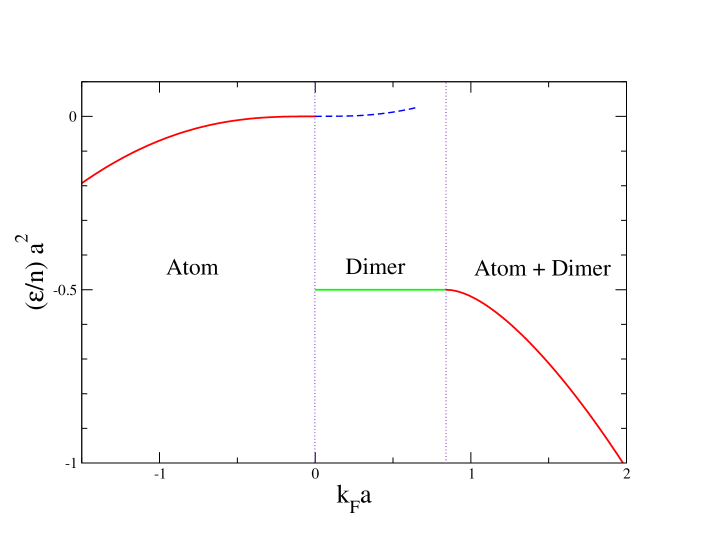
Figure 7: Energy per particle ${\cal E}/n$ in units of $1/a^{2}$ as functions of $k_{F}a$, where $k_{F}=(6\pi^{2}n)^{1/3}$. The vertical dotted lines separate the regions of $k_{F}a$ in which the static homogeneous state includes an atom condensate $(a<0)$, a dimer condensate $(0<a<a_{c})$, and a mixture of atom and dimer condensates $(a>a_{c})$. The dashed line represents an unstable homogeneous state that includes an atom condensate.

The energy density in the static homogeneous state is ${\cal E}={\cal F}+\mu n$, where $\mu$, $n$, and ${\cal F}$ are given in Eqs. (49) and (52). The average energy per atom is

$${\cal E}/n=-{r^{2}(3r-2)\over 2(5r-4)a^{2}}.$$ (56)

The energy per atom is shown as a function of $a$ in Fig. 7. In the high-density limit, a convenient energy scale is the Fermi energy $\epsilon_{F}$ for an ideal gas of fermions with a single spin component: $\epsilon_{F}=\mbox{$\frac{1}{2}$}(6\pi^{2}n)^{2/3}$. The energy per atom in Eqs. (56) has a well-defined unitary limit as $a\to\pm\infty$ with $n$ fixed:

$${\cal E}/n\longrightarrow-\frac{3}{5}\left(\frac{16}{15\pi}\right)^{2/3}\epsilon_{F}\equiv\epsilon_{\infty}.$$ (57)

Its numerical value is $\epsilon_{\infty}\approx-0.292\ \epsilon_{F}.$ If $a<0$, ${\cal E}/n$ decreases from $2\pi na$ to $\epsilon_{\infty}$ as $n$ increases from $0$ to $\infty$. The limiting value $2\pi na$ as $n\to 0$ is the analytic continuation to negative $a$ of the energy per particle of a weakly interacting Bose gas. If $a>0$, ${\cal E}/n$ decreases from $-1/(2a^{2})$ to $\epsilon_{\infty}$ as $n$ increases from $n_{c}$ to $\infty$. The limiting value $-1/(2a^{2})$ at $n=n_{c}$ is the energy per atom for a pair of atoms bound into a dimer with binding energy $E_{D}=1/a^{2}$.

If $a>0$ and $0<n<n_{c}$, there are unphysical solutions to Eqs. (47) and (51a). The expression for $n$ in Eq. (52a) is a cubic polynomial in $r$. It therefore has three roots: a real root in the range ${4\over 5}<r<1$ and a pair of complex roots. For the real root, the expression for $|\bar{A}|^{2}$ in Eq. (50) has an unphysical negative value. For the complex roots, the expression for $|\bar{A}|^{2}$ in Eq. (50) has an unphysical imaginary part. If $n\ll n_{c}$, the complex roots can be expanded in powers of $na^{3}$:

$$r = \pm i(8\pi na^{3})^{1/2}\left[1\pm i\mbox{$5\over 8$}(8\pi na^{3})^{1/2}+\ldots\right].$$ (58)

The thermodynamic quantities corresponding to this root can also be expanded in powers of $na^{3}$. The expansion for the energy per atom is

$${\cal E}/n=2\pi na\left[1\pm i(8\pi na^{3})^{1/2}+\ldots\right].$$ (59)

The leading term in Eq. (59) is the well-known result for the weakly-interacting Bose gas. If $na^{3}$ is small, the imaginary part is suppressed by a factor of $(na^{3})^{1/2}$. If $a$ is decreased through $0$ to a negative value, one of the roots in Eq. (58) becomes the negative value of $r$ that corresponds to the static homogeneous state with mean-field $\bar{A}$ satisfying Eq. (50). Thus the weakly-interacting Bose gas can be interpreted as the analytic continuation to $a>0$ of the static homogeneous state for $a<0$. The real part of ${\cal E}/n$ as a function of $a$ is shown as a dashed line in Fig. 7.

IV.2 Mixture of atom and dimer condensates

If $a>0$, we can also study the static homogeneous states of the system using the truncated 1PI effective action $\Gamma_{1+2}[A,D;\mu]$ given in Eq. (34). In a static homogeneous state, the classical atom and dimer fields must be complex constants: $A({\bf r},t)=\bar{A}$, $D({\bf r},t)=\bar{D}$. We will refer to $\bar{A}$ and $\bar{D}$ as the atom and dimer mean fields, respectively. A state with $\bar{A}\neq 0$ and $\bar{D}\neq 0$ contains a mixture of Bose-Einstein condensates of atoms and dimers. In such a state, a macroscopic fraction $|\bar{A}|^{2}/n$ of the atoms have the same constant wavefunction whose phase is that of $\bar{A}$. A macroscopic fraction $2|\bar{D}|^{2}/n$ of the atoms are bound into dimers that have the same constant center-of-mass wavefunction whose phase is that of $\bar{D}$.

The atom and dimer mean fields $\bar{A}$ and $\bar{D}$ must satisfy Eqs. (35), which reduce to

$$\mu\bar{A} = {16\pi\over ag}\bar{A}^{*}\bar{D}-\frac{4\pi a}{1+r}|\bar{A}|^{2}\bar{A},$$ (60a)

$$2\mu\bar{D} = -{1\over a^{2}}\bar{D}+\mbox{$1\over 2$}g\bar{A}^{2},$$ (60b)

where $r$ is the dimensionless chemical potential variable defined in Eq. (48). Eq. (60b) can be solved for the mean field $\bar{D}$ as a function of $\bar{A}$:

$$\bar{D}=-{ga^{2}\over 2(r^{2}-1)}\bar{A}^{2}.$$ (61)

Inserting this expression for $\bar{D}$ into Eq. (60a) and solving for $|\bar{A}|^{2}$, we obtain the same expression as in Eq. (50), which was derived from the action $\Gamma_{1+2}[A;\mu]$.

The number density $n$ and the free energy density $\cal F$ in the static homogeneous state are given by Eqs. (37) and (39):

$$n = |\bar{A}|^{2}+2|\bar{D}|^{2}+{2\pi a^{3}\over r(r+1)^{2}}|\bar{A}|^{4},$$ (62a)

$${\cal F} = {r^{2}\over 2a^{2}}|\bar{A}|^{2}+{r^{2}-1\over a^{2}}|\bar{D}|^{2}+g\,{\rm Re}(\bar{D}^{*}\bar{A}^{2})-{2\pi a\over r+1}|\bar{A}|^{4}.$$ (62b)

The first two terms in $n$ and in ${\cal F}$ can be interpreted as atom condensate and dimer condensate contributions, respectively. The remaining terms can be interpreted as non-condensate contributions. Using Eqs. (61) and (50) to eliminate the mean fields $\bar{D}$ and $\bar{A}$ in favor of $r$ and $a$, we obtain the same expressions for $n$ and $\cal F$ as in Eqs. (52), which were derived from the action $\Gamma_{1+2}[A;\mu]$.

Nonzero values of $\bar{A}$ and $\bar{D}$ that satisfy the variational equations for $\Gamma_{1+2}[A,D;\mu]$ correspond to a state that contains a mixture of an atom condensate and a dimer condensate. One might be tempted to interpret a nonzero value of $\bar{A}$ that satisfies the variational equations for $\Gamma_{1+2}[A;\mu]$ as the atom mean field in a state with an atom condensate but no dimer condensate. In this case it would seem quite remarkable that the static homogeneous state with nonzero $\bar{A}$ and $\bar{D}$ derived from $\Gamma_{1+2}[A,D;\mu]$ has exactly the same thermodynamic properties as the static homogeneous state with the same value of $\bar{A}$ derived from $\Gamma_{1+2}[A;\mu]$. However the functionals $\Gamma_{1+2}[A;\mu]$ and $\Gamma_{1+2}[A,D;\mu]$ are equivalent. Thus the state with nonzero $\bar{A}$ and $\bar{D}$ derived from $\Gamma_{1+2}[A,D;\mu]$ is in fact identical to the state with the same value of $\bar{A}$ derived from $\Gamma_{1+2}[A;\mu]$. Constructing the equivalent action $\Gamma_{1+2}[A,D;\mu]$ and looking for solutions with a nonzero value of $\bar{D}$ as well as a nonzero value of $\bar{A}$ does not reveal any new states of the system. However it does allow non-atom-condensate contributions to thermodynamic quantities to be resolved into dimer condensate contributions and contributions that correspond to neither atom nor dimer condensates.

Using Eqs. (61), (50), and (52a), we can determine the fraction of the atoms that are in the dimer condensate:

$$2|\bar{D}|^{2}/n=\frac{4r^{2}}{(r+1)^{2}(5r-4)}.$$ (63)

This fraction decreases from $1$ at $n=n_{c}$ to $0$ as $n\to\infty$.

IV.3 Dimer condensate

If $a>0$, we have found that for number density $n$ less than the critical value $n_{c}$ defined in Eq. (53), there are no static homogeneous states with $\bar{A}\neq 0$. However, there is another possibility. If the chemical potential has the value

$$\mu=-1/(2a^{2}),$$ (64)

the variational Eqs. (60) can be satisfied if $\bar{A}=0$ and $\bar{D}\not=0$. This corresponds to a state that has a dimer condensate but no atom condensate. Since $r=1$, the number density and the free energy density in Eqs. (62) reduce to

$$n = 2|\bar{D}|^{2},$$ (65a)

$${\cal F} = 0.$$ (65b)

The energy density is therefore ${\cal E}=\mu n$, and the average energy per atom is

$${\cal E}/n=-1/(2a^{2}).$$ (66)

The energy per atom in this state is shown as a horizontal line in Fig. 7. Since the number density of dimers is $n/2$, the energy per dimer is $-1/a^{2}$. Both $\mu$ and ${\cal E}/n$ have the same values as a gas consisting of dimers that have the binding energy $E_{D}=1/a^{2}$ but are otherwise noninteracting. Thus we can interpret this state as a pure dimer condensate.

IV.4 Discussion of phases

The truncated 1PI approximation predicts one static homogeneous state for any value of the scattering length $a$. We can interpret the various static homogeneous states as different superfluid phases separated by phase transitions at $a=0$ and at the critical value $a=a_{c}$ defined in Eq. (54):

• an atom superfluid phase with only an atom condensate for $-\infty<a<0$,

• a dimer superfluid phase with only a dimer condensate for $0<a<a_{c}$,

• an atom superfluid phase with a mixture of atom and dimer condensates for $a_{c}<a<+\infty$.

The phase transitions are illustrated in Fig. 7, which shows the average energy per atom ${\cal E}/n$ as a function of the dimensionless variable $k_{F}a$, where $k_{F}=(6\pi^{2}n)^{1/3}$ is the Fermi wavenumber of a system of fermions with a single spin state and number density $n$. The energy per particle is given by Eq. (56) for $-\infty<a<0$, by Eq. (66) for $0<a<a_{c}$, and by Eq. (56) again for $a_{c}<a<+\infty$. The energy per particle is discontinuous at $a=0$ and its second derivative is discontinuous at $a=a_{c}$.

We proceed to determine the prediction of the truncated 1PI effective action for the orders of the two phase transitions. The free energy density $\cal F$ is given by Eq. (52b) for $-\infty<a<0$, by Eq. (65b) for $0<a<a_{c}$, and by Eq. (52b) again for $a_{c}<a<+\infty$. The limiting behavior of $\cal F$ in the atom superfluid phase as $a$ approaches the phase transition at $a=0$ is

$${\cal F}\longrightarrow-2\pi an^{2}\qquad{\rm as}\>a\to 0^{-}.$$ (67)

Since ${\cal F}=0$ in the dimer superfluid phase, ${\cal F}$ is continuous at $a=0$ but its first derivative with respect to $a$ is discontinuous. Thus the phase transition at $a=0$ is predicted to be first order. The limiting behavior of $\cal F$ in the atom superfluid phase as $a$ approaches the phase transition at $a=a_{c}$ is

$${\cal F}\longrightarrow\frac{96\pi}{7}n^{2}(a-a_{c})\qquad{\rm as}\>a\to a_{c}^{+}.$$ (68)

Since ${\cal F}=0$ in the dimer superfluid phase, ${\cal F}$ is continuous at $a=a_{c}$ but its first derivative with respect to $a$ is discontinuous. Thus the phase transition at $a=a_{c}$ is also predicted to be first order.

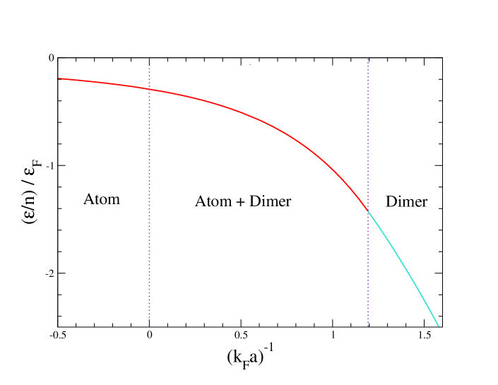
Figure 8: Energy per particle ${\cal E}/n$ in units of the Fermi energy $\epsilon_{F}=k_{F}^{2}/2$ as functions of $(k_{F}a)^{-1}$, where $k_{F}=(6\pi^{2}n)^{1/3}$. The vertical dotted lines separate the regions of $(k_{F}a)^{-1}$ in which the static homogeneous state includes an atom condensate $(a^{-1}<0)$, a mixture of atom and dimer condensates $(0<a^{-1}<a_{c}^{-1})$, and a dimer condensate $(a^{-1}>a_{c}^{-1})$.

The free energy density in Eq. (52b) has the same limiting behavior as $a\to+\infty$ and $a\to-\infty$, so it has a well-behaved unitary limit:

$${\cal F}\longrightarrow\frac{(32\pi/5)^{2/3}}{5}n^{5/3}\qquad{\rm as}\>a\to\pm\infty.$$ (69)

Not only is ${\cal F}$ a continuous function of $a^{-1}$ at $a^{-1}=0$, but all derivatives of ${\cal F}$ with respect to $a^{-1}$ are also continuous. Thus there is no phase transition at $a^{-1}=0$ between the atom superfluid phase for $a^{-1}<0$ and the atom superfluid phase for $a^{-1}>0$. The system in these two regions differs in that there is a dimer condensate for $a^{-1}>0$ and no dimer condensate for $a^{-1}<0$. However the fraction of atoms in the dimer condensate goes to 0 in the unitary limit in such a way that all thermodynamic variables remain smooth. The smooth behavior of the energy per atom as a function of $a^{-1}$ at $a^{-1}=0$ is illustrated in Fig. 8.

The smooth behavior of the thermodynamic variables at $a^{-1}=0$ is consistent with the universality hypothesis proposed by Ho Ho-2004-92 , which asserts that the thermodynamic properties of the system in the unitary limit $a=\pm\infty$ are universal functions of the number density $n$ and the temperature $T$ and don’t depend on any interaction parameters. This hypothesis requires that a thermodynamic variable at $T=0$ and $a=\pm\infty$ have the form $A\ n^{p}$, where $A$ is a constant and $p$ is the power required by dimensional analysis. This hypothesis is well established for systems consisting of fermions with two spin states. Ho proposed that it might also apply to bosonic systems.

If a many-body system consisting of identical bosons with large scattering length $a$ has number density $n$ and temperature $T$ such that $n^{-1/3}$ and $(mT/\hbar^{2})^{-1/2}$ are large compared to the range, its behavior should be determined by $a$ and the Efimov parameter $\kappa_{*}$ and it should be governed by the discrete scaling symmetry. Efimov physics requires a modification of Ho’s universality hypothesis Ho-2004-92 to allow for log-periodic dependence on the Efimov parameter $\kappa_{*}$. For example, a thermodynamic variable at zero temperature in the unitary limit $a=\pm\infty$ must have the form $n^{p}\ f(s_{0}\log(n/\kappa_{*}^{3}))$, where $p$ is the power required by dimensional analysis and $f(\theta)$ is a dimensionless function with period $2\pi$. Our truncated 1PI approximation does not give this behavior, because irreducible 3-body amplitudes have been neglected.

IV.5 Comparison with previous work

Several groups have studied the static homogeneous states for the many-body system of bosonic atoms near a Feshbach resonance  RPW ; RDSS ; LL ; BM . The starting point for all these analyses could be taken to be the quantum field theory with an atom field $\hat{\psi}_{A}({\bf r},t)$ and a molecule field $\hat{\psi}_{M}({\bf r},t)$ defined by the Hamiltonian density in Eq. (7). They considered the phase diagram of the system as a function of the atom number density $n$, the temperature $T$, and a detuning variable that determines the scattering length $a$ of the atoms. When the scattering length is large compared to all other length scales, the low energy behavior of the system should be the same as in the zero-range model. We can compare our results from the truncated 1PI effective action at zero temperature with their results for large scattering length.

We first consider the qualitative behavior of the phase diagram at $T=0$. Radzihovsky, Park and Weichman (RPW) and Romans, Duine, Sachdev and Stoof (RDSS) independently pointed out that this system has a quantum phase transition between an atom superfluid phase and a molecular superfluid phase RPW ; RDSS . The quantum phase transition is between states with different symmetries. The fundamental theory defined by the Hamiltonian density in Eq. (7) has a $U(1)$ symmetry corresponding to phase transformations of the atom and molecule quantum fields: $\hat{\psi}_{A}\to e^{i\theta}\hat{\psi}_{A}$, $\hat{\psi}_{M}\to e^{2i\theta}\hat{\psi}_{M}$. In the atom superfluid phase, both the atom and molecule fields have nonzero expectation values $\langle\hat{\psi}_{A}\rangle$ and $\langle\hat{\psi}_{M}\rangle$, so the $U(1)$ symmetry is completely broken to the trivial subgroup $\{+1\}$. In the molecular superfluid phase, $\langle\hat{\psi}_{M}\rangle$ is nonzero but $\langle\hat{\psi}_{A}\rangle=0$, so the $U(1)$ symmetry is broken to the subgroup $Z_{2}=\{+1,-1\}$. Thus the order parameter for the phase transition is an element of the discrete group $Z_{2}$ RPW ; RDSS . For $a>0$, the classical atom and dimer fields $A$ and $D$ in the truncated 1PI effective action $\Gamma_{1+2}[A,D;\mu]$ play the same role as the expectation values $\langle\hat{\psi}_{A}\rangle$ and $\langle\hat{\psi}_{M}\rangle$ in Refs. RPW ; RDSS . For $a<0$, we have no analog of $\langle\hat{\psi}_{M}\rangle$. However the classical atom field $A$ in the truncated 1PI effective action $\Gamma_{1+2}[A;\mu]$ plays the same role as the expectation value $\langle\hat{\psi}_{A}\rangle$ in Refs. RPW ; RDSS .

The order of the quantum phase transition between the atom superfluid phase and the molecular superfluid phase has been discussed in Refs. RPW ; RDSS ; LL . Because the two phases are distinguished by a $Z_{2}$ order parameter, one might expect the phase transition to be in the universality class of the $4$-dimensional Ising model, which has a second order transition. However, the coupling of the $Z_{2}$ order parameter to the Goldstone mode associated with the molecule condensate phase modifies the critical behavior and makes the phase transition weakly first order. The mean-field approximation predicts that the phase transition is second order. Lee and Lee used the renormalization group to show that the phase transition is first order LL . The truncated 1PI approximation correctly predicts that the phase transition is first order.

The analysis of the static homogeneous states by RPW RPW was carried out using the mean-field approximation, in which the quantum field operators in Eq. (7) are replaced by classical fields $\psi_{A}({\bf r},t)$ and $\psi_{M}({\bf r},t)$ and the bare parameters, which depend on the ultraviolet cutoff $\Lambda$, are replaced by mean-field parameters. The analysis of the static homogeneous states by RDSS RDSS included some effects that go beyond the mean-field approximation. The grand Hamiltonian density in the mean-field approximation is

$${\cal H}-\mu n = \psi_{A}^{*}\left(-\mbox{$\frac{1}{2}$}\nabla^{2}-\mu\right)\psi_{A}\,+\,\psi_{M}^{*}\left(-\mbox{$\frac{1}{4}$}\nabla^{2}-2\mu+\nu_{M}\right)\psi_{M}$$ (70)

$$+ \mbox{$\frac{1}{4}$}\lambda_{AA}\left(\psi_{A}^{*}\psi_{A}\right)^{2}\,+\,\mbox{$\frac{1}{2}$}g_{AM}\left(\psi_{A}^{*2}\psi_{M}+\psi_{M}^{*}\psi_{A}^{2}\right)$$

$$+ \lambda_{AM}\psi_{M}^{*}\psi_{A}^{*}\psi_{A}\psi_{M}\,+\,\mbox{$\frac{1}{4}$}\lambda_{MM}\left(\psi_{M}^{*}\psi_{M}\right)^{2}.$$

The mean-field predictions for the scattering observables are sums of tree diagrams whose vertices are given by the interaction terms in Eq. (70). For example, the $T$-matrix element for atom-atom scattering is given by the sum of the two diagrams in Fig. 5, where the vertices in the first diagram are $-ig_{AM}$ and the vertex in the second diagram is $-i\lambda_{AA}$. The resulting expression for the scattering length is

$$a=\frac{1}{8\pi}\left(\lambda_{AA}-\frac{g_{AM}^{2}}{\nu_{M}}\right).$$ (71)

The resonance where the scattering length $a$ diverges is reached by tuning the parameter $\nu_{M}$ to 0.

We first discuss the values of the mean-field parameters in Ref. RPW . RPW stated that in the dilute gas limit, $\lambda_{AA}$, $\lambda_{AM}$, $\lambda_{MM}$ are proportional to the scattering lengths for atom-atom, atom-molecule, and molecule-molecule scattering, respectively. This presumably means that the scattering length $a$ is given by Eq. (71) with $g_{AM}=0$. This would be inconsistent with the classical approximation. RPW did not specify the parameter $g_{AM}$. They also did not discuss the behavior of the mean-field parameters near the resonance where the scattering length $a$ is large.

The approximations of RDSS can also be expressed in terms of an effective Hamiltonian with the terms in Eq. (70) RDSS . They discussed the behavior of the mean-field parameters near the resonance where $a\to+\infty$. For $a>0$, which corresponds to negative detuning, the limiting behavior of the parameters is

$$\nu_{M} \longrightarrow -1/a^{2},$$ (72a)

$$g_{AM} \longrightarrow \sqrt{16\pi/a},$$ (72b)

$$\lambda_{AA} = 8\pi a_{bg},$$ (72c)

$$\lambda_{AM} \longrightarrow 32\pi a,$$ (72d)

$$\lambda_{MM} \longrightarrow 16\pi a.$$ (72e)

The limiting behavior of the detuning parameter $\nu_{M}$ is the energy of the weakly-bound dimer. The limiting value of $g_{AM}$ also comes from the exact solution of the 2-body problem. Note that all the coefficients in Eqs. (72) scale as powers of $a$ except $\lambda_{AA}$. RDSS took $\lambda_{AA}$ to be a constant, so it gives a non-resonant contribution $a_{bg}$ to the scattering length in Eq. (71). Note that if the limiting values of $\nu_{M}$, $\lambda_{AA}$, and $g_{AM}$ in Eqs. (72) are inserted into the right side of Eq. (71), the limiting value is $2a$ instead of $a$. RDSS took $\lambda_{AM}$ and $\lambda_{MM}$ to be proportional to the scattering lengths for atom-molecule and molecule-molecule scattering. They recognized that in the limit $a\to\infty$, these scattering lengths must scale linearly with the large scattering length $a$. RDSS did not recognize that Efimov physics requires the coefficients of $a$ in these scattering lengths to be log-periodic functions of $a$ of the form $f(s_{0}\log(a\kappa_{*}))$, where $\kappa_{*}$ is the Efimov parameter and $f(\theta)$ is a function with period $2\pi$. They calculated the atom-dimer and dimer-dimer scattering lengths using an approximation in which 2-body quantum effects are treated exactly, the atom-dimer coupling constant $g_{AM}$ is treated as a perturbation, and other irreducible 3-body and 4-body quantum effects are neglected. In the case of the atom-dimer scattering length $a_{AD}$, this approximation is equivalent to our truncated 1PI approximation. Their result for $a_{AD}$ differs from ours in Eq. (41) by a factor of $-2$. Both results for $a_{AD}$ differ from the exact result in Eq. (45) in which the coefficient of $a$ is a log-periodic function of $a\kappa_{*}$. The approximation of RDSS for the dimer-dimer scattering length is $a_{DD}=4a$. The exact result for $a_{DD}$ has not yet been calculated.

Our truncated 1PI approximation gives predictions for the parameters in the mean-field Hamiltonian in Eq. (70) in the limit of large scattering length. The classical atom field $A({\bf r},t)$ in the 1PI effective action can be naturally identified with the atom mean field $\psi_{A}({\bf r},t)$. If $a>0$, we can also identify the classical dimer field $D({\bf r},t)$ with the molecular mean field $\psi_{M}({\bf r},t)$. Inserting constant mean fields $\bar{A}$ and $\bar{D}$ into the truncated 1PI effective action in Eq. (34), it reduces to

$$\Gamma_{1+2}[{\bar{A}},{\bar{D}};\mu] = \int dt\int d^{3}r\left\{\mu{\bar{A}}^{*}{\bar{A}}+\left(2\mu+1/a^{2}\right){\bar{D}}^{*}{\bar{D}}\right.$$ (73)

$$\hskip 56.9055pt\left.-\sqrt{4\pi/a}\left({\bar{A}}^{*2}{\bar{D}}+{\bar{D}}^{*}{\bar{A}}^{2}\right)+\frac{2\pi a}{1+a\sqrt{-2\mu}}\left({\bar{A}}^{*}{\bar{A}}\right)^{2}\right\}.$$

We can identify the integrand with the negative of the Hamiltonian density in Eq. (70) for constant values of the mean fields $\psi_{A}$ and $\psi_{M}$. The resulting predictions for the mean-field parameters associated with 2-atom terms are

$$\nu_{M} = -1/a^{2},$$ (74a)

$$g_{AM} = \sqrt{16\pi/a},$$ (74b)

$$\lambda_{AA} = \frac{-8\pi a}{1+a\sqrt{-2\mu}}.$$ (74c)

The values of $\nu_{M}$ and $g_{AM}$ agree with the limiting values of RDSS near the Feshbach resonance. Note that the value of $\lambda_{AA}$ depends on the chemical potential, which depends on the number density. If we take the dilute limit in which $\mu\to 0$ and insert the parameters in Eq. (74) into the right side of Eq. (71), we get the correct scattering length $a$. Note that the scattering length is obtained as the sum of two terms: $a=(-a)+2a$.

A comparison of Eqs. (70) and (73) shows that the truncated 1PI approximation predicts $\lambda_{AM}=0$ and $\lambda_{MM}=0$. These predictions are artifacts of our truncation of the 1PI effective action after the 2-atom terms. If the 1PI effective actions were truncated after the 3-atom terms, there would be an additional term $\lambda_{AM}{\bar{D}}^{*}{\bar{A}}^{*}{\bar{A}}{\bar{D}}$ in Eq. (73). If it were truncated after the 4-atom terms, there would also be a term $\mbox{$\frac{1}{4}$}\lambda_{MM}({\bar{D}}^{*}{\bar{D}})^{2}$. Using the exact result for the atom-dimer scattering length $a_{AD}$ in Eq. (45), we can deduce the value of $\lambda_{AM}$. The $T$-matrix element $i{\cal T}$ for atom-dimer scattering is the sum of tree diagrams whose vertices are 1PI amplitudes. Thus it is the sum of the diagram in Fig. 6 whose contribution to the $T$-matrix element is given in Eq. (40) and a diagram with a 1PI atom-dimer scattering amplitude. For zero collision energy, the 1PI atom-dimer scattering diagram reduces to $-i\lambda_{AM}$ and the $T$-matrix element reduces to ${\cal T}=-3\pi a_{AD}$. Thus the atom-dimer scattering length is

$$a_{AD}=\frac{\lambda_{AM}}{3\pi}-\frac{16}{3}a.$$ (75)

Comparing with the exact result for $a_{AD}$ in Eq. (45), we obtain the exact result for $\lambda_{AM}$:

$$\lambda_{AM}=3\pi\big{(}6.79-2.15\tan\left[s_{0}\ln(a\kappa_{*})+1.16\right]\big{)}\ a,$$ (76)

where $s_{0}=1.00624$ and $\kappa_{*}$ is the Efimov parameter.

The location of the quantum phase transition in the mean-field approximation was determined in RPW and RDSS RPW ; RDSS . The critical number density $n_{c}$ at the quantum phase transition satisfies

$$\nu_{M}=-g_{AM}\sqrt{2n_{c}}+\left(\lambda_{AM}-\mbox{$\frac{1}{4}$}\lambda_{MM}\right)n_{c}.$$ (77)

If the dependence of the mean-field parameters on the detuning parameter, or equivalently, on the scattering length $a$, is known, this condition can be translated into a critical value $a_{c}$ of the scattering length. To compare the condition in Eq. (77) with the results from the truncated 1PI effective action, we must set $\lambda_{AM}=\lambda_{MM}=0$. Using the values of $\nu_{M}$ and $g_{AM}$ in Eq. (74), we recover the expression for the critical number density $n_{c}$ in Eq. (53).

V Quasiparticles

In this section, we use the truncated 1PI approximation to study the quasiparticles associated with small fluctuations around the static homogeneous states. There are two types of quasiparticles: atom quasiparticles with dispersion relation $\omega_{A}(k)$ and pair quasiparticles with dispersion relation $\omega_{P}(k)$. The two types of quasiparticles can be distinguished by whether the asymptotic behavior of their dispersion relations as $k\to\infty$ is that for an atom or a pair of atoms:

$$\omega_{A}(k) \longrightarrow\mbox{$\frac{1}{2}$}k^{2},$$ (78a)

$$\omega_{P}(k) \longrightarrow\mbox{$\frac{1}{4}$}k^{2}.$$ (78b)

If the dispersion relation $\omega(k)$ for a quasiparticle has an imaginary part, it indicates a dynamical instability of the system.

V.1 Atom condensate

To find the dispersion relation $\omega(k)$ for quasiparticles associated with fluctuations of $A({\bf r},t)$ around the mean-field value $\bar{A}$, we look for solutions to Eq. (30) of the form

$$A({\bf r},t)=\bar{A}+\tilde{A}_{+}e^{-i\omega t+i{\bf k}\cdot{\bf r}}+\tilde{A}_{-}e^{+i\omega t-i{\bf k}\cdot{\bf r}},$$ (79)

with $\tilde{A}_{+}$ and $\tilde{A}_{-}$ infinitesimal. There are nontrivial solutions for $\tilde{A}_{+}$ and $\tilde{A}_{-}$ only if the dispersion relations $\omega(k)$ satisfy

$$0 = (a^{2}\omega)^{2}+r^{2}(r-1)[f_{+}-f_{-}]a^{2}\omega-\mbox{$1\over 2$}r^{2}(r-1)[f_{+}+f_{-}](r^{2}+a^{2}k^{2})$$ (80)

$$-r^{4}(r-1)^{2}f_{+}f_{-}-\mbox{$1\over 4$}a^{2}k^{2}(2r^{2}+a^{2}k^{2}),$$

where

$$f_{\pm}={1\over 1-r(1+{1\over 4}a^{2}k^{2}/r^{2}\pm a^{2}\omega/r^{2}-i\epsilon)^{1/2}}\ .$$ (81)

Since Eq. (80) is even in $\omega$, the solutions come in pairs: if $\omega(k)$ is a solution, so is $-\omega(k)$. The invariance of $\Gamma[A]$ under the $U(1)$ phase symmetry $A\to e^{i\alpha}A$ guarantees that there must be a solution that satisfies $\omega(k=0)=0$. This can be confirmed by observing that $\omega=k=0$ is indeed a solution to Eq. (80).

Using algebraic manipulations, Eq. (80) can be transformed into a 6^th order polynomial equation in $\omega^{2}$ zhang-thesis . The polynomial equation is extremely complicated, with 266 terms when fully expanded into a polynomial in $\omega$, $k$ and $r$. The explicit form is not very illuminating, so we do not write it down here. It is important that Eq. (80) can be transformed into a polynomial equation, because it guarantees that we can find all the dispersion relations that satisfy Eq. (80). A $6$th order polynomial equation in $\omega^{2}$ has precisely $6$ roots in the complex $\omega^{2}$ plane. Given numerical values of $r$ and $k$, the $6$ roots of the polynomial equation for $\omega^{2}$ can be easily found numerically. One can then substitute the $12$ roots for $\omega$ into Eq. (80) to see which ones correspond to quasiparticle dispersion relations $\omega(k)$.

We proceed to consider various limits in which the quasiparticle dispersion relations that satisfy Eq. (80) can be obtained in closed form.

V.1.1 Non-interacting limit

In the limit $r\to 0^{-}$, the quasiparticle dispersion relations reduce to

$$\omega_{A}(k) = \mbox{$\frac{1}{2}$}k^{2},$$ (82a)

$$\omega_{P}(k) = -1/{a^{2}}+\mbox{$\frac{1}{4}$}k^{2}.$$ (82b)

These are the dispersion relation for an isolated atom and for an isolated dimer with binding energy $E_{D}=1/a^{2}$, respectively. The atom and pair dispersion relations in Eqs. (82) are illustrated in Fig. 9 as dashed lines. Since they are dispersion relations for isolated atoms and dimers, we refer to the limit $r\to 0^{-}$ as the non-interacting limit. Since $\omega_{A}(k)$ and $\omega_{P}(k)$ are real for all $k$, the homogeneous state is dynamically stable in the non-interacting limit.

Figure 9: Atom and pair dispersion relations in the non-interacting limit ($r\to 0^{-}$, dashed line) and the critical density ($r\to 1^{+}$, solid line).

V.1.2 Critical density $n_{c}$

The limit $r\to 1^{+}$ corresponds to the critical density $n_{c}=1/(32\pi a^{3})$ defined in Eq. (53). In this limit, the quasiparticle dispersion relations reduce to

$$\omega_{A}(k) = \mbox{$\frac{1}{2}$}k\left(k^{2}+2/{a^{2}}\right)^{1/2},$$ (83a)

$$\omega_{P}(k) = \mbox{$\frac{1}{4}$}k^{2}.$$ (83b)

The atom dispersion relation is that for the Bogoliubov mode in a superfluid with coherence length $a/\sqrt{2}$. The pair dispersion relation is that for a dimer whose binding energy $E_{D}=1/a^{2}$ is cancelled by its mean field energy. The atom and pair dispersion relations in Eqs. (83) are illustrated in Fig. 9 as solid lines. Since $\omega_{A}(k)$ and $\omega_{P}(k)$ are real for all $k>0$, the homogeneous state is dynamically stable at the critical density.

V.1.3 Unitary limit

The unitary limit is $a\to\pm\infty$ with fixed number density $n$. It corresponds to $r\to\pm\infty$ with $r/a=\sqrt{-2\mu}$ fixed. In this limit, it is convenient to introduce dimensionless scaling variables for the frequency and wavenumber: $\hat{\omega}=\omega a^{2}/r^{2}$, $\hat{k}=ka/r$. After multiplying Eq. (80) by $r^{-4}$ and taking the limit $r\to\pm\infty$, it reduces to

$$0={\hat{\omega}}^{2}+({\hat{f}}_{+}-{\hat{f}}_{-}){\hat{\omega}}-\mbox{$\frac{1}{2}$}({\hat{f}}_{+}+{\hat{f}}_{-})(1+{\hat{k}}^{2})-{\hat{f}}_{+}{\hat{f}}_{-}-\mbox{$\frac{1}{4}$}{\hat{k}}^{2}(2+{\hat{k}}^{2}),$$ (84)

where

$${\hat{f}}_{\pm}=\frac{-1}{(1+{1\over 4}{\hat{k}}^{2}\pm{\hat{\omega}}-i\epsilon)^{1/2}}.$$ (85)

Using algebraic manipulations, Eq. (84) can be transformed into a 6^th order polynomial equation in $\hat{\omega}^{2}$ zhang-thesis . The solutions must be inserted into Eq. (84) to find which ones are quasiparticle dispersion relations. The atom and pair dispersion relations at large $\hat{k}$ have expansions in powers of $1/\hat{k}$:

$$\hat{\omega}_{A}(k) = \frac{1}{2}\hat{k}^{2}+\frac{1}{2}\pm i\frac{2}{\hat{k}}+\ldots,$$ (86a)

$$\hat{\omega}_{P}(k) = \frac{1}{4}\hat{k}^{2}+1-\frac{16}{\hat{k}^{4}}+\ldots$$ (86b)

The sign of the imaginary part of $\hat{\omega}_{A}(k)$ is determined by the choice of branch cut for the square root in Eq. (85). The terms of order $\hat{k}^{0}$ in Eqs. (86) imply that the atom and dimer have mean-field energies $|\mu|$ and $2|\mu|$, respectively. The limiting behaviors of the dispersion relations as $k\to 0$ are

$$\omega_{A}^{2}(k) \longrightarrow (0.12\pm i\ 0.45)\ k_{F}^{4},$$ (87a)

$$\omega_{P}^{2}(k) \longrightarrow -\mbox{$\frac{1}{3}$}(\mbox{$\frac{32}{5}$}\pi n)^{2/3}\,k^{2},$$ (87b)

where $k_{F}=(6\pi^{2}n)^{1/3}$ is the Fermi wavenumber.

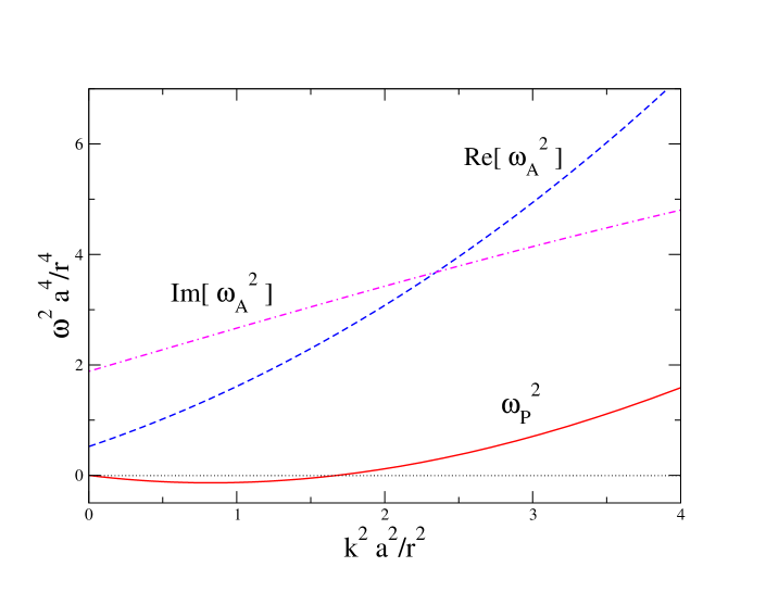
Figure 10: The square of the pair dispersion relation (solid line) and the real and imaginary parts of the square of the atom dispersion relation (dashed line and dash-dotted line) in the unitary limit $a\to\pm\infty$ with $n$ fixed.

The atom and pair dispersion relations in the unitary limit are illustrated in Fig. 10 by plotting ${\rm Re}[\hat{\omega}_{A}^{2}]$, ${\rm Im}[\hat{\omega}_{A}^{2}]$, and $\hat{\omega}_{P}^{2}$ as functions of $\hat{k}^{2}$. The atom dispersion relation $\hat{\omega}_{A}$ is complex valued for all $\hat{k}$. This indicates the system is unstable under fluctuations of any wavelength. The pair dispersion relation $\hat{\omega}_{P}$ remains real until $k$ decreases below the critical value $k_{c}\approx 0.907\,k_{F}$, after which $\hat{\omega}_{P}$ becomes pure imaginary.

V.1.4 General case

Eq. (80) for the quasiparticle dispersion relations cannot be solved analytically for general values of $r$ in the range $-\infty<r<0$ and $1<r<+\infty$. However, analytic expression can be obtained for limiting values of $k$. At large $k$, the atom and pair dispersion relations have expansions in powers of $1/k$:

$$\omega_{A}(k) = \mbox{$\frac{1}{2}$}k^{2}+\frac{r^{2}}{2a^{2}}\pm i\frac{2r^{2}(r-1)}{ka^{3}}+\cdots,$$ (88a)

$$\omega_{P}(k) = \mbox{$\frac{1}{4}$}k^{2}+\frac{r^{2}-1}{a^{2}}-\frac{8r^{2}(r-1)}{k^{2}a^{4}}+\cdots.$$ (88b)

The terms of order $k^{0}$ imply that the atom and pair quasiparticles have mean-field energies $\mbox{$\frac{1}{2}$}r^{2}E_{D}$ and $r^{2}E_{D}$, respectively. Except at the limiting values $r\to 0^{-}$ and $r\to 1^{+}$, the atom dispersion relation $\omega_{A}(k)$ is complex for all $k$. Thus the system is unstable under nonhomogeneous fluctuations with any wavelength. The pair dispersion relation $\omega_{P}(k)$ remains real until $k$ decreases below a critical value $k_{c}$ that satisfies zhang-thesis

$$0=(k_{c}a)^{6}+4(k_{c}a)^{4}(r^{2}-1)-16(k_{c}a)^{2}r^{2}(r-1)-16r^{4}(r-1)^{2},$$ (89)

and then it becomes pure imaginary. As $r$ increases from $1$ to $+\infty$ and then increases from $-\infty$ to 0, $k_{c}$ increases from $0$ to $0.907\,k_{F}$ and then decreases to 0.

V.2 Mixture of atom and dimer condensates

To find the dispersion relations $\omega(k)$ for quasiparticles associated with fluctuations of $A({\bf r},t)$ and $D({\bf r},t)$ around the mean-field values $\bar{A}$ and $\bar{D}$, we look for solutions to Eqs. (35) of the form

$$A({\bf r},t) = \bar{A}+\tilde{A}_{+}e^{-i\omega t+i{\bf k}\cdot{\bf r}}+\tilde{A}_{-}e^{+i\omega t-i{\bf k}\cdot{\bf r}},$$ (90a)

$$D({\bf r},t) = \bar{D}+\tilde{D}_{+}e^{-i\omega t+i{\bf k}\cdot{\bf r}}+\tilde{D}_{-}e^{+i\omega t-i{\bf k}\cdot{\bf r}},$$ (90b)

with $\tilde{A}_{+}$, $\tilde{A}_{-}$, $\tilde{D}_{+}$, and $\tilde{D}_{-}$ infinitesimal. Surprisingly, the condition for non-trivial solutions can be reduced to Eq. (80) zhang-thesis . Thus the dispersion relations for fluctuations of $A({\bf r},t)$ and $D({\bf r},t)$ predicted by Eq. (35) are identical to the dispersion relations for fluctuations of $A({\bf r},t)$ predicted by Eq. (30). This may seem quite remarkable at first, but it is a consequence of the equivalence of the effective actions $\Gamma_{1+2}[A;\mu]$ and $\Gamma_{1+2}[A,D;\mu]$. Although these effective actions give the same dispersion relations, the coefficients of $\tilde{A}_{+}$, $\tilde{A}_{-}$, $\tilde{D}_{+}$, and $\tilde{D}_{-}$ obtained by solving Eq. (35) provide more detailed information about the nature of the quasiparticles than the coefficients of $\tilde{A}_{+}$ and $\tilde{A}_{-}$ obtained by solving Eq. (30).

V.3 Pure dimer condensate

If $a>0$ and $0<n<n_{c}$, the static homogeneous state is a dimer superfluid with mean fields $\bar{D}\neq 0$ and $\bar{A}=0$. The equations for small oscillations of $A({\bf r},t)$ around $0$ and $D({\bf r},t)$ around $\bar{D}$ decouple. The dispersion relations are

$$\omega_{A}(k) = \left[\left(1/(2a^{2})+\mbox{$\frac{1}{2}$}k^{2}\right)^{2}-8\pi n/a\right]^{1/2},$$ (91a)

$$\omega_{P}(k) = \mbox{$\frac{1}{4}$}k^{2}.$$ (91b)

The pair dispersion relation in Eq. (91b) corresponds to a dimer whose binding energy $E_{D}=1/a^{2}$ is exactly canceled by its mean-field energy. The atom dispersion relation in Eq. (91a) corresponds to a mean-field energy $[1/(2a^{2})^{2}-8\pi n/a]^{1/2}$. The mean-field energy vanishes at the critical density $n_{c}=(32\pi a^{3})^{-1}$.

The dispersion relations in Eq. (91) are real-valued for all $k$. Thus if $a>0$, the truncated 1PI approximation predicts that the pure dimer condensate is stable for $n<n_{c}$. The existence of Efimov states suggests that if 3-body effects were taken into account, the static homogeneous state containing a dimer condensate but no atom condensate would also be unstable for $n<n_{c}$. Thus the stability of the dimer superfluid is probably an artifact of the truncated 1PI approximation.

V.4 Comparison with previous work

Several groups have studied the quasiparticle dispersion relations for the many-body system of bosonic atoms near a Feshbach resonance using the mean-field approximation RPW ; RDSS ; BM . RPW and RDSS derived the quasiparticle dispersion relations in the molecular superfluid phase RPW ; RDSS . Their dispersion relations reduce to our results in Eqs. (91) if we set $\lambda_{AM}=\lambda_{MM}=0$ and insert the values of the mean-field parameters for the truncated 1PI approximation given in Eqs. (74). Basu and Mueller studied the quasiparticle dispersion relations in the atom superfluid phase BM . They showed that if the atom-molecule and molecule-molecule coupling constants $\lambda_{AM}$ and $\lambda_{MM}$ are set to zero, there is a dispersion relation with the behavior $\omega^{2}\to c_{s}^{2}k^{2}$ as $k\to 0$ with $c_{s}^{2}<0$. Thus the atom superfluid phase is unstable with respect to long-wavelength fluctuations. Our result for the pair dispersion relation $\omega_{P}(k)$ in the unitary limit in Eq. (87b) is consistent with their result. Our results go further by showing that the atom dispersion relation $\omega_{A}(k)$ is complex for all $k$. Thus the atom superfluid phase is unstable with respect to fluctuations of any wavelength.

VI summary

Previous work on the dimer superfluid phase of the strongly-interacting Bose gas has relied on the existence of a quantum field whose expectation value can indicate the presence of a dimer condensate. The atom superfluid phase and the dimer superfluid phase can both be described using the mean-field approximation. However a dimer condensate is also possible in models when there is no such quantum field. In this case, the mean-field approximation cannot be used to describe the dimer superfluid. We have developed a method for describing the dimer condensate in such case. It is based on the 1PI effective action $\Gamma[A]$, which is a functional of classical atom field $A({\bf r},t)$ that encodes complete quantum information of the system. The solutions to the variational equation for $\Gamma[A]$ correspond to states that contains an atom condensate only or a mixture of an atom condensate and a dimer condensate. The functional $\Gamma[A]$ also contains information about states that contains a dimer condensate but no atom condensate, but it is encoded in a more subtle way through poles in functions of differential operators. In the case $a>0$, we constructed an equivalent 1PI effective action $\Gamma[A,D]$ that is also a functional of a classical dimer field $D({\bf r},t)$. Some of the solutions to the variational equation for $\Gamma[A,D]$ correspond to the same states as the solutions to the variational equation for $\Gamma[A]$. These states contain an atom condensate only or a mixture of an atom condensate and a dimer condensate. However the variational equations for $\Gamma[A,D]$ has additional solutions that correspond to states containing a dimer condensate but no atom condensate.

To illustrate our method for describing the dimer condensate, we introduced an approximation in which 1-atom and 2-atom terms are treated exactly while irreducible $N$-atom terms with $N\geq 3$ are ignored. This approximation can be defined by truncated 1PI effective actions $\Gamma_{1+2}[A]$ and $\Gamma_{1+2}[A,D]$. We determined these functionals exactly for the zero-range model in which the only interaction parameter is the large scattering length $a$. We demonstrated the limitations of the truncated 1PI approximation by using it to calculate the cross section for atom-dimer elastic scattering. We compared the results with those from exact solutions of the 3-body problem, which depend on the Efimov parameter $\kappa_{*}$. The errors can be very large, so the truncated 1PI approximation is not useful as a quantitative approximation. However many results can be obtained analytically in this approximation, so it may be useful as a benchmark against which results from other methods can be compared. We have found the truncated 1PI approximation to be particularly useful for illustrating applications of the 1PI effective action.

We applied the truncated 1PI approximation to the homogeneous strongly-interacting Bose gas at zero temperature. We first determined the static homogeneous states of the system. The phase diagram is qualitatively consistent with that derived in Refs. RPW ; RDSS . There is an atom superfluid phase and a dimer superfluid phase separated by quantum phase transitions at $a=0$ and $a_{c}=(32\pi n)^{-1/3}$. The unitary limit $a\to\pm\infty$ is consistent with Ho’s universality hypothesis Ho-2004-92 . There is a perfectly smooth transition from an atom superfluid state containing a mixture of an atom condensate and a dimer condensate as $a\to+\infty$ to an atom superfluid containing an atom condensate only as $a\to-\infty$. We also determined the quasiparticles dispersion relations associated with small fluctuations around the homogeneous states. In the atom superfluid state, the pair dispersion relation $\omega_{P}(k)$ is pure imaginary for sufficiently small $k$, indicating an instability with respect to long-wavelength fluctuations. The atom dispersion relation $\omega_{A}(k)$ is complex for all $k$, indicating an instability with respect to fluctuations of any wavelength. In the dimer superfluid state, the atom and pair dispersion relations are real-valued for all $k$, indicating that the system is dynamically stable. We suggested that this stability is an artifact of the truncated 1PI approximation. In the case $a>0$, the properties of the atom superfluid phase could be derived either from the variational equation for $\Gamma_{1+2}[A]$ or from the variational equations for $\Gamma_{1+2}[A,D]$. They give exactly the same thermodynamic properties and identical quasiparticle dispersion relations. This illustrates the equivalence of these two truncated 1PI effective actions. Some advantages of $\Gamma_{1+2}[A,D]$ are that it allows the non-condensate contributions to thermodynamic properties to be separated into a dimer-condensate contribution and a remainder and it gives more detailed information about the nature of the quasiparticles. The properties of the dimer superfluid phase can be derived easily from the variational equations for $\Gamma_{1+2}[A,D]$. That information must also be encoded in $\Gamma_{1+2}[A]$, since these two functional are equivalent, but is is in a much less accessible form.

Much of the previous work on the Bose gas near a Feshbach resonance has been carried out with the mean-field approximation using the Hamiltonian density in Eq. (70), which depends on atomic and molecular mean fields $\psi_{A}$ and $\psi_{M}$. We used the truncated 1PI effective action $\Gamma_{1+2}[A,D]$ to deduce the limiting values of some of the mean-field parameters when the system is sufficiently close enough to the Feshbach resonance. Our results for $\nu_{M}$ and $g_{AM}$ agree with those of Ref. RDSS . Our result for $\lambda_{AA}$ increases linearly with $a$, while $\lambda_{AA}$ was assumed to be constant in Ref. RDSS . We also used results from exact solutions to the 3-body problem to deduce the limiting value of $\lambda_{AM}$. Our result for $\lambda_{AM}$ in Eq. (76) has log-periodic dependence on the Efimov parameter. The simple result $\lambda_{AM}\to 32\pi a$ in Ref. RDSS was derived using an approximation equivalent to the truncated 1PI approximation.

The method we have used to describe states containing a dimer condensate can be generalized to states containing condensates of Efimov trimers. Information about a specific Efimov trimer is encoded in the 1PI effective action $\Gamma[A]$ through the poles of functions of differential operators that act on products of three classical atom fields. By introducing a classical trimer field $T({\bf r},t)$, it should be possible to construct an equivalent 1PI effective action $\Gamma[A,T]$ or $\Gamma[A,D,T]$ in which these poles have been eliminated. One could then use the variational equation for these effective actions to study the trimer superfluid phase of the strongly-interacting Bose gas.

- (1) M. H. Anderson et al, Science 269, 198-201 (1995).
- (2) K. B. Davis et al, Phys. Rev. Lett. 75, 3969 (1995).
- (3) C. C. Bradley et al, Phys. Rev. Lett. 75, 1687 (1995).
- (4) S. Inouye, M.R. Andrews, J. Stenger, H.-J. Miesner, D.M. Stamper-Kurn, and W. Ketterle, Nature 392, 151 (1998).
- (5) Ph. Courteille, R.S. Freeland, D.J. Heinzen, F.A. van Abeelen, and B.J. Verhaar, Phys. Rev. Lett. 81, 69 (1998).
- (6) J.L. Roberts et al, Phys. Rev. Lett. 81, 5109 (1998).
- (7) E.A. Donley et al., Nature 417, 529 (2002).
- (8) N.R. Claussen et al., Phys. Rev. Lett. 89, 010401 (2002).
- (9) N.R. Claussen et al, Phys. Rev. A 67, 060701 (2003).
- (10) L. Radzihovsky, J. Park and P. Weichman, Phys. Rev. Lett. 92, 160402 (2004).
- (11) M.W.J. Romans, R.A. Duine, S. Sachdev and H.T.C. Stoof, Phys. Rev. Lett. 93, 020405 (2004).
- (12) Y.-W. Lee, Y.-L. Lee, Phys. Rev. B 70, 224506 (2004).
- (13) S. Basu, E. Mueller, [arXiv:cond-mat/0507460].
- (14) E. Braaten, H.-W. Hammer, Phys. Rep. 428, 259 (2006).
- (15) V. Efimov, Phys. Lett. 33B, 563 (1970).
- (16) V. Efimov, Sov. J. Nucl. Phys. 12, 589 (1971).
- (17) V. Efimov, Sov. J. Nucl. Phys. 29, 546 (1979).
- (18) P.F. Bedaque, H.-W. Hammer, and U. van Kolck, Phys. Rev. Lett. 82, 463 (1999).
- (19) P.F. Bedaque, H.-W. Hammer, and U. van Kolck, Nucl. Phys. A 646, 444 (1999).
- (20) L. Platter, H.-W. Hammer, and U.-G. Meißner, Phys. Rev. A 70, 052101 (2004).
- (21) S.J.J.M.F. Kokkelmans et al., Phys. Rev. A 65, 053617 (2002).
- (22) M.E. Peskin, D.V. Schroeder, An Introduction to Quantum Field Theory, Addison-Wesley, (1995).
- (23) I.V. Simenog and A.I. Sitnichenko, Doklady Academy of Sciences of the Ukrainian SSR (in Russian), Ser. A, 11, 74 (1981).
- (24) J.H. Macek, S. Ovchinnikov, and G. Gasaneo, Phys. Rev. A 72, 032709 (2005).
- (25) T.-L. Ho, Phys. Rev. Lett. 92, 090402 (2004).
- (26) D. Zhang, Aspects of Cold Bosonic Atoms with A Large Scattering Length, Ph.D thesis, The Ohio State University (2006).