Designing arrays of Josephson junctions for specific static responses

Abstract

We consider the inverse problem of designing an array of superconducting Josephson junctions that has a given maximum static current pattern as function of the applied magnetic field. Such devices are used for magnetometry and as Terahertz oscillators. The model is a 2D semilinear elliptic operator with Neuman boundary conditions so the direct problem is difficult to solve because of the multiplicity of solutions. For an array of small junctions in a passive region, the model can be reduced to a 1D linear partial differential equation with Dirac distribution sine nonlinearities. For small junctions and a symmetric device, the maximum current is the absolute value of a cosine Fourier series whose coefficients (resp. frequencies) are proportional to the areas (resp. the positions) of the junctions. The inverse problem is solved by inverse cosine Fourier transform after choosing the area of the central junction. We show several examples using combinations of simple three junction circuits. These new devices could then be tailored to meet specific applications.

1 Introduction

The coupling of two Type I superconductors across a thin oxide layer is described by the two Josephson equations [1],

$$V=\Phi_{0}\frac{d\phi}{dt},~{}~{}~{}I=sJ_{c}\sin(\phi).$$ (1)

where $\phi$ is the phase difference between the two superconductors in units of $\Phi_{0}=\hbar/2e$ the reduced flux quantum, $V$ and $I$ are respectively, the voltage and current across the layer, $s$ is the contact surface and $J_{c}$ is the critical current density. The Josephson equations and Maxwell’s equations imply the modulation of DC current by an external magnetic field in the static regime (SQUIDs) and the conversion of AC current in microwave radiation [2, 3]. In all these systems there is a characteristic length which reduces to the Josephson length $\lambda_{J}$, the ratio of the electromagnetic flux to the quantum flux $\Phi_{0}$ for standard junctions. The behavior of a Josephson junction depends on its size compared to $\lambda_{J}$. In small junctions the phase will not vary much except for large magnetic fields. Long junctions on the contrary enable large variations of the phase accommodating so-called ”fluxons” or sine-Gordon kinks where the phase varies by $2\pi$ [2].

For many applications and in order to protect the junction, Josephson junctions are embedded in a so-called microstrip line which is the capacitor made by the overlap of the two superconducting layers. This is the ”window geometry” where the phase difference satisfies an inhomogeneous 2D damped driven sine Gordon equation [4] resulting from Maxwell’s equations and the Josephson constitutive relations (1). For resonator applications this design allows to couple the junctions in an array to increase the output power and adapt impedance for coupling the device to a transmission line. In addition one can select some desirable dynamic features like resonances [8] and optimize the frequency response over a given band for wave mixing applications [5].

Parallel arrays of Josephson junctions can be used in the static regime as very fine magnetic field detectors. The maximal current $I_{max}$ which can cross the device (see Fig. 1) for a given magnetic field $H$, without any voltage ($V=0$ the static regime) defines the $I_{max}(H)$ curve. The behavior of arrays of identical and equidistant small Josephson junctions has been extensively studied [2, 3]. The problem of finding $I_{max}$ remains difficult to solve because of the multiplicity of solutions due to the sine nonlinearity and the Neuman boundary conditions.

For fundamental reasons and applications it is interesting to work with non-uniform arrays where the junction sizes and their spacings can vary. In [8, 9] we developed a continuous/discrete or long wave model where the phase variation is neglected in the junctions and where the couplings between junction and surrounding microstrip are correctly taken into account. In particular we consider the waves between the junctions that are completely neglected by the classical Resistive Shunted Junction (RSJ) lumped models [3]. Our approach allows to choose the distance between junctions and their area. In the same device we can model junctions with different areas and different current response, in particular $\pi$-junctions. This simple model allows to analyze in depth the statics of the device and this is not possible from the 2D original equations [9]. This long wave approximation can be generalized to 2D to explain the behavior of squids [13]. In addition we obtain an excellent agreement with the complex experimental $I_{max}(H)$ curves [10] using the very simple magnetic approximation introduced in [9].

For experimentalists, it is very useful to extract parameters of the array from the $I_{max}(H)$ curve. For example it gives informations on the quality of the junctions. Recent studies by Itzler and Tinkham examine how defects in the coupling affect this maximum current [14, 15]. This is important because high $T_{c}$ superconductors can be described as Josephson junctions where the critical current density is a rapidly varying function of the position, due to grain boundaries. Fehrenbacher et al[16] calculated $I_{\rm max}(H)$ for such disordered long Josephson junctions and for a periodic array of defects. The expressions obtained are complicated so the inverse problem of determining junction parameters from the $I_{\rm max}(H)$ curve is very difficult to solve for arrays or general current densities. However, when the simple magnetic approximation of the $I_{max}(H)$ holds, it allows to extract information on the sizes and positions of the junctions in an array assuming $I_{max}(H)$ is a periodic and even function. This is the purpose of this article. In particular we will show how one can obtain a cosine profile and multi-cosine profile from a combination of simple 3 junction arrays. We will indicate what parameters can be obtained from a general $I_{max}(H)$ profile. After presenting the general model in section 2, we introduce the magnetic approximation and give its properties in section 3. Section 4 discusses the inverse problem for a three junction array. In section 5 we design the device from a general $I_{max}(H)$ and conclude in section 6.

2 The model

The device we model (see Fig. 1) is a so-called microstrip cavity (grey area in Fig. 1) between two superconducting layers containing small regions (junctions) where the oxide layer is very thin ($\sim$ 10 Angstrom) enabling Josephson coupling between the top and bottom superconductors. The dimensions of the microstrip are about 100 $\mu$m length and 20 $\mu$m width and the length and width of the junctions is about $w_{j}=1$ $\mu$m. In the static regime, the phase difference $\varphi$ between the top and bottom superconducting layers obeys the following semilinear elliptic partial differential equation [4]

$$-\Delta\varphi+g(x;y)\sin\varphi=0,$$ (2)

where $g(x;y)=1$ in the Josephson junctions and 0 outside and where we have neglected the difference in surface inductance between the junction and passive region. This formulation guarantees the continuity of the normal gradient of $\varphi$, the electrical current on the junction interface. The space unit is the Josephson length $\lambda_{J}$, the ratio of the flux formed with the critical current density and the surface inductance to the flux quantum $\Phi_{0}$.

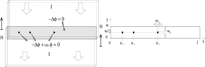
Figure 1: The left panel shows the top view of a superconducting microstrip line containing three Josephson junctions, $H,I$ and $\phi$ are respectively the applied magnetic field, current and the phase difference between the two superconducting layers. The phase difference $\phi$ between the two superconducting layers satisfies $-\Delta\phi=0$ in the linear part and $-\Delta\phi+\sin(\phi)=0$ in the Josephson junctions. The right panel shows the associated 2D domain of size $l\times w$ containing $n=3$ junctions placed at the positions $y=w/2$ and $x=a_{i},~{}i=1,n$.

The boundary conditions representing an external current input $I$ or an applied magnetic field $H$ (along the y axis) are

$$\left.\frac{\partial\varphi}{\partial y}\right|_{y=0}=-\frac{I}{2l}\nu,~{}\left.\frac{\partial\varphi}{\partial y}\right|_{y=w}=\frac{I}{2l}\nu,~{}\left.\frac{\partial\varphi}{\partial x}\right|_{x=0}=H-\frac{I}{2w}(1-\nu),~{}\left.\frac{\partial\varphi}{\partial x}\right|_{x=l}=H+\frac{I}{2w}(1-\nu)$$ (3)

where $0\leq\nu\leq 1$ gives the type of current feed. The case $\nu=1$ shown in Fig. 1 where the current is only applied to the long boundaries $y=0,w$ is called overlap feed while $\nu=0$ corresponds to the inline feed.

We consider long and narrow strips containing a few small junctions of area $w_{i}^{2}$ placed on the line $y=w/2$ and centered on $x=a_{i},~{}~{}i=1,n$ as shown in Fig. 1. Then we search $\varphi$ in the form

$$\varphi(x;y)=\frac{\nu I}{2L}\left(y-\frac{\omega}{2}\right)^{2}+\sum_{n=0}^{+\infty}\phi_{n}(x)\cos\left(\frac{n\pi y}{w}\right),$$ (4)

where the first term takes care of the $y$ boundary condition. For narrow strips $w<\pi$, only the first transverse mode needs to be taken into account [6] because the curvature of $\varphi$ due to current remains small. Inserting (4) into (2) and projecting on the zero mode we obtain the following equation for $\phi_{0}$ where the index $0$ has been dropped for simplicity

$$-\phi^{\prime\prime}+g\left(x,{w\over 2}\right){w_{i}\over w}\sin\phi=\nu\frac{\gamma}{l},$$ (5)

and where $\gamma=I/w$ and the boundary conditions $\phi^{\prime}(0)=H-(1-\nu)\gamma/2$, and $\phi^{\prime}(l)=H+(1-\nu)\gamma/2$. The factor $w_{i}/w$ is exactly the ”rescaling” of $\lambda_{J}(=1)$ into $\lambda_{eff}=\sqrt{w\over w_{j}}>1$ due to the presence of the lateral passive region [7].

As the area of the junction is reduced, the total Josephson current is reduced and tends to zero. To describe small junctions where the phase variation can be neglected but which can carry a significant current, we introduce the following function $g_{h}$

$$g_{h}(x)={w_{i}\over 2h},~{}~{}~{}{\rm for}~{}a_{i}-h<x<a_{i}+h,~{}~{}{\rm and}~{}~{}g_{h}(x)=0~{}~{}~{}~{}{\rm elsewhere},$$ (6)

where $i=1,..n$. In the limit $h\rightarrow 0$ we obtain our final delta function model [8]

$$-\phi^{\prime\prime}+\sum_{i=1}^{n}d_{i}\delta(x-a_{i})\sin\phi=\nu{\gamma\over l},$$ (7)

where $d_{i}=w_{i}^{2}/w$ and the boundary conditions are

$$\phi^{\prime}(0)=H-(1-\nu)\gamma/2,~{}~{}\phi^{\prime}(l)=H+(1-\nu)\gamma/2.$$

Despite its crude character the delta function approximation is a good model for arrays with short junctions as long as the magnetic field is small compared to $1/w_{i}$ where $w_{i}$ is the size of the junctions [10]. It allows simple calculations and in depth analysis that are out of reach for the 2D full model. In addition when $d_{i}<0$ the model can describe so-called $\pi$-junctions. For these, the tunneling current is $\sin(\phi+\pi)=-\sin(\phi)$ instead of the usual sine term in the second Josephson equation (1). This new type of coupling occurs in some materials [11, 12] and it is hoped to be incorporated in the design of arrays. It is then natural to associate negative $d_{i}$ coefficients to $\pi$ junctions in the device.

We have the following properties.

1. Integrating twice (7) shows that the solution $\phi$ is continuous at the junctions $x=a_{i},~{}i=1,\dots n$.

2. Almost everywhere (in the mathematical sense), $-\phi^{\prime\prime}(x)=\nu\gamma/l$, so that outside the junctions, $\phi$ is a piece-wise second degree polynomial,

   $$\phi(x)=-\frac{\nu\gamma}{2l}x^{2}+B_{i}x+C_{i}~{},~{}~{}\forall x\in]a_{i};a_{i+1}[.$$ (8)

3. At each junction ($x=a_{i}$), $\phi^{\prime}$ is not defined, but choosing $\epsilon_{1}>0$, and $\epsilon_{2}>0$, we note that

   $$\lim_{\epsilon_{1}\rightarrow 0}\lim_{\epsilon_{2}\rightarrow 0}\int_{a_{i}-\epsilon_{1}}^{a_{i}+\epsilon_{2}}\phi^{\prime\prime}(x)dx=\int_{a_{i}^{-}}^{a_{i}^{+}}\phi^{\prime\prime}(x)dx=\left[\phi^{\prime}(x)\right]_{a_{i}^{-}}^{a_{i}^{+}}.$$

   Since the phase is continuous at the junction $x=a_{i}$, $\phi_{i}\equiv\phi(a_{i})$ we get

   $$\left[\phi^{\prime}(x)\right]_{a_{i}^{-}}^{a_{i}^{+}}=d_{i}\sin(\phi_{i})\;.$$ (9)

4. Integrating (7) over the whole domain,

   $$\left[\phi^{\prime}\right]_{0}^{l}=\int_{0}^{l}\phi^{\prime\prime}dx=\sum_{i=1}^{n}d_{i}\sin(\phi_{i})-\nu\gamma~{},$$

   and taking into account the boundary conditions, we obtain

   $$\gamma=\sum_{i=1}^{n}d_{i}\sin(\phi_{i}),$$ (10)

   which indicates the conservation of current.

In [9], we developed two ways to find the $\gamma_{max}(H)$ curve for the device using these properties, see the Appendix ”Piece-wise polynomial” for more details on the solution of the problem. The most useful property in [9] for this study is the magnetic approximation of the $\gamma_{max}(H)$ curve.

3 The magnetic approximation

Since $\left[\phi^{\prime}\right]_{a_{i}^{-}}^{a_{i}^{+}}=d_{i}\sin(\phi_{i})$ (remark 9) and $\gamma\leq\sum_{i}d_{i}$, we notice that for small $d_{i}$, $\phi$ tends to the linear function $\phi(x)=Hx+c$. Starting from $\phi(x)\equiv Hx+c$, it is simple to find the $\gamma_{max}(H)$ curve. This is what we call the magnetic approximation. We generalize here what was done in [18] for arrays of equidistant junctions. We have shown in [9] that the $\gamma_{max}(H)$ curve of (7) tends to it when $d_{i}$ tends to zero. In experiments the $d_{i}$ coefficients are small enough so that this approximation is justified and provides a quantitative estimate of the $\gamma_{max}(H)$ curve [10]. For inhomogeneous arrays of many junctions, this curve is complex and even in this case the approximation is very good.

Since $\phi(x)=Hx+c$ then $\gamma=\sum_{i}d_{i}\sin(Ha_{i}+c)$. To find the $\gamma_{max}(H)$ curve of the magnetic approximation, we take the derivative of

$$\gamma=\left(\sum_{i=1}^{n}d_{i}\sin(Ha_{i})\right)\cos(c)+\left(\sum_{i=1}^{n}d_{i}\cos(Ha_{i})\right)\sin(c)\equiv A\cos(c)+B\sin(c),$$ (11)

with respect to $c$ where we have isolated the factors $A,B$. The values of $c$ such that $\partial\gamma/\partial c=0$ are

$$c_{max}(H)=\arctan\left(\frac{\sum_{i=1}^{n}d_{i}\cos(Ha_{i})}{\sum_{i=1}^{n}d_{i}\sin(Ha_{i})}\right)\;,$$ (12)

and as we want a maximal (not only an extremal) current we obtain:

$$\gamma_{max}(H)=\left|\sum_{i=1}^{n}d_{i}\sin\left(Ha_{i}+c_{max}(H)\right)\right|\;.$$ (13)

Now, we focus on the case where $c_{max}(H)$ is not defined. In this case, considering previous equation (12), we obtain $\sum_{i=1}^{n}d_{i}\sin(Ha_{i})=0=A$. From $A\sin(c)=B\cos(c)$ we obtain $\cos(c)=0$ or $B=0$. Note that $\cos(c)=0$ imply $\gamma=0$, in the other hand, $B=0$, imply $\partial\gamma/\partial c=0$ whatever the value of $c$. So, $\gamma$ is constant, and $\gamma_{max}=A=0$.

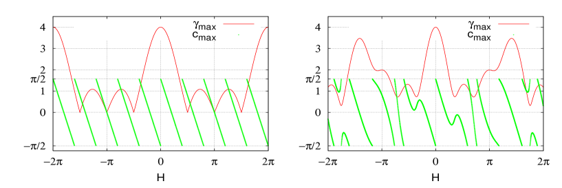
Figure 2: We plot $\gamma_{max}(H)$ and $c_{max}(H)$ for two four junction devices. In the left panel, we have a circuit with equidistant junctions of equal $d_{i}=1$. For the right panel, the junctions are such that $l_{1}=\frac{5}{2},~{}l_{2}=\frac{5}{3},~{}l_{3}=1$, with $d_{1}=1.2$, $d_{2}=1.5$, $d_{3}=0.5$, $d_{4}=0.8$. Notice that $c_{max}(H)$ varies in a complicated way for a non uniform device.

We plot $\gamma_{max}(H)$ and $c_{max}(H)$ in Fig.(2), for a uniform device and for a non uniform one. In the second case, we have chosen the position of the junction to have a long period ($H_{p}=12\pi$). We notice that the length $l$ of the device does not appear in eq. (13).

In order to study the function (13), we start with a few definitions.

$l_{i}$:

We define the distance between consecutive junctions:

$$l_{i}=a_{i+1}-a_{i}~{}.$$

Junction unit:

We call a junction unit the set of distances between junctions. We denote it

$$\{l_{1};l_{2};...;l_{n-1}\}~{}.$$

We define the position of the junction unit as $a_{1}$, the position of the first junction.

$l_{b}$:

For an $n$-junction device, $l_{b}=a_{n}-a_{1}$ is junction unit length.

Symmetric unit:

We call a symmetric unit, an $n$-junction circuit such that

$$\forall i\in\{1;\dots;n\},~{}~{}\frac{l_{b}}{2}-a_{i}=a_{n-i}-\frac{l_{b}}{2}\;,~{}~{}{\rm and}~{}~{}d_{i}=d_{n-i}\;.$$

In the Appendix we prove the following three Propositions

Invariance by translation

(7.1): $\gamma_{max}(H)$ does not depend on the position of the junction unit.

Parity of the $\gamma_{max}$ curve

(7.2): $\gamma_{max}(H)$ is an even function of $H$.

Solution for a symmetric device

(7.3): For a symmetric junction unit such that $a_{n}=-a_{1}$, $c_{max}(H)=\pm\pi/2$ (this is not obvious from fig.(2)).

In these propositions, we establish the most important result of this article. The $\gamma_{max}$ curve for a symmetric junction unit can be calculated simply by centering the junction unit so that $c_{max}(H)=\pm\pi/2$. More precisely, consider an $n+1$ symmetric junction unit where $n$ is even. We can always choose this by setting the $d$ of the central junction $(a_{1}+a_{n})/2$ to 0. Then we shift the junction unit by $a_{(n+1)/2}$ so that the central junction is placed at $x=0$. We relabel the junctions by setting $i^{\prime}=i-(n+1)/2$. Then the central one is for $i=0$, the first one to the right is $i=1$, the first one to the left is $i=-1$ …so that the equation (13) becomes

$$\gamma_{max}(H)=\left|d_{0}+2\sum_{i=1}^{(n+1)/2}d_{i}\cos(Ha_{i})\right|\;,$$ (14)

where we omitted the primes. In the rest of the article we will consider the array to be symmetric.

4 The direct problem for $\gamma_{max}$

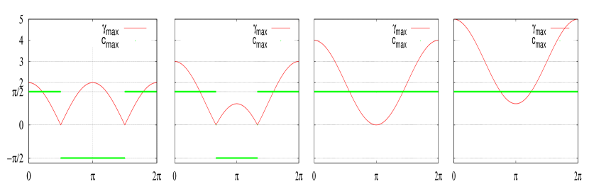
Figure 3: Curves $\gamma_{max}$ and $c_{max}$ versus $H$ for three junction devices, from left to right $d_{2}=0$, $d_{2}=1$, $d_{2}=2$ and $d_{2}=3$. For all panels, $a_{1}=-1$, $a_{2}=0$, $a_{3}=1$ and $d_{1}=d_{3}=1$.

4.1 A device such that $\gamma_{max}(H)=\cos(H)$

In Fig.(3) we present from left to right the $\gamma_{max}(H)$ for a SQUID (2 junctions), a uniform 3 junction unit, a $d_{1}=1=d_{3},~{}d_{2}=2$ (termed 1-2-1) junction unit that is discussed in [3] and a 1-3-1 junction unit. In all cases the junctions are equidistant. The first two panels, represent well known devices.

Applying eq.(14) to the following case $d_{2}=2$, we obtain,

$$\gamma_{max}(H)=|d_{0}+d_{1}\cos(Ha_{1})|=2+2\cos(Ha_{1})\;.$$ (15)

This is an exact cosine function shifted by a constant. With the last case $d_{2}=3$, we obtain $\gamma_{max}(H)=3+2\cos(Ha_{1})$.

Comparing all the panels we understand the role of the central junction. We can have an exact representation of $\gamma_{max}$ for this type of circuit, if we imagine $\gamma_{max}$ as an absolute value of a simple $\cos$ function translated by the value $d_{0}$ (which is equal to zero if there is no junction). Eq.(14) shows that we can sum cosine functions, with a chosen amplitude and period. Remark that if $d_{0}=-2$ ($\pi$ junction) then $\gamma_{max}(H)=2-2\cos(Ha_{1})$.

4.2 A multi-cosine $\gamma_{max}(H)$

For arrays with more than two junctions, experimentalists can play on the set of distances $l_{i}$ separating the junctions as well as on the strength $d_{i}$ (proportional to the area) of each junction. We now show the influence of each set of parameters starting from the $d_{i}$’s. Fig. 4 presents on the left panel $\gamma_{max}(H)$ for a symmetric set of 5 equidistant junctions $a_{1}=1,~{}a_{2}=2$. The dashed line corresponds to $d_{i}=1,~{}i=-2\dots 2$ giving a maximum current of 5. Here one sees the typical interference pattern between the main bumps. The small oscillations can be eliminated by choosing $d_{0}=1.82025,~{}d_{1}=d_{-1}=1.25$ and $d_{2}=d_{-2}=0.3425$ as seen from the continuous line on the left panel of Fig. 4. This ”pulse” profile could be very useful for specific applications because of the large region where $\gamma_{max}(H)=0$. The right panel of Fig. 4 presents what would be the device for this set of $a_{i}$ and $d_{i}$. We chose a critical current density of $10^{4}A~{}cm^{-1}$ so that $\lambda_{J}\approx 10\mu m$. We chose a transverse width $w=14\mu m$. Assuming the area of the smallest junction to be $1\mu m^{2}$, we get the scheme shown, where the central junction has an area 5.32 $\mu m^{2}$.

The second parameter that can be changed is the position $a_{i}$ of each junction in the array. As an example in Fig. 5 we show in the left panel the so-called ”triangle” $\gamma_{max}(H)$ obtained by setting $a_{1}=1,~{}a_{2}=3$, $d_{0}=2.4888,~{}d_{1}=1.1234$ and $d_{2}=0.121$. The dashed line presents $\gamma_{max}(H)$ for equal strengths. Changing the $d_{i}$’s allows to eliminate the oscillations in the minima of $\gamma_{max}(H)$ and obtain an almost linear behavior. The right panel shows the arrangement of the junctions in the microstrip. We have chosen the same physical parameters as for Fig. 4.

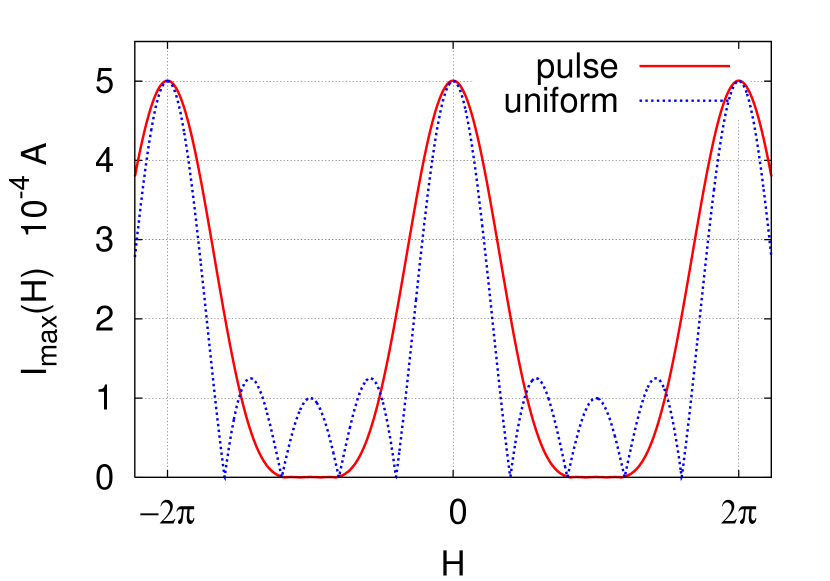
Figure 4: Left panel: plot of $\gamma_{max}(H)$ for a symmetric five equidistant junction device. The continuous line corresponds to different $d_{i}$ while the dashed line is for equal $d_{i}$. See the text for the parameter values. The right panel shows the corresponding device.

Now we can design all devices which have a $\gamma_{max}(H)$ curve as a sum of $d_{i}\cos(a_{i}x)$, with $d_{i}$ positive. We can notice that if $a_{i}/a_{1}\in\mathbb{R\backslash Q}$, we can construct a non periodic $\gamma_{max}(H)$.

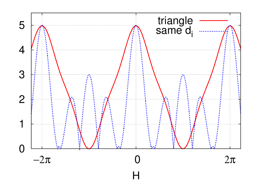
Figure 5: Left panel: plot of $\gamma_{max}(H)$ for a symmetric five junction device where the junctions are not equidistant, $a_{1}=1$ and $a_{2}=3$. The continuous line corresponds to different $d_{i}$ while the dashed line is for equal $d_{i}$. The right panel shows the corresponding device.

5 The inverse problem for a given $\gamma_{max}(H)=\gamma_{g}(H)$

We now show how to design an $n+1$ junctions circuit ($n$ is an even integer) to obtain a given $\gamma_{g}(H)$ curve. The formula (14) can be used to solve this inverse problem using cosine Fourier transforms. To avoid ambiguities we assume a symmetric array and a positive and periodic $\gamma(H)$.

We have the following result.

Proposition 5.1 (Solution of inverse problem for $\gamma_{max}(H)$)

Assume a $\gamma_{g}(H)$ even, periodic of period $H_{p}$ and strictly positive. The array is harmonic and the positions of the junctions are given by $a_{i}=i2\pi/H_{p}$ where $i$ is an integer. Their strengths $d_{i}$ are given by

$$d_{-i}=d_{i}=\frac{1}{H_{p}}\int_{0}^{H_{p}}\gamma_{g}(H)\cos(Ha_{i})dH~{},~{}~{}\forall i\in\{0,\dots,n/2\}~{}.$$ (16)

This gives the positions $a_{i}$ and coefficients $d_{i}$ of an array that will have a $\gamma_{max}(H)$ that is the truncation to order $n$ of the cosine Fourier series of $\gamma_{g}(H)$.

To gain insight into the problem let us first review the ”pulse” example studied in the previous section. Assume $\gamma_{g}(H)$ to be the $2\pi$ periodic extension of $e^{-\alpha H^{2}}$ where $\alpha$ is large enough. The coefficients $d_{i}$ are given by

$$d_{i}={1\over 2\pi}\int_{0}^{2\pi}e^{-\alpha H^{2}}\cos(Hi)~{}dH+{1\over 2\pi}\int_{0}^{2\pi}e^{-\alpha(2\pi-H)^{2}}\cos(Hi)~{}dH={1\over\pi}\int_{0}^{2\pi}e^{-\alpha H^{2}}\cos(Hi)~{}dH.$$ (17)

These Fourier coefficients decay exponentially as expected [17] because $\gamma_{g}(H)$ is $C^{\infty}$ over the interval $[0,2\pi]$ and satisfies the boundary conditions. This means that $i\leq 2$ is enough to get a good approximation of $\gamma_{g}(H)$. In fact Fig. 4 corresponds to $\gamma_{g}(H)\approx 5e^{-0.6H^{2}}$ and the formula (17) gives the values $d_{0}=1.82025,~{}d_{1}=d_{-1}=1.25$ and $d_{2}=d_{-2}=0.3425$ that were obtained in the previous section. The next coefficients $d_{3}=0.043$, $d_{4}=0.0023$ are very small and can be neglected.

Let us now consider a square $\gamma_{max}(H)$ curve which could make a very fine magnetic detector because of its strong response over a given interval and zero response elsewhere. For that we assume the the square profile

$$\gamma_{g}(H)=1~{}~{}{\rm for}~{}~{}\pi\left(1-{h_{1}\over 2}\right)<H<\pi\left(1-{h_{1}\over 2}\right)~{}~{}{\rm and}~{}~{}0~{}~{}{\rm elsewhere},$$ (18)

and extend it periodically every $2\pi=H_{p}$. To compute the parameters $a_{i}$ and $d_{i}$, we apply the previous result (see eq.(16)) to obtain

$$d_{i}={1\over 2\pi}\int_{0}^{2\pi}\gamma_{g}(H)\cos\left({i\pi H\over 2\pi}\right)dH={2\over i\pi}\sin\left(i\pi{h_{1}+h_{2}\over 2}\right)\cos\left({i\pi\over 2}+{h_{2}-h_{1}\over 2}\right)$$ (19)

This gives the following values of $d_{i}$ for $h_{1}=h_{2}=h$

$$\begin{array}[]{|c|c|c|c|c|c|c|}\hline\cr i&0&1&2&3&4&\dots\\ \hline\cr a_{i}&0&1&2&3&4&\dots\\ \hline\cr 2\pi d_{i}&2h&0&-{\sin(2\pi h)\over\pi}&0&{\sin(4\pi h)\over 2\pi}&\dots\\ \hline\cr\end{array}$$

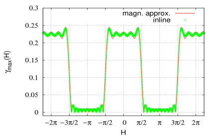
Figure 6: We compare the $\gamma_{max}(H)$ of the magnetic approximation to the exact solution of equation (7) for $\nu=0$ (inline current feed. The parameters are given in the text.

Note the decay in $1/i$ of $d_{i}$ because $\gamma_{g}(H)$ is only continuous. Another interesting fact is that some $d_{i}$ are negative so that some junctions are $\pi$ junctions. So we obtain an array of eleven junctions whose positions are given above together with their strengths $d_{i}$ (positive for a normal junction and negative for a $\pi$ junction).

In Fig. 6 we plot the magnetic approximation and the exact solution of equation (7) for $\nu=0$ (this case is called inline current feed, see the section ”Piece-wise polynomial” in the Appendix and for more details [9]). The values are $l=20$, the junction unit is shifted by $10$, the Josephson characteristic length is $\lambda_{J}=5.6\mu m$ so that all $d_{i}$ are multiplied by $0.035714285$.

We see that for this type of junction (about $1\mu m^{2}$ of area) inline current feed for (7) and magnetic approximation give close results. Differences appear when the maximal current is larger but the Gibbs phenomena is less important in the solution of the equation (7) than magnetic approximation.

6 Conclusion

Using a simple approximation, we introduced a method to design a symmetric array of Josephson junctions which has a specific $\gamma_{max}(H)$ static response. The sizes of the junctions are given by the coefficients $d_{i}$ of the cosine Fourier transform of $\gamma_{max}(H)$. Their position is $a_{i}=i2\pi/H_{p}$ where $H_{p}$ is the period of $\gamma_{max}(H)$. We use $2n+1$ junctions to obtain a curve formed with $n$ Fourier coefficients.

This work follows closely the article [9], where all the mathematical results were established, in particular the convergence of the solutions of the full problem (7) to the ones obtained in the magnetic approximation. There we show that the overlap current feed can cause a non even $\gamma_{max}(H)$ (see proposition ”Magnetic shift” in [9]).

If we are in the region of validity of our original model, ie the magnetic field is small and the distance between junctions is larger than their size, then we can design a device for a given static response.

Acknowledgements

The authors thank Faouzi Boussaha and Morvan Salez for useful discussions. L. L. thanks Delphine and Damien Belmessieri for their comments.

7 Appendix

7.1 Propositions

Proposition 7.1 (Invariance by translation)

The $\gamma_{max}(H)$ curve obtained within the magnetic approximation does not depend on the position of the junction unit.

Proof. Let us assume two devices with the same junction unit $\{l_{1};l_{2};...;l_{n}\}$ with the first junction placed respectively at $x=a_{1}$ and $x=a_{1}+c$. We note $\gamma^{1}_{max}(H)$ (respectively $\gamma^{2}_{max}(H)$) the $\gamma_{max}(H)$ curve of the first (respectively the second) device. In the same way we note $c_{max}^{1}(H)$ (respectively $c_{max}^{2}(H)$) the $c_{max}(H)$ function of the first (respectively the second) device.

$$\gamma^{2}_{max}(H)=\left|\sum_{i=1}^{n}d_{i}\sin\left(Ha_{i}+Hc+c_{max}^{2}(H)\right)\right|\;,$$

we note $c^{1}(H)=Hc+c_{max}^{2}(H)$. As we do not know if $c^{1}(H)=c_{max}^{1}(H)$, $c_{max}^{1}(H)$ being the best value (if it exists) to obtain the maximal $\gamma$. Consequently, $\gamma^{2}_{max}(H)\leq\gamma^{1}_{max}(H)$.

On the other side, considering

$$\gamma^{1}_{max}(H)=\left|\sum_{i=1}^{n}d_{i}\sin\left(H(a_{i}+c)+c_{max}^{1}(H)-Hc\right)\right|\;,$$

noting $c^{2}(H)=c_{max}^{1}(H)-Hc$ and using the previous argument, we obtain $\gamma^{2}_{max}(H)\geq\gamma^{1}_{max}(H)$. From the two previous inequalities, we obtain: $\gamma^{1}_{max}(H)=\gamma^{2}_{max}(H)$.      

Thus, the $\gamma_{max}(H)$ curve for the magnetic approximation depends only on the junction unit.

Proposition 7.2 (Parity of the $\gamma_{max}$ curve)

For all devices, $\gamma_{max}(H)=\gamma_{max}(-H)$.

Proof. Since $\sin$ and $\arctan$ are odd functions and $\cos$ is an even function then $c_{max}(-H)=-c_{max}(H)$ (see (12)). Finally,

$$\gamma_{max}(-H)=\left|\sum_{i=1}^{n}d_{i}\sin\left(-Ha_{i}-c_{max}(H)\right)\right|=\gamma_{max}(H)\;.$$

     

Notice that $c_{max}$ is an odd function and $\gamma_{max}$ is an even function (see Fig.(2) ).

Proposition 7.3 (Particular solution for symmetric device)

For all symmetric units such that $a_{n}=-a_{1}$, $c_{max}(H)=\pm\pi/2$.

Proof. To see this, relabel the junctions so that the central one corresponds to $i=0$, the 1st on the left to $i=-1$, the 1st on the right to $i=+1$.. Using the first proposition we can shift the junction unit so that $a_{0}=0$. Then the total current is

$$\gamma(H) = \sum_{i=-n/2}^{n/2}d_{i}\sin(Ha_{i}+c)$$

$$= d_{0}\sin(c)+2\sum_{i=1}^{n/2}d_{i}\sin(Ha_{i}+c)$$

$$= \sin(c)\left(d_{0}+2\sum_{i=1}^{n/2}d_{i}\cos(Ha_{i})\right)$$

Then $c_{max}=\pi/2$ when $d_{0}+2\sum_{i=1}^{n/2}d_{i}\cos(Ha_{i})\geq 0$ and $c_{max}=-\pi/2$ otherwise. Thus,

$$\gamma_{max}(H)=\left|d_{0}+2\sum_{i=1}^{(n+1)/2}d_{i}\cos(Ha_{i})\right|\;.$$ (20)

     

7.2 Piece-wise polynomial

Let $\phi$ be a solution of (7) and $\phi_{1}=\phi(a_{1})$. From remark (8), $\phi$ is a polynomial by parts. We define $P_{i+1}(x)$ the second degree polynomial such that $P_{i+1}(x)=\phi(x)~{}~{}{\rm for}~{}~{}a_{i}\leq x\leq a_{i+1}$. Using the left boundary condition we can specify $\phi$ on $[0;a_{1}]$:

$$P_{1}(x)=-\frac{\nu\gamma}{2l}\left(x^{2}-a_{1}^{2}\right)+\left(H-\frac{1-\nu}{2}\gamma\right)(x-a_{1})+\phi_{1}$$ (21)

At the junctions (9) tells us that $\forall k\in\{1;\dots;n\}$,

$$P_{k+1}^{\prime}(a_{k})-P_{k}^{\prime}(a_{k})=d_{k}\sin(P_{k}(a_{k})).$$ (22)

Considering that $\phi^{\prime\prime}=-\nu\gamma/l$ on each interval, the previous relation and the continuity of the phase at the junction, we can give a first expression for $P_{k+1}$,

$$P_{k+1}(x)=-\frac{\nu\gamma}{2l}(x-a_{k})^{2}+\left[P^{\prime}_{k}(a_{k})+d_{k}\sin P_{k}(a_{k})\right](x-a_{k})+P_{k}(a_{k}).$$ (23)

So, $\phi$ is entirely determined by $\phi_{1}$, $\gamma$ and $H$.

The polynomials (21) and (23) establish existence and shape of $\phi$ at junctions. Let see boundary conditions. The first,

$$\phi^{\prime}(0)=P_{1}^{\prime}(0)=H-(1-\nu)\gamma/2$$

is true by construction; the second (for $n$ junction circuit) is:

$$P^{\prime}_{n+1}(l)=H+(1-\nu)\frac{\gamma}{2},$$ (24)

is true only for solutions of Eq.(7). At $H$ given, solutions of Eq.(24) define a relation between $\phi_{1}$ and $\gamma$.

So, the maximal current solution depend on $\phi_{1}$ and $\gamma$, and Eq.(24) is the constraint for search of $\gamma_{max}(H)$. As solutions $\phi$ are defined at $2\pi$ almost (see equation (7)), we can assume $\phi_{1}\in[-\pi;\pi]$. In other hand, Rem.(10) teach us that $\gamma_{max}\in[0;\sum_{i}d_{i}]$, so we take $\gamma\in\left[0;\sum_{i}d_{i}\right]$. To solve this problem with Maple ©, we plot implicit function (the constraint) of two variables $\phi_{1}$ and $\gamma$, with $H$ and $\nu$ fixed. Let us note all variables:

$$\left.P^{\prime}_{n+1}\right|_{x=l}(\phi_{1},\gamma,\nu,H)-H-\frac{1-\nu}{2}\gamma=0.$$ (25)

with $(\phi_{1},\gamma)\in[-\pi;\pi]\times\left[0;\sum_{i}d_{i}\right]$. Lastly the program search in exhaustive way, the biggest value of $\gamma$ of this implicit curve. Incrementing $H$, we obtain $\gamma_{max}(H)$.

This method has the advantage to converge to the global maximal $\gamma_{max}$ [9].

References

- [1] B. D. Josephson, Possible new effects in supercondutive tunneling, Phys. Lett. 1, 251-253, (1962).
- [2] A. Barone and G. Paterno, Physics and Applications of the Josephson effect, J. Wiley, (1982).
- [3] K. Likharev, Dynamics of Josephson junctions and circuits, Gordon and Breach, (1986).
- [4] J. G. Caputo, N. Flytzanis and M. Vavalis, A semi-linear elliptic pde model for the static solution of Josephson junctions, International Journal of Modern Physics C, vol. 6, No. 2, 241-262, (1995).
- [5] M. H. Chung and M. Salez, Proc. 4th European Conference on applied superconductivity, EUCAS 99, 651, (1999).
- [6] J. G. Caputo, N. Flytzanis, Y. Gaididei and M. Vavalis, Two-dimensional effects in Josephson junctions: I static properties, Phys. Rev. E, 54, No. 2, 2092-2101, (1996).
- [7] J. G. Caputo, N. Flytzanis and M. Vavalis, Effect of geometry on fluxon width in a Josephson junction, Journal of Modern Physics C, vol. 7, No. 2, 191-216, (1996).
- [8] J. G. Caputo and L. Loukitch, Dynamics of point Josephson junctions in microstrip line., Physica 425 (2005) 69-89.
-
[9]
J. G. Caputo and L. Loukitch, Statics of
point Josephson junctions in a micro strip line., SIAM J. Appl. Math.
in press.
http://arxiv.org/abs/math-ph/0607018 -
[10]
F. Boussaha, J. G. Caputo, L. Loukitch and M. Salez,
SQUID properties of non-uniform, parallel
superconducting junction arrays.,
http://arxiv.org/abs/cond-mat/0609757. - [11] J. R. Kirtley et al, Science 90, 1373, (1999).
- [12] V. V. Razianov et al, Phys. Rev. Lett. 86, 2427, (2001).
- [13] J. G. Caputo and Y. Gaididei, Two point Josephson junctions in a superconducting stripline: static case., Physica C, 402, 160-173, (2004).
- [14] M. A. Itzler and M. Tinkham, Flux pinning in large Josephson junctions with columnar defects, Phys. Rev. B 51, 435, (1995).
- [15] M. A. Itzler and M. Tinkham, Vortex pinning by disordered columnar defects in large Josephson junctions, Phys. Rev. B 53, 11949, (1996).
- [16] R. Fehrenbacher, V. B. Geshkenbein and G. Blatter, Pinning phenomena and critical currents in disordered long Josephson junctions, Phys. Rev. B 45, 5450, (1992).
- [17] H. S. Carslaw, An introduction to the theory of Fourier series and integrals, Dover, (1950).
- [18] J. H. Miller, Jr., G. H. Gunaratne, J. Huang, and T. D. Golding, Enhanced quantum interference effects in parallel Josephson junction arrays, Appl. Phys. Lett. 59, (25), 3330 (1991).