Efficient calculation of van der Waals dispersion coefficients with time-dependent density functional theory in real time: application to polycyclic aromatic hydrocarbons

Abstract

The van der Waals dispersion coefficients of a set of polycyclic aromatic hydrocarbons, ranging in size from the single-cycle benzene to circumovalene (C₆₆H₂₀), are calculated with a real-time propagation approach to time-dependent density functional theory (TDDFT). In the non-retarded regime, the Casimir-Polder integral is employed to obtain $C_{6}$, once the dynamic polarizabilities have been computed at imaginary frequencies with TDDFT. On the other hand, the numerical coefficient that characterizes the fully retarded regime is obtained from the static polarizabilities. This ab initio strategy has favorable scaling with the size of the system – as demonstrated by the size of the reported molecules – and can be easily extended to obtain higher order van der Waals coefficients.

I INTRODUCTION

When two molecules are far apart, they still interact through long range electromagnetic forces, named after J. D. van der Waals.vanderWaals-1869 These are crucial to understand a wide range of phenomena: the chemistry of rare gases,christe-2001 protein folding and dynamics,roth-1996 the machinery of neurotransmitterssiegel-2006 and the molecular chemistry in the interstellar mediumnaray-szabo-1990 are just some examples. In particular, in astrochemistry van der Waals forces are essential to describe neutral-neutral reactions, which are not yet well accounted for in rate-reaction models. These intermolecular forces are mainly originated by electric multipole-multipole interactions. Even if the static multipoles of the molecules are null (as the dipole of a single spherical atom in the ground state), they still contribute to the interaction due to their spontaneous oscillations. These contributions of dynamical origin, that cannot be explained by Electrostatics, are the London dispersion forces.london-1936 These are attractive interactions, and arise from the mutual polarization of the two electronic clouds. They dominate the long range dynamics of the molecules, and are also present at short distances – although masked by other stronger (ionic or covalent) forces.

The calculation of these dispersion forces can be a challenging problem.dobson-2001 Three regimes have to be distinguished, according to the distance that separates the interacting molecules:

(i) short distances, such that there is non-negligible overlap of the electronic clouds of the two molecules. This is the most difficult situation, since it requires, in principle, a supermolecule calculation, i.e. the treatment of the two molecules combined together as a single entity. The valid approaches in this overlapping regime (and therefore also valid in the non-overlapping regime) are sometimes called seamless van der Waals techniques. Numerous possibilities exist, although none of them entirely satisfactory: full configuration interaction for very small molecules,lee-2001 Møller-Plesset perturbation theoryrowley-2006 or Monte Carlo methods.anderson-1993 Attempts to use ground state density functional theory (DFT) are specially challenging;dobson-2001 In the realm of time-dependent density-functional theory (TDDFT), the recent work of Dobson dobson-2006 summarizes the current research, largely based on the adiabatic connection / fluctuation dissipation theorem. Dispersive forces can also be added to standard DFT through empirical correction terms. These, however, require the previous knowledge of the $C_{6}$ van der Waals coefficients (see below), often roughly estimated from the atomic $C_{6}$’s .grimme-2004-2005 In the present work we will not consider this regime.

(ii) long distances, such that we can neglect the overlap. In this case, the electrons belonging to different molecules are distinguishable, and one can isolate the Coulomb operator that corresponds to interactions between electrons of different molecules, and apply (second order) perturbation theory for this operator.jeziorsky-1994 The first term in the perturbative expansion of the interaction energy decays as $-C_{6}/R^{6}$, where $R$ is the intermolecular distance.

(iii) very long distances, such that retardation effects become important.casimir-1948 This means that the time it takes for the photons that mediate the electromagnetic interaction to travel between the two molecules is not negligible. Retardation is described by a correction factor that is equal to unit for small distances and proportional to $1/R$ for large distances.

The knowledge of the various static and dynamic multipole polarizabilities at imaginary frequencies suffices to compute the van der Waals interaction in the regimes (ii) and (iii). These response functions can be calculated within a variety of quantum chemical methods, typically through the evaluation of a wide range of excitation energies and associated transition matrix elements. Alternatively, at a lower computational cost, we can use time-dependent density-functional theory (TDDFT).runge-1984 ; tddft-book This theory is very successful in predicting optical spectra (i.e., essentially the imaginary part of the dynamic polarizability at real frequencies) for finite systems, and has been used to study a wealth of molecules and clusters.castro-2004 The first calculation of $C_{6}$ coefficients using TDDFT was performed in 1995 by van Gisbergen et al for a variety of small molecules.vanGisbergen-1995

TDDFT in the perturbative regime can be formulated in a variety of flavors.marques-2006 With the purpose of calculating $C_{6}$ coefficients, one can find several approaches. Van Gisbergen et alvanGisbergen-1995 opted for a self-consistent calculation of the response function. The matrix formulation of linear response theorycasida-1995 can also be employed, yielding oscillator strengths and excitation energies, sufficient ingredients for the computation of the dynamic polarizability. A slightly different approach is the polarization propagator technique,oddershede-1984 which can be constructed on top of TDDFT (or on top of other electronic structure theories, e.g. time-dependent Hartree-Fock, TDHF). The linear polarization propagator was demonstrated to work for complex frequenciesnorman-2001 , opening the possibility of computing $C_{6}$ coefficients.norman-2003 With this technique, Jiemchooroj and collaborators computed $C_{6}$ coefficients of noble gases atoms,norman-2003 $n$-alkanesnorman-2003 ($n\leq 7$), polyacenes,jiemchooroj-2005 the C₆₀ molecule,jiemchooroj-2005 and sodium clusters up to 20 atomsjiemchooroj-2006 . For large molecules, Banerjee and Harbola have proposed the use of orbital free TDDFT,banerjee-2002 providing satisfactory results for large sodium clusters.

In this work, we propose an alternative scheme, based on the explicit propagation of the time-dependent Kohn-Sham equations.yabana-1996 ; yabana-1999 This approach has already proved its usefulness to calculate the dynamic polarizability of large systems (see, e.g., Ref. lopez-2005, ). The explicit time-dependent picture, where one is confronted with an initial value problem, can be preferable over the the time-independent picture – where the mathematical problem is diagonalization –, especially regarding scalability with the size of the system. For a discussion in the field of TDDFT, see Ref. marques-2006, .

We have chosen an extensive set of polycyclic aromatic hydrocarbons (PAHs) in order to validate the methodology. PAHs, a large class of conjugated $\pi$-electron systems, are of great importance in many areas, among which combustion and environmental chemistry, materials science, and astrochemistry. PAHs are found in carbonaceous meteorites, in interplanetary dust particles, and are thought to be the most abundant molecular species in space after H2 and CO, playing a crucial role in the energy and ionization balance of interstellar matter in galaxies. Motivated by this astrochemical relevance, some of us have recently performed an extensive study of these systems.malloci-2004 ; malloci-2007-II This research is collected in a thorough compendium of molecular properties of PAHs.malloci-2007-II The computation of van der Waals constants for pairs of PAHs, as a first approach to the analysis of their intermolecular properties, is therefore a natural extension of this work. In fact, van der Waals parameters are a crucial ingredient to model condensation and evaporation of PAH clusters, which are another important player in the physics/chemistry of the interstellar medium. In current works, people usually employ empirical van der Waals parameters for the relatively long-range part of the interaction in molecular dynamics simulations, together with some tight-binding approximation for the short-range part. rapacioli-2005-2006

One previous calculation of dispersion coefficients of PAHs, based on the complex linear polarization propagator method, was reported in Ref. jiemchooroj-2005, , although limited to benzene, naphthalene, anthracene, and naphtacene. This fact adds a further motivation to our study, since it permits to compare the results of the two schemes.

II METHODOLOGY

When both the wavefunction overlap and the retardation effects are almost null [situation (ii)], the application of second order perturbation theory leads to an expansion of the interaction energy with respect to the inverse of the intermolecular distance $(1/R)$:

$$\Delta E(R)=-\sum_{n=6}^{\infty}\frac{C_{n}}{R^{n}}\,.$$ (1)

The coefficients $C_{n}$ are usually called Hamaker constants.hamaker-1937 The leading non-null term $C_{6}$ is due to the dynamic dipole-dipole polarizability. The odd terms until $n=11$ are also null for spherical molecules (or if an average over relative orientations is taken), if we neglect retardation effects. In principle, the coefficients also depend on the relative orientation of the molecules.

The $C^{AB}_{6}$ dispersion Hamaker constant for a pair of molecules $A$ and $B$, averaged over all possible relative orientations, is related to the dipole molecular polarizability through the Casimir-Polder relation (atomic units will be used hereafter):

$$C^{AB}_{6}=\frac{3}{\pi}\int_{0}^{\infty}\!\!\!{\rm d}u\;\alpha^{(A)}({\rm i}u)\;\alpha^{(B)}({\rm i}u)\,,$$ (2)

where $\alpha^{(X)}({\rm i}u)$ is the average of the dipole polarizability tensor of molecule $X$, $\bm{\alpha}^{(X)}$, evaluated at the complex frequency ${\rm i}u$:

$$\alpha^{(X)}({\rm i}u)=\frac{1}{3}{\rm Tr}[\bm{\alpha}^{(X)}({\rm i}u)]\,.$$ (3)

It should be noted that: (i) If we fix the relative orientation of the molecules, the orientation dependent Hamaker constant can also be calculated from the $\bm{\alpha}$ tensors, considering the appropriate linear combination of their components; (ii) higher order Hamaker constants, useful for shorter distances, can be obtained through the use of analogous formulae involving higher order multipole polarizability tensors. The expressions accounting for these two generalizations can be found, for example, in Ref. jeziorsky-1994, . The calculations presented below are solely concerned with Eq. (2); however we wish to stress that the methodology trivially yields full polarizability tensors of arbitrary order, hence providing the possibility to tackle those general cases, with almost no extra computational cost.

On the other hand, when the distance increases and retardation effects become important, the van der Waals interaction depends solely on the static polarizability,casimir-1948 ; calbi-2003 decaying as $\Delta E(R)=-K^{AB}/R^{7}$, where the constant is

$$K^{AB}=\frac{23c}{8\pi^{2}}\alpha^{(A)}(0)\;\alpha^{(B)}(0)\,,$$ (4)

where $c$ is the velocity of light in vacuum.

The TDDFT time propagation approach to obtain the dynamic polarizability components can be summarized as follows: let us assume a weak electrical (spin-independent) dipole perturbation

$$\delta v_{{\rm ext},\sigma}({\bf r},\omega)=-x_{j}\kappa(\omega)\,.$$ (5)

This defines an electrical perturbation polarized in the direction $j$: $\delta{\bf E}(\omega)=\kappa(\omega)\hat{e}_{j}$. The response of the system dipole moment in the $i$ direction

$$\delta\langle\hat{X}_{i}\rangle(\omega)=\sum_{\sigma}\int\!\mathrm{d}^{3}r\,x_{i}\;\delta n_{\sigma}({\bf r},\omega)$$ (6)

is then given by:

$$\delta\langle\hat{X}_{i}\rangle(\omega)=-\kappa(\omega)\sum_{\sigma\sigma^{\prime}}\int\!\mathrm{d}^{3}r\,\!\!\int\!\mathrm{d}^{3}r^{\prime}\,x_{i}\;\chi_{\sigma\sigma^{\prime}}({\bf r},{\bf r}^{\prime},\omega)\;x^{\prime}_{j}\,,$$ (7)

where $\chi_{\sigma\sigma^{\prime}}$ is the response function of the system:

$$\delta n_{\sigma}({\bf r},\omega)=\sum_{\sigma\sigma^{\prime}}\int\!\mathrm{d}^{3}r\,\chi_{\sigma\sigma^{\prime}}({\bf r},{\bf r}^{\prime},\omega)\delta v_{{\rm ext},\sigma^{\prime}}({\bf r}^{\prime},\omega)\,.$$ (8)

The dynamic dipole polarizability $\alpha_{ij}(\omega)$ is the quotient of the induced dipole moment in the direction $i$ with the applied external electrical field in the direction $j$, which yields:

$$\alpha_{ij}(\omega)=-\sum_{\sigma\sigma^{\prime}}\int\!\mathrm{d}^{3}r\,\!\!\int\!\mathrm{d}^{3}r^{\prime}\,x_{i}\;\chi_{\sigma\sigma^{\prime}}({\bf r},{\bf r}^{\prime},\omega)\;x^{\prime}_{j}\,.$$ (9)

The dynamic polarizability elements may then be arranged to form a second-rank symmetric tensor, $\bm{\alpha}(\omega)$. We consider now a sudden external perturbation at $t=0$ (delta function in time, which means $\kappa(\omega)=\kappa$, equal for all frequencies), applied along a given polarization direction, say $\hat{e}_{j}$. By propagating the time-dependent Kohn-Sham equations,castro-2004-II we obtain $\delta n({\bf r},t)$. The polarizability element $\alpha_{ij}(\omega)$ may then be calculated easily via:

$$\alpha_{ij}(\omega) = -\frac{\delta\langle\hat{X}_{i}\rangle(\omega)}{\kappa}=-\frac{1}{\kappa}\int\!\mathrm{d}^{3}r\,x_{i}\;\delta n({\bf r},\omega)=$$ (10)

$$-\frac{1}{\kappa}\int\!\!{\rm d}t\int\!\mathrm{d}^{3}r\,x_{i}\;\delta n({\bf r},t)e^{-\mathrm{i}\omega t}$$

In order to obtain values of $\alpha$ at imaginary frequencies one only has to substitute $\omega$ by ${\rm i}u$. This computational framework has been implemented in the octopus code, described in Ref. octopus-1, , to which we refer the reader for technical details. The octopus code performs the calculation on a real space mesh, which reduces the convergence problem to two parameters: the grid spacing (we used 0.3 Å  in this case) and the size of the simulation box. The ion-electron interaction was modelled with norm-conserving Troullier-Martins pseudopotentials.troullier-1991

The geometries of the PAHs were obtained by means of DFT as described in Ref. malloci-2007-II, . For the optimization of the geometries, we chose the hybrid B3LYPbecke-1993 as the approximation to the exchange and correlation functional. For the TDDFT propagations, however, we used the adiabatic local density approximation (LDA), which has proved to yield reliable results for conjugated molecules;yabana-1999 the use of more sophisticated functionals is possible, but does not change the results for the dynamic polarizability significantly.marques-2001

III RESULTS

We have computed the $C^{AB}_{6}$ Hamaker constants for all possible pairs $\{A,B\}$ of a set of 41 PAHs. The homo-molecular Hamaker constants $C^{AA}_{6}$ for all the PAHs studied are reported in Tables 1 and 2; the full set can be consulted in the database described in Ref. malloci-2007-II, . The tables also display the average static dipole polarizability $\alpha(0)$, the effective London frequency $\omega_{1}$ (see below) and the retarded van der Walls coefficient $K$.

It is very difficult to extract Hamaker constants experimentally; to our knowledge, there are no experimental results reported for any PAH to compare to. For benzene, however, Kumar and Meithkumar-1992 reported a value of 1723 a.u., by making use of the dipole oscillator strength distributions (DOSDs), which are constructed from experimental dipole oscillator strengths and molar refractivity data. This is in good agreement with our computed value of 1763 a.u.

We have also displayed for comparison the numbers reported in Ref. jiemchooroj-2005, , obtained by means of the complex linear polarization propagator scheme. This scheme was constructed on top of TDDFT, although making use of the B3LYP functional. These methodological differences, and further numerical details can explain the very small differences, in all cases below 2% – see the results in the Table 1 for benzene, naphthalene, anthracene and tetracene (also known as naphthacene).

In the so-called London approximation, the polarizability at imaginary frequencies is modelled with the help of only two parameters: the static polarizability, and one effective frequency $\omega_{1}$:

$$\alpha({\rm i}u)=\frac{\alpha(0)}{1+(u/\omega_{1})^{2}}\,.$$ (11)

Upon substitution on the Casimir-Polder integral, this yields for a homo-molecular Hamaker constant:

$$C_{6}=\frac{3\omega_{1}}{4}\alpha^{2}(0)\,.$$ (12)

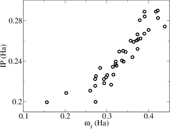
Figure 1: Ionization potentials (vertical axis) against dispersion frequencies (horizontal axis) for all the PAHs under study

With the knowledge of $C_{6}$ and $\alpha(0)$, one can obtain $\omega_{1}$ from Eq. 12. These effective frequencies are also reported in Tables 1 and 2. They are roughly decreasing with the size of the PAH, from 0.482 Ha for benzene to the 0.156 Ha of pentarylene. The decrease is, however, strongly irregular. As it has been pointed out beforemahan-1990 , it can be related to the ionization potential of the molecules; this is demonstrated in Fig. 1, where we have plotted the ionization potentials of the PAHs (calculated at the DFT/B3LYP level of theory), versus the effective frequency $\omega_{1}$. The data points approximately accumulate around a straight line, proving the correlation.

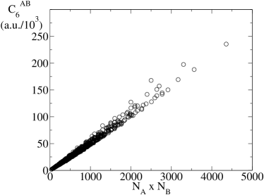
Figure 2: $C_{6}^{AB}$ Hamaker constants for all the pairs of PAHs under study, as a function of the product of the number of Carbon atoms, $N_{A}\times N_{B}$.

Equation 12 also gives us a hint on the dependency of $C_{6}$ with the size of the molecule: it is proportional to the square of the polarizability (the product of polarizabilities, if the molecules are different), which in turn typically grows with the volume, and therefore, with the number of atoms. Consequently, one should expect a linear dependency of $C_{6}^{AB}$ with respect to the product of the number of atoms, $N_{A}\times N_{B}$. This is indeed confirmed in Fig. 2. Some cases, however, deviate from a straight line. These cases correspond to strongly anisotropic PAHs (with three very different axes). This is captured by the dipole anisotropy:

$$\Delta\alpha^{2}=\frac{1}{3}[(\alpha_{xx}-\alpha_{yy})^{2}+(\alpha_{xx}-\alpha_{zz})^{2}+(\alpha_{yy}-\alpha_{zz})^{2}]\,.$$ (13)

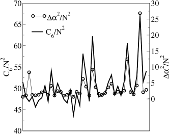
Figure 3: $C_{6}$ homo-molecular Hamaker constants divided by the square of the number of atoms (thick solid line, left axis), and dipole polarizability anisotropy, also divided by the square of the number of atoms (circles, right axis). Each data point corresponds with one PAH, ordered in the $x$-axis according to its number of atoms (it is the same ordering used in Tables 1 and 2).

Figure 3 shows how the PAHs whose Hamaker constant deviates strongly from the general trend are those whose polarizability anisotropy is also stronger: we have overlaid the values of $C_{6}$ for all PAHs (divided by the square of the number of Carbon atoms $N^{2}$), with the values $\Delta\alpha^{2}$ (also divided by $N^{2}$). One can see how the two datasets are correlated – specially in the right side of the graph, which corresponds to the larger PAHs.

The crossover between the non-retarded and retarded regimes is given by the length scale $\lambda=2\pi c/\bar{\omega}$, where $\bar{\omega}$ is a characteristic frequency of the electronic spectrum of the molecule. For $R/\lambda\gtrsim 10$ we enter the fully retarded regime, while for $R/\lambda\lesssim 0.1$ we can still use Eq. (1). Using for $\bar{\omega}$ the values of $\omega_{1}$ obtained through the London approximation, we reach values in the range of $\lambda\sim 0.1\,\mu$m (for benzene) to $\lambda\sim 0.3\,\mu$m (for pentarylene).

It is interesting to notice that in the fully retarded regime we can write $K^{AA}$ as a function solely of the Hamaker $C^{AA}_{6}$ coefficient and the effective London frequency $\omega_{1}$. Combining equations (4) and (12) we arrive at

$$K^{AA}=\frac{23c}{6\pi^{2}}\frac{C_{6}}{\omega_{1}}\,.$$ (14)

The values of homomolecular coefficients $K^{AA}$ for the PAHs studied in this work can be found in Tables 1 and 2.

IV CONCLUSIONS

In this Article we presented a method to calculate the van der Waals coefficients of molecular systems using a time-propagation scheme within TDDFT. As an example, we have applied this method to the family of polycyclic aromatic hydrocarbons. Our results are in excellent agreement with available theoretical and experimental data, and fully validate our approach. Values of $C_{6}$ scale approximately with $N_{A}\times N_{B}$, where $N_{X}$ is the number of atoms in the molecule $X$. The strongest deviations from this law are for highly anisotropic structures.

This scheme has several non-trivial advantages: (i) It scales with $N_{a}^{2}$, where $N_{a}$ is the number of atoms in the molecule. (ii) The time-propagation yields the polarizability in real time. From this quantity it is then immediate to obtain the real and imaginary parts of $\alpha$ at real and imaginary frequency. Therefore, the optical absorption spectrum, static polarizabilities, $C_{6}$ coefficients, etc. are calculated in one shot. (iii) This scheme is easily generalized to higher order coefficients and arbitrary geometries. We therefore expect it to be useful in the study of large systems, like clusters or molecules with biological interest.

Table 1: Average static polarizability $\alpha(0)$, $C_{6}$ Hamaker constant, effective frequency $\omega_{1}=(4/3)C_{6}/\alpha^{2}(0)$, and the coefficient $K$ of the retarded van der Waals interaction for the selected PAHs. All quantities are given in atomic units.

Molecule	$\alpha(0)$	$C_{6}$	$\omega_{1}$	$K$
		$\times 10^{-3}$		$\times 10^{-6}$
benzene (C6H6)	70.5	1.76	0.473	0.198
(Ref. jiemchooroj-2005, ; TDDFT/B3LYP)	70.0	1.77	0.482	0.195
(Ref. kumar-1992, ; DOSD)	67.8	1.72	-	-
azulene (C10H8)	133	5.15	0.390	0.703
naphthalene (C10H8)	123	4.79	0.422	0.605
(Ref. jiemchooroj-2005, ; TDDFT/B3LYP)	122	4.87	0.439	0.594
acenaphthene (C12H10)	143	6.76	0.439	0.820
biphenylene (C12H8)	152	6.91	0.400	0.920
acenaphthylene (C12H8)	145	6.57	0.417	0.838
fluorene margin (C13H10)	159	7.97	0.422	1.00
phenanthrene (C14H10)	182	9.36	0.379	1.32
anthracene (C14H10)	189	9.92	0.372	1.42
(Ref. jiemchooroj-2005, ; TDDFT/B3LYP)	185	10.0	0.392	1.37
pyrene (C16H10)	205	12.0	0.380	1.68
tetracene (C18H12)	264	17.5	0.336	2.78
(Ref. jiemchooroj-2005, ; TDDFT/B3LYP)	259	17.5	0.349	2.68
triphenylene (C18H12)	231	15.7	0.390	2.14
benzo[a]anthracene (C18H12)	246	16.6	0.364	2.42
chrysene (C18H12)	239	15.9	0.373	2.27
benzo[e]pyrene (C20H12)	260	18.9	0.375	2.69
perylene (C20H12)	262	18.6	0.361	2.74
benzo[a]pyrene (C20H12)	277	19.8	0.345	3.06
corannulene (C20H12)	244	17.5	0.390	2.38

Table 2: Continuation of Table 1.

Molecule	$\alpha(0)$	$C_{6}$	$\omega_{1}$	$K$
		$\times 10^{-3}$		$\times 10^{-6}$
anthanthrene (C22H12)	304	23.5	0.340	3.69
benzo[g,h,i]perylene (C22H12)	282	22.2	0.373	3.17
pentacene (C22H14)	353	28.1	0.301	4.98
dibenzo[b,def]chrysene (C24H14)	355	30.4	0.321	5.04
coronene (C24H12)	318	27.0	0.357	4.03
hexacene (C26H16)	454	42.1	0.272	8.23
dibenzo[cd,lm]perylene (C26H14)	384	34.8	0.314	5.89
bisanthene (C28H14)	402	37.6	0.310	6.45
benzo[a]coronene (C28H14)	386	37.9	0.339	5.96
dibenzo[bc,ef]coronene (C30H14)	431	44.0	0.316	7.42
dibenzo[bc,kl]coronene (C30H14)	459	46.3	0.293	8.40
terrylene (C30H16)	484	47.8	0.272	9.36
ovalene (C32H14)	453	49.6	0.323	8.18
tetrabenzocoronene (C36H16)	565	65.4	0.273	12.8
circumbiphenyl (C38H16)	538	69.8	0.321	11.6
circumanthracene (C40H16)	612	82.5	0.293	15.0
quaterrylene (C40H20)	799	97.0	0.203	25.5
circumpyrene (C42H16)	631	89.0	0.298	15.9
hexabenzocoronene (C42H18)	590	85.9	0.330	13.9
dicoronylene (C48H20)	770	122	0.274	23.6
pentarylene (C50H24)	1196	168	0.156	57.1
circumcoronene (C54H18)	840	150	0.284	28.1
circumovalene (C66H20)	1099	236	0.260	48.2

References

- (1) J. D. van der Waals, Over de Continuiteit van den Gas- en. Vloeistoftoestand, Ph. D. thesis, Univ. Leiden (1873); translated to English by R. Threlfall and J. F. Adair, Phys. Mem. 1, 333 (1890); J. S. Rowlinson, Nature 244, 414 (1973).
- (2) K. O. Christe, Angew. Chem. Int. Ed. 40, 1419 (2001).
- (3) C. M. Roth, B. L. Neal, and A. M. Lenhoff, Biophys. J. 70, 977 (1996).
- (4) G. J. Siegel, R. W. Albers, S. Brady and D. L. Price (Eds.), Basic Neurochemistry, Elsevier Academic Press, London (2006).
- (5) D. R. Flower (Ed.), Molecular Collisions in the interstellar medium, Astrophysics Series 17, Cambridge University Press, Cambridge (1990).
- (6) F. London, Trans. Far. Soc. 37, 8 (1936); J. Mahanty and B. W. Ninham, Dispersion Forces, Academic Press, London (1976); V. A. Parsegian, Van der Waals Forces: A Handbook for Biologists, Chemists, Engineers and Physicists, Cambridge University Press, New York (2006).
- (7) J. F. Dobson, K. McLennan, A. Rubio, J. Wang, T. Gould, H. M. Le and B. P. Dinte, Aust. J. Chem. 54, 513 (2001); A. D. Buckingham, P. W. Fowler and J. M. Hunter, Chem. Rev. 88, 963 (1988).
- (8) J. S. Lee, Chem. Phys. Lett. 339, 133 (2001); D. E. Woon, J. Chem. Phys. 100, 2838 (1994).
- (9) R. L. Rowley, C. M. Tracy, C. M. Pakkanen and T. A Pakkanen, J. Chem. Phys. 125, 154302 (2006).
- (10) J. B. Anderson, C. A. Traynor and B. M. Boghosian, J. Chem. Phys 99, 345 (1993); J. B. Anderson, J. Chem. Phys. 115, 4546 (2001).
- (11) J. F. Dobson, in Ref. tddft-book, , Chapter 30, p. 443.
- (12) See e.g. S. Grimme, J. Comput. Chem. 25, 1463 (2004); M. Piacenza and S. Grimme, J. Am. Chem. Soc. 127, 14841 (2005).
- (13) B. Jeziorski, R. Moszynski and K. Szalewicz, Chem. Rev. 94, 1887 (1994).
- (14) H. B. G. Casimir and D. Polder, Phys. Rev. 73, 360 (1948).
- (15) E. Runge and E. K. U. Gross, Phys. Rev. Lett. 52, 997 (1984); M.A.L. Marques, E.K.U. Gross, Annual Review of Physical Chemistry 55, 427 (2004); E. K. U. Gross, J. Dobson, and M. Petersilka, in Density Functional Theory II, edited by R. F. Nalewajski, Topics in Current Chemistry, Vol. 181, Springer, Berlin (1996), p. 81.
- (16) M. A. L. Marques, C. Ullrich, F. Nogueira, A. Rubio and E.K.U. Gross, editors, Time-Dependent Density-Functional Theory, Lecture Notes in Physics 706, Springer Verlag, Berlin (2006);
- (17) A. Castro, M. A. L. Marques, J. A. Alonso and A. Rubio, J. Comp. Theor. Nanoscience 1, 231 (2004).
- (18) S. J. A. van Gisbergen, J. G. Snijders and E. J. Baerends, J. Chem. Phys. 103, 9347 (1995).
- (19) M. A. L. Marques and A. Rubio, in Ref. tddft-book, , Chapter 15, p. 227.
- (20) M. E. Casida, in Recent Advances in Density Functional Methods, D. E. Chong (Ed.), Recent Advances in Computational Chemistry 1, World Scientific, Singapore (1995), pp. 155-192; M. E. Casida, in Recent Developments and Applications of Modern Density Functional Theory, J. M. Seminario (Ed.), Elsevier, Amsterdam (1996), pp. 391-439; M. E. Casida, C. Jamorski, K. C. Casida and D. R. Salahub, J. Chem. Phys. 108, 4439 (1998); M. Petersilka, E. K. U. Gross and K. Burke, Int. J. Quant. Chem. 80, 534 (2000).
- (21) J. Oddershede, P. Jørgensen and D. L. Yeager, Comput. Phys. Rep. 2, 33 (1984).
- (22) P. Norman, D. M. Bishop, H. J. A. Jensen and J. Oddershede, J. Chem. Phys. 115, 10323 (2001).
- (23) P. Norman, A. Jiemchooroj and B. E. Semelius, J. Chem. Phys. 118, 9167 (2003).
- (24) A. Jiemchooroj, P. Norman and B. E. Semelius, J. Chem. Phys. 123, 124312 (2005).
- (25) A. Jiemchooroj, P. Norman and B. E. Semelius, J. Chem. Phys. 125, 124306 (2006).
- (26) A. Banerjee and M. K. Harbola, J. Chem. Phys. 117, 7845 (2002); A. Banerjee and M. K. Harbola, PRAMANA J. Phys. 66, 423 (2006).
- (27) K. Yabana and G. F. Bertsch, Phys. Rev. B 54, 4484 (1996). K. Yabana and G. F. Bertsch, Z. Phys. D 42, 219 (1997).
- (28) K. Yabana and G. F. Bertsch, Int. J. Quantum Chem. 75, 55 (1999).
- (29) X. López, M.A.L. Marques, A. Castro and A. Rubio, J. Am. Chem. Soc. 127, 12329 (2005).
- (30) G. Malloci, G. Mulas and C. Joblin, Astron. Astrophys. 426, 105 (2004). G. Malloci, G. Mulas, G. Cappellini, V. Fiorentini and I. Porceddu, Astron. Astrophys. 432, 585 (2005). G. Malloci, C. Joblin and G. Mulas, Astron. Astrophys. 462, 627 (2007).
- (31) G. Malloci, C. Joblin and G. Mulas, Chem. Phys. 332, 353 (2007); http://astrochemistry.ca.astro.it/database/
- (32) See e.g. M. Rapacioli, F. Calvo, F. Spiegelman, C. Joblin and D. J. Wales, J. Phys. Chem. A. 109, 2487 (2005); M. Rapacioli, F. Calvo, C. Joblin, P. Parneix, D. Toublanc and F. Spiegelman, Astron. Astrophys. 460, 519 (2006)).
- (33) H. C. Hamaker, Physica 4, 1058 (1937).
- (34) M. M. Calbi, S. M. Gatica, D. Velegol, and M. W. Cole, Phys. Rev. A 67, 033201 (2003). H.-Y. Kim, J. O. Sofo, D. Velegol, M. W. Cole, J. Chem. Phys. 125, 174303 (2006).
- (35) A. Castro, M. A. L. Marques and A. Rubio, J. Chem. Phys. 121, 3425 (2004).
- (36) M. A. L. Marques, A. Castro, G. F. Bertsch and A. Rubio, Comp. Phys. Comm. 151, 60 (2003). A. Castro, M. A. L. Marques, H. Appel, M. Oliveira, C. Rozzi, X. Andrade, F. Lorenzen, E. K. U. Gross and A. Rubio, phys. stat. sol. (b) 243, 2465 (2006).
- (37) N. Troullier and J. L. Martins, Phys. Rev. B 43, 1993 (1991).
- (38) A. D. Becke, J. Chem. Phys. 98, 5648 (1993); C. Lee, W. Yang and R. Parr, Phys. Rev. B 37, 785 (1988).
- (39) M. A. L. Marques, A. Castro and A. Rubio, J. Chem. Phys. 115, 3006 (2001).
- (40) A. Kumar and W. J. Meath, Mol. Phys. 75, 311 (1992).
- (41) G. D. Mahan and K. R. Subbaswamy, Local Density Theory of Polarizability, Plenum, New York (1990).