Imaging transverse electron focusing in semiconducting heterostructures with spin-orbit coupling

Abstract

Transverse electron focusing in two-dimensional electron gases (2DEGs) with strong spin-orbit coupling is revisited. The transverse focusing is related to the transmission between two contacts at the edge of a 2DEG when a perpendicular magnetic field is applied. Scanning probe microscopy imaging techniques can be used to study the electron flow in these systems. Using numerical techniques we simulate the images that could be obtained in such experiments. We show that hybrid edge states can be imaged and that the outgoing flux can be polarized if the microscope tip probe is placed in specific positions.

1 Introduction

During the last decade, a tremendous amount of work has been devoted to manipulate and control the spin degree of freedom of the charge carriers Spintronicsbook . It was quickly recognized that the spin-orbit (SO) interaction may be a useful tool to achieve this goal. This is due to the fact that the SO coupling links currents, spins and external fields. Using intrinsic material properties to control the carrier’s spin would allow one to build spintronic devices without the complication of integrating different materials in the same circuit Spintronicsbook . The challenging task of building spin devices based purely on semiconducting technology, requires one to inject, control and detect spin polarized currents. During the last years a number of theoretical and experimental papers were devoted to the study of the effect of SO coupling on the electronic, magnetic and magnetotransport properties of 2DEGs (see ReynosoUB06 and references therein). The nature of the SO coupling in these systems is due to the Dresselhauss and the Rashba mechanisms, the latter being the dominant effect in several cases Winkler_book . In addition, the Rashba coupling has the advantage that its strength can be changed when a gate voltage is applied to the heterostructure, opening new alternatives for device design NittaATE97 .

In many transport experiments in 2DEG with a transverse magnetic field, including quantum Hall effect and transverse magnetic focusing, the SO coupling plays a central role. The transverse focusing consists basically in injecting carriers at the edge of a 2DEG and collecting them at a distance $L$ from the injection point. The propagation from the injector $I$ to the detector $D$ is ballistic and the carriers can be focalized onto the detector by means of an external magnetic field perpendicular to the 2DEG. The field dependence of the focusing signal is essentially given by the transmission from $I$ to $D$. In a semiclassical picture, the trajectories that dominate the focusing signal are semicircles whose radius can be tuned with the external field. The new scanning technologies developed in TopinkaLSHWMG00 ; TopinkaLWSFHMG01 can be used to map these trajectories. The scanning probe imaging techniques consist in perturbing the system with the tip of a scanning microscope and plotting the transmission as a function of the tip position. The transmission change is a map of the electron flow. In this paper we first revisit the theory of transverse electron focusing in systems with strong SO coupling and interpret the results in terms of a simple semiclassical picture UsajB04_focusing . Then, we use numerical techniques to simulate the images that could be obtained with scanning probe microscopy experiments. We show that hybrid edge states can be visualized and that the outgoing flux can be polarized if the microscope tip probe is placed in specific positions

2 Transverse electron focusing in presence of strong spin-orbit coupling

The Hamiltonian of a 2DEG with Rashba spin-orbit coupling is given by

$$H\!=\!\frac{1}{2m^{\ast}}(P_{x}^{2}\!+\!P_{y}^{2})\!+\!\frac{\alpha}{\hbar}(P_{y}\sigma_{x}\!-\!P_{x}\sigma_{y})\!-\!\frac{1}{2}g\mu_{B}\sigma_{z}B_{z}\!+\!V(x)$$ (1)

here $P_{\eta}\!=\!p_{\eta}\!-\!(e/c)A_{\eta}$ with $p_{\eta}$ and $A_{\eta}$ being the $\eta$-component of the momentum and vector potential respectively, $\alpha$ is the Rashba coupling parameter, $g$ is the effective g-factor, $\{\sigma_{\eta}\}$ are the Pauli matrices and $V(x)$ describes the potential at the edge of the sample. In what follows, we use a hard wall potential: $V(x)\!=\!0$ for $x\geq 0$ and infinite otherwise. For convenience we choose the vector potential in the Landau gauge $\mathbf{A}\!=\!(0,xB_{z},0)$.

Far from the sample edge ($x\!\gg\!0$) the eigenvalues and eigenfunctions of Hamiltonian (1) are well known BychkovR84 . The SO coupling breaks the spin degeneracy of the Landau levels. The spectrum is given by

$$E_{n}^{\pm}\!=\!\hbar\omega_{c}n\mp\sqrt{E_{0}^{2}+\left(\frac{\alpha}{l_{c}}\right)^{2}2n}\,,$$ (2)

where $n\geq 1$, $\omega_{c}\!=\!e\left|B\right|/m^{*}c$ is the cyclotron frequency, $l_{c}\!=\!(\hbar/m\omega_{c})^{\frac{1}{2}}$ is the magnetic length, and $E_{0}\!=\!\hbar\omega_{c}/2-g\mu_{B}B_{z}/2$ is the energy of the ground multiplet corresponding to $n\!=\!0$. The eigenfunctions for $n\geq 1$, written as spinors in the $z$-direction, are note1

$$\Psi_{n,k}^{+}(x,y)\!=\!\frac{1}{\sqrt{A_{n}L_{y}}}e^{\mathrm{i}ky}\left(\begin{array}[]{c}\phi_{n-1}(x-x_{0})\\ -D_{n}\phi_{n}(x-x_{0})\end{array}\right)$$ (3)

and

$$\Psi_{n,k}^{-}(x,y)\!=\!\frac{1}{\sqrt{A_{n}L_{y}}}e^{\mathrm{i}ky}\left(\begin{array}[]{c}D_{n}\phi_{n-1}(x-x_{0})\\ {\phi_{n}(x-x_{0})}\end{array}\right)\,,$$ (4)

where $L_{y}$ is the length of the sample in the $y$-direction, $\phi_{n}(x-x_{0})$ is the harmonic oscillator wavefunction centered at the coordinate $x_{0}=l_{c}^{2}k$ , $A_{n}\!=\!1+D_{n}^{2}$ and

$$D_{n}\!=\!\frac{\left(\alpha/l_{c}\right)\sqrt{2n}}{E_{0}+\sqrt{E_{0}^{2}+\left(\alpha/l_{c}\right)^{2}2n}}\;.$$ (5)

The wave functions of the first Landau level are given by $\Psi_{n,k}^{-}(x,y)$ with $n=0$.

These eigenstates have a cyclotron radius given by

$$r_{c}^{2}\!=\!2\left\langle\Psi_{n}^{\pm}|(x-x_{0})^{2}|\Psi_{n}^{\pm}\right\rangle,$$ (6)

that for large $n$ gives $r_{c}^{2}\simeq$ $2n(\hbar/m^{\ast}\omega_{c})$. We see from Eq.(2) that states with different $n$, and consequently different cyclotron radius, coexist within the same energy window. Additionally, in the limit of strong Rashba coupling or large $n$, $D_{n}\!\sim 1$ and the spin lies in the plane of the 2DEG.

Equivalent results are found in a semiclassical treatment of the problem PletyukhovAMB02 ; ReynosoUSB04 . In this approach, the spin is described by a vector PletyukhovAMB02 $\mathbf{S}=\hbar/2(n_{1}(t),n_{2}(t),n_{3}(t))$ and the classical orbits are given by

$$\mathbf{q} = r_{\pm}(\cos{\omega_{\pm}}t,\sin{\omega_{\pm}}t)$$

$$\mathbf{S} = \mathrm{sign}(B_{z})\frac{\hbar}{2}(\mp\cos{\omega_{\pm}}t,\mp\sin{\omega_{\pm}}t,0),$$ (7)

here $\mathbf{q}$ is the coordinate measured from the centre of the circular orbit of radius

$$r_{\pm}\!=\!\sqrt{\left(\frac{\alpha}{\hbar\omega_{c}}\right)^{2}+\frac{2E}{m^{\ast}{\omega_{c}}^{2}}}\pm\frac{\alpha}{\hbar\omega_{c}}\;,$$ (8)

and the corresponding cyclotron frequencies are

$$\omega_{\pm}=\mathrm{sign}(B_{z})(\omega_{c}\mp{\alpha}/{\hbar r_{\pm}})\;.$$ (9)

In agreement with the quantum results obtained for large $n$, the spin is found to be in-plane pointing outwards for the smaller orbit and inwards for the bigger one when a positive perpendicular magnetic field $B_{z}$ is applied. Moreover, the Born-Sommerfeld quantization GutzBook of these periodic orbits reproduces the exact quantum results of Eq.(2) for large $n$.

The calculation of the exact edge states with the hard wall potential requires a numerical approach. We have shown that the semiclassical approximation can be extended to describe edge states in which electrons bounce at the sample edge ReynosoUSB04 . Due to the continuity of the wave function and the spin conservation at the edge, the two orbits with radii $r_{+}\!$ and $r_{-}\!$ are mixed as schematically shown in Fig.1. The agreement between the Born-Sommerfeld quantization of the semiclassical edge states and the quantum results is excellent for states composed of semicircles centered in the edge (normal incidence). In what follows, we use these semiclassical orbits to interpret the numerical results for transverse focusing experiments.

The transverse focusing experiments collect electrons or holes coming from a point contact PotokFMU02 ; RokhinsonLGPW04 into another point contact acting as a voltage probe. The carriers are focused onto the collector by the action of an external magnetic field as schematically shown in Fig. 1. The signal measured in transverse focusing experiments is related to the transmission $T$ between the two point contacts located at a distance $L$ from each other (see Fig. 1). Typical experimental setups also include two ohmic contacts at the bulk of the 2DEG which are used to inject currents and measure voltages. The details of different configurations with four contacts have been analyzed in vanHouten89 . The main features of the magnetic field dependence of the focusing peaks are contained in $T$ BeenakkerH91 . Consequently, from hereon we will refer to the focusing signal or to $T$ indistinctly. In the zero temperature limit we only need to evaluate $T$ at the Fermi energy $E_{F}$. For the numerical calculation of $T$ the system was discretized using a tight-binding model in which the leads or contacts are easily attached. In this approach the Hamiltonian is given by $H=H_{0}+H_{SO}$ with

$$H_{0}\!=\!\sum_{n,\sigma}\varepsilon_{\sigma}c_{n\sigma}^{\dagger}c_{n\sigma}-\sum_{<n,m>,\sigma}t_{nm}\,c_{n\sigma}^{\dagger}c_{m\sigma}\!+\!h.c.\,.$$ (10)

Figure 1: Panel(a) Transmission coefficient between the contacts $I$ and $D$ as a function of the applied perpendicular magnetic field in the presence of strong Rashba spin-orbit coupling (qualitative). Relevant semiclassical orbits for three different focusing conditions are shown in panels (b),(c) and (d).

Here $c_{n\sigma}^{\dagger}$ creates an electron at site $n$ with spin $\sigma$ ($\uparrow$ or $\downarrow$ in the $z$ direction) and energy $\varepsilon_{\sigma}\!=\!4t\!-\!\sigma g\mu_{B}B_{z}/2$, $t\!=\!-$ $\hbar^{2}/2m^{*}a_{0}^{2}$ and $a_{0}$ is the lattice parameter which is always chosen small compared to the Fermi wavelength. The summation is made on a square lattice, the coordinate of site $n$ is $n_{x}\widehat{\mathbf{x}}+n_{y}\widehat{\mathbf{y}}$ where $\widehat{\mathbf{x}}$ and $\widehat{\mathbf{y}}$ are unit vectors in the $x$ and $y$ directions, respectively. The hard-wall potential $V(x)$ is introduced by taking $n_{x}>0$. The hopping matrix element $t_{nm}$ connects nearest neighbors only and includes the effect of the diamagnetic coupling through the Peierls substitution Ferrybook . For the choice of the Landau gauge $t_{n(n+\widehat{\mathbf{y}})}\!=\!t\exp{(\mathrm{i}n_{x}2\pi\phi/\phi_{0})}$ and $t_{n(n+\widehat{\mathbf{x}})}\!=\!t$, $\phi\!=\!a_{0}^{2}B_{z}$ is the magnetic flux per plaquete and $\phi_{0}\!=\!hc/e$ is the flux quantum. The second term of the Hamiltonian describes the spin-orbit coupling,

$$H_{SO} \!=\! \sum_{n}\left\{\lambda_{x}c_{n\uparrow}^{\dagger}c_{(n+\widehat{\mathbf{x}})\downarrow}-\lambda_{x}^{*}c_{n\downarrow}^{\dagger}c_{(n+\widehat{\mathbf{x}})\uparrow}+\right.$$

$$\left.e^{\mathrm{i}n_{x}2\pi\phi/\phi_{0}}\left[\lambda_{y}c_{n\uparrow}^{\dagger}c_{(n+\widehat{\mathbf{y}})\downarrow}\!-\!\lambda_{y}^{*}c_{n\downarrow}^{\dagger}c_{(n+\widehat{\mathbf{y}})\uparrow}\right]\right\}\!+\!h.c.$$

where $\lambda_{x}\!=\!\alpha/2a_{0}$ and $\lambda_{y}=-\mathrm{i}\alpha/2a_{0}$. In what follows we use the following values for the microscopic parameters: $a_{0}=5nm$, $m^{*}=0.055m_{0}$—here $m_{0}$ is the free electron mass—and $E_{F}=23meV$. These parameters correspond to $InAs$ based heterostructures with a moderate doping. We use different values of the SO coupling parameter $\alpha$ as indicated in each case.

The two lateral contacts, $I$ (injector) and $D$ (detector) are attached to the semi-infinite 2DEG described by Hamiltonian (2). Each contact is an ideal (with $\!\alpha=0$) narrow stripe of width $N_{0}a_{0}$. They represent point contacts gated to have a single active channel with a conductance $2e^{2}/h$, for details see UsajB04_focusing .

To obtain the transmission between the two contacts we calculate the Green functions between the sites of the injector and the sites of the detector. As the spin is not conserved, the Green function between two sites $i$ and $j$ has four components $\mathcal{G}_{i\sigma,j\sigma^{\prime}}$. First the propagators of the system without the contacts are obtained by Fourier transforming in the $y$-direction and generating a continuous fraction for each $k$. Having these propagators, the self energies due to the contacts can be easily included using the Dyson equation Ferrybook . The transmission is then obtained as

$$T=\!\frac{e^{2}}{h}\mathrm{Tr}\left[\Gamma^{(2)}\mathcal{G}^{R}\Gamma^{(1)}\mathcal{G}^{A}\right]_{\omega=E_{F}}$$ (12)

here $\mathcal{G}^{R}$ and $\mathcal{G}^{A}$are the retarded and advanced Green function matrices with elements $\mathcal{G}_{i\sigma,j\sigma^{\prime}}^{R}$ and $\mathcal{G}_{i\sigma,j\sigma^{\prime}}^{A}$ . The matrices $\Gamma^{(l)}$ are given by the self-energy due to contact $l$, $\Gamma^{(l)}\!=\!\mathrm{i}[\Sigma_{l}^{R}\!-\!\Sigma_{l}^{A}]$ where $\Sigma_{l}^{R}\!$ and $\!\Sigma_{l}^{A}$ are the self-energies matrices of the retarded and advanced propagators respectively. Note that the definition of $T$ includes the spin index.

A typical $T$ vs. $B_{z}$ signal for strong spin-orbit coupling is shown in Fig.1(a). A splitting of the first focusing peak is clearly observed UsajB04_focusing . Notably, there is no splitting of the second peak. These results can be easily interpreted in terms of the semiclassical picture given above. From all the semiclassical orbits that connect the $I$ and $D$ contacts, the ones that give the largest contribution to $T$ are those with $2r_{\pm}\!=L$ UsajB04_focusing ; vanHouten89 . When the applied magnetic field $B_{z}$ is increased the cyclotron radii are reduced as $B_{z}^{-1}$and the first maximum in the transmission is found when $r_{-}(B_{z})\!=\!L/2$ as schematically shown in Fig.1.(b). There $O_{1}$ is the electron path between $I$ and $D$, this path is a semicircle of radius $r_{-}$. For this field, indicated as $B_{z}=B_{1,1}$, the electrons that flow out of the injector in the $O_{2}$ orbit do not arrive to the detector since $r_{+}(B_{1,1})>L/2$. Furthermore, the two orbits $O_{1}$ and $O_{2}$ correspond to electrons injected with spin $down$ or $up$ in the $y$-direction, respectively. Note that due to the SO coupling, the spin rotates along the orbit. It is convenient to split the total transmission in the four contributions $T_{\alpha\beta}$ corresponding to electrons injected with spin $\alpha$ and collected with spin $\beta$. The total transmission can be put as $T=T_{uu}+T_{ud}+T_{du}+T_{dd}$ and for $B_{z}=B_{1,1}$ the total transmittance is dominated by the contribution $T_{du}$. When $B_{z}$ is increased over $B_{1,1}$, $r_{-}(B_{1,1})<L/2$ and $T$ decreases. The next maximum is reached for $B_{z}\!=\!B_{1,2}$ when $r_{+}(B_{1,2})\!=\!L/2$ and the relevant orbit is $O_{2}$ as shown in Fig.1.(c). For this focusing field the transmission is dominated by $T_{ud}$.

The next maximum in $T$ is found when $B_{z}\!=\!B_{2}$ and corresponds to the situation shown in Fig.1.(d). This focusing condition is due to the semiclassical trajectories with one intermediate bounce at the edge of the sample. In this case the two possible paths $O_{1}$ and $O_{2}$ contribute to the transmission. Electrons leaving the injector with a given spin arrive at the detector with the same spin projection. Accordingly, the total coefficient $T$ is dominated by $T_{uu}\!+\!T_{dd}$. Clearly, $B_{2}$ is the magnetic field for which $2(r_{-}\!+\!r_{+})\!=\!L$ holds. In agreement with the exact numerical result, by extrapolating the semiclassical picture shown in Fig.1, one finds that the peaks that are split due to Rashba interaction are those in which the number of bounces is even (or zero).

3 Imaging Techniques in Transverse Focusing with spin-orbit coupling

Scanning probe microscopy (SPM) techniques have been recently used for imaging the electron flow in a variety of 2DEG ballistic systems TopinkaLSHWMG00 ; TopinkaLWSFHMG01 . With this technique, the negatively charged tip of a scanning microscope is positioned above the 2DEG as schematically shown in Fig.2(c). The tip position can be changed to sweep a given area of the explored 2D device. The electrons under the tip are repelled and consequently a zone of lower electron density (or $divot$) is formed under the tip. In the simplest case the transmission (and then the conductance) between two contacts of the device is measured as the tip position changes. If the tip is located in a region that affects the electron path between the contacts the conductance changes providing a map of the electron flow in the device. The resolution of these images is smaller than the divot size, TopinkaLSHWMG00 ; TopinkaLWSFHMG01 making this technique a powerful tool for studying nano-scale ballistic systems.

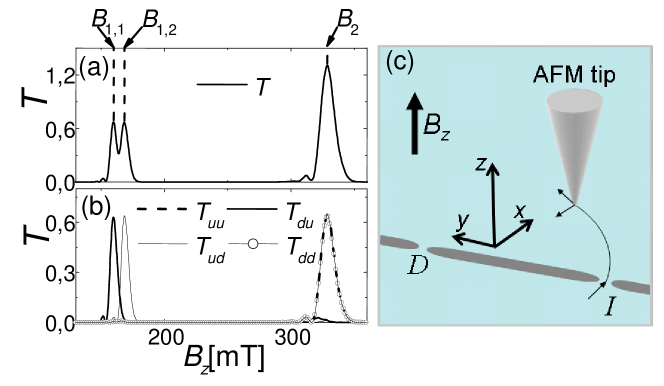
Figure 2: (a) Total focusing transmission coefficient $T$ versus applied perpendicular magnetic field $B_{z}$. (b) Spin resolved transmission coefficients versus $B_{z}$. We used $E_{F}\!=\!23$meV, $m^{*}\!=\!0.055m_{0}$, $\alpha\!=\!7$meVnm, $\beta\!=\!0$, $L\!=\!1.5\mu m$ and the width of the contacts is $70nm$. (c) Schematic of an SPM imaging procedure.

Here, we propose the use of this technique to explore the transverse focusing in the presence of spin-orbit interaction note2 . We simulate the effect of the tip potential by perturbing (increasing) the site energies $\varepsilon_{i,\sigma}$ in an area of the order of $100nm^{2}$ centered at the tip position. The Dyson equation is used to introduce the perturbation and the exact propagators between the contacts $I$ and $D$ are calculated for each position of the tip.

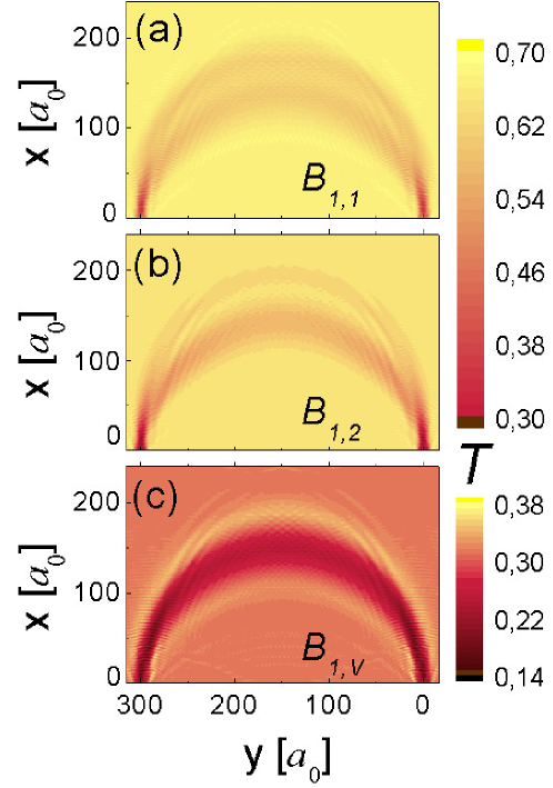
Figure 3: Total transmission coefficient $T$ between the contacts 1 and 2 as a function of the probe position for (a) $B_{z}\!=\!B_{1,1}$ , (b) $B_{z}\!=\!B_{1,2}$ and (c) $B_{z}\!=\!B_{1,v}\!=\!(B_{1,1}+B_{1,2})/2$. We used $\alpha\!=\!7$meVnm and the parameters given in Fig.2.

Figure 3.(a) shows $T$ vs the tip’s position when the perpendicular magnetic field is fixed to obtain the first maximum ($B_{z}\!=\!B_{1,1}$) for a SO coupling $\alpha\!=\!7$meVnm. The semicircular electron path is clearly observed. In this case the $T$ map is dominated by a drop in $T$ along the $O_{1}$ path. A similar pattern is found for the second transmission maximum ($B_{z}\!=\!B_{1,2}$) as shown in Fig.3.(b). In this case, the drop in $T$ is due to the scattering induced by the tip of electrons travelling along the $O_{2}$ path. A slightly different situation is found when $B_{z}$ is fixed in between $B_{1,1}$ and $B_{1,2}$ as shown in Fig.3.(c); although the variation is also dominated by a drop (dark area), $T$ increases at the two sides of the minimum. The observation of these two lobes shows that the tip, when placed at those positions, modifies the electron flow making a non-focalized electron path—$O_{1}$ or $O_{2}$ in Fig.1.(b)-(c)—to contribute to the transmission.

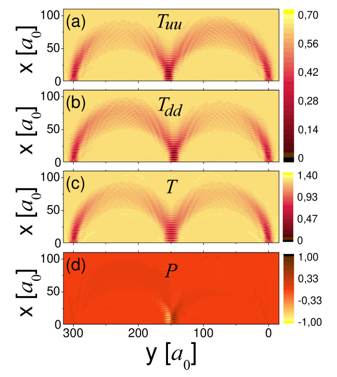
Figure 4: We plot (a) $T_{uu}$, (b) $T_{dd}$, (c) $T$ and (d) $P$ as a function of the probe position for $B_{z}\!=\!B_{2}$. We used $\alpha\!=\!7$meVnm and the parameters given in Fig.2.

More interesting are the imaging results obtained when the field is fixed at the second focusing condition: $B_{z}\!=\!B_{2}$. As mentioned above, in this case $T$ is dominated by the electron’s orbits with one bounce at the sample’s edge. For this field the largest contributions to the transmission coefficient are $T_{uu}$ and $T_{dd}$ , and the corresponding focusing peak is unsplit. In Fig.4 and Fig.5 the results for this case are shown for $\alpha\!=\!7$meVnm and $15$meVnm, respectively. Panel (a) shows $T_{uu}$ as a function of the position of the microscope probe. The change in the transmission in this case clearly shows that the electrons injected with spin $up$ (in the $y$-direction) leave the injector in the bigger orbit, rebound and then arrive to the detector in the smaller orbit with spin $up$—see $O_{2}$ in Fig.1(d). In panel (b) the transmittance $T_{dd}$ is shown —see $O_{1}$ in Fig.1(d) - and in panel (c) the total transmission coefficient is presented. As $T_{ud}$ and $T_{du}$ are very small, the total transmission is essentially given by the sum of the contributions shown in panels (a) and (b). Experimentally these two contributions could be distinguished by selecting the spin of the injected carriers. In fact, a combination of an external in-plane magnetic field in the $y$-direction and an appropriate gate voltage in the point contacts can be used to filter spins in the injector or detector PotokFMU02 . Selecting the spin of the injected electrons would make it possible to separate the two trajectories—(a) and (b) in Figs. 4 and 5—and obtain a direct visualization of the two orbits split by the spin-orbit coupling. Conversely, selecting the spin in the detector D, the transmissions $T_{+}=T_{uu}+T_{du}$ and $T_{-}=T_{ud}+T_{dd}$ of carriers arriving at $D$ with spin $up$ and $down$, respectively, could be measured. In terms of these quantities, we define the polarization $P$ of the transmitted particles as

$$P=\frac{T_{+}-T_{-}}{T}$$

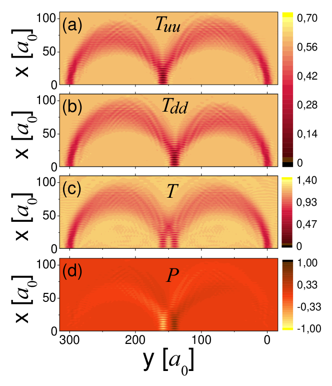
Figure 5: We plot (a) $T_{uu}$, (b) $T_{dd}$, (c) $T$ and (d) $P$ as a function of the probe position for $B_{z}\!=\!B_{2}$. We used $\alpha\!=\!15$meVnm and the parameters given in Fig.2.

Panel (c) and (d) of Figs. 4 and 5 show the total transmission coefficient $T\!$  and the polarization $P$ as a function of the tip position. The two semicircular electron paths including the rebound at the edge are visualized in the $T$ map. In our simulations the smaller and the bigger electron paths are not easily resolved in total transmission coefficient map except for the largest SO coupling case and for the tip close to the bounce position—see Fig.5(c). There, an appreciable fall (about $50\%$) of the transmission in the two rebound positions indicates that, when the probe is positioned there, the contribution to $T$ of one of the two possible electron paths ($O_{1}$ or $O_{2}$) is being suppressed. If $O_{1}$ is being suppressed, the electrons arriving to the detector will have spin $up$. On the other hand, if $O_{2}$ is suppressed only spin $down$ electrons will arrive to the detector. This means that one can select the spin polarization of the outgoing carrier flux by changing the tip position a few nanometers as shown in Fig.4(d) and Fig.5(d). Notably, the effect is also clearly observed in the case of the smaller SO coupling despite of the fact that the total transmittance $T$ does not resolve the two orbits.

4 Summary and Conclusions

We have discussed a microscopy imaging technique for the case transverse electron focusing in 2DEGs with strong Rashba coupling. The main results can be summarized as follows:

i.- The existence of two different cyclotron radii splits the first focusing peak onto two sub-peaks, each one corresponds to electrons arriving to the detector with different spin polarization along the direction parallel to the sample’s edge.

ii.- The images of the electron flow for focusing fields corresponding to the first two sub-peaks are very similar and consequently, for this case, the technique can not clearly distinguish the two type of orbits.

iii.- When the external field is fixed between the focusing fields of the two sub-peaks, $B_{z}=(B_{1,1}+B_{1,2})/2$, the transmission map shows a structure that indicates the presence of the two orbits.

iv.- For the second focusing condition, and for the case of strong Rashba coupling, the technique can resolve the two orbits when the microscope tip is placed close to the rebound position.

v.- For the case described in the previous point, the microscope tip can be used to polarize the electron flux arriving at the detector. The direction of the polarization can be reversed by changing the tip position a few nanometers.

Finally, we would like to emphasize a few points: a.- Interference fringes, characteristic of the quantum ballistic transport regime, are observed in all the $T$ maps; b.- For the properties studied here, replacing the hard wall potential $V(x)$ by a more realistic parabolic potential does not change the main properties of the system UsajB05_SHE ; GovorovKD04 . Therefore, our results should correctly describe the images that could be obtained in heterostructures defined by gates. c.- The competition between the Rashba and the Dresselhauss couplings leads to interesting features in the focusing signal and needs to be considered for interpreting imaging results in systems where these two SO interactions are present. These results will be presented elsewhere.

5 Acknowledgment

This work was supported by ANPCyT Grants No 13829 and 13476 and CONICET PIP 5254. AR acknowledge support from PITP and CONICET. GU is a member of CONICET.

References

- (1) D. Awschalom, N. Samarth, and D. Loss, eds., Semiconductor Spintronics and Quantum Computation (Springer, New York, 2002).
- (2) A. Reynoso, G. Usaj, and C. A. Balseiro, Phys. Rev. B 73, 115342 (2006).
- (3) R. Winkler, Spin-orbit coupling effects in two-dimensional electron and hole systems (Springer-Verlag, 2003).
- (4) J. Nitta, T. Akazaki, H. Takayanagi, and T. Enoki, Phys. Rev. Lett. 78, 1335 (1997).
- (5) M. Topinka, B. LeRoy, S. Shaw, E. Heller, R. Westervelt, K. Maranowski, and A. Gossard, Science (2000).
- (6) M. Topinka, B. LeRoy, R. Westervelt, S. Shaw, R.Fleischmann, E. Heller, K. Maranowski, and A. Gossard, Nature 410, 183 (2001).
- (7) G. Usaj and C. A. Balseiro, Phys. Rev. B 70, 041301(R) (2004).
- (8) Y. A. Bychkov and E. I. Rashba, JETP Letters 39, 78 (1984).
- (9) These are the solutions for positive . For negative the eingenstates change: .
- (10) A. Reynoso, G. Usaj, M. J. Sanchez, and C. A. Balseiro, Phys. Rev. B 70, 235344 (2004).
- (11) M. Pletyukhov, C. Amann, M. Mehta, and M. Brack, Phys. Rev. Lett. 89, 116601 (2002).
- (12) M. Gutzwiller, Chaos in Classical and Quantum Mechanics (Spring-Verlag, New York, 1991).
- (13) R. M. Potok, J. A. Folk, C. M. Marcus, and V. Umansky, Phys. Rev. Lett. 89, 266602 (2002).
- (14) L. P. Rokhinson, V. Larkina, Y. B. Lyanda-Geller, L. N. Pfeiffer, and K. W. West, Phys. Rev. Lett. 93, 146601 (2004).
- (15) H. van Houten, C. W. J. Beenakker, J. G. Willianson, M. E. I. Broekaart, P. H. M. Loosdrecht, B. J. van Wees, J. E. Mooji, C. T. Foxon, and J. J. Harris, Phys. Rev. B 39, 8556 (1989).
- (16) C. W. Beenakker and H. van Houten, in Solid State Physics, edited by H. Eherenreich and D. Turnbull (Academic Press, Boston, 1991), vol. 44, pp. 1–228.
- (17) D. K. Ferry and S. M. Goodnick, Transport in Nanostructures (Cambridge University Press, New York, 1997).
- (18) Imaging of cyclotron orbits using this imaging technique was reported at ICPS 28, Vienna (2006) by K. Aidala. See also AidalaPHW06 ; AidalaPHW07 .
- (19) G. Usaj and C. A. Balseiro, Europhys. Lett. 72, 631 (2005).
- (20) A. O. Govorov, A. V. Kalameitsev, and J. P. Dulka, Phys. Rev. B 70, 245310 (2004).
- (21) J. Schliemann and D. Loss, Phys. Rev. B 68, 165311 (2003).
- (22) K. E. Aidala, R. E. Parrott, E. Heller, and R. Westervelt, Int. J. Mod. Phys. A 21, 4407-4424 (2006).
- (23) K. E. Aidala, R. E. Parrott, Tobias Kramer, E. J. Heller, R. M. Westervelt, M. P. Hanson, and A. C. Gossard, Nat. Phys. 3, 464-468 (2007).