Phase diagram of the chromatic polynomial on a torus

Abstract

We study the zero-temperature partition function of the Potts antiferromagnet (i.e., the chromatic polynomial) on a torus using a transfer-matrix approach. We consider square- and triangular-lattice strips with fixed width $L$, arbitrary length $N$, and fully periodic boundary conditions. On the mathematical side, we obtain exact expressions for the chromatic polynomial of widths $L=5,6,7$ for the square and triangular lattices. On the physical side, we obtain the exact phase diagrams for these strips of width $L$ and infinite length, and from these results we extract useful information about the infinite-volume phase diagram of this model: in particular, the number and position of the different phases.

Key Words: Chromatic polynomial; antiferromagnetic Potts model; triangular lattice; square lattice; transfer matrix; Fortuin–Kasteleyn representation; Beraha numbers; conformal field theory.

1 Introduction

The two–dimensional (2D) $q$–state Potts model [1] is one of the most studied models in Statistical Mechanics. Despite many efforts over more than 50 years, its exact free energy and phase diagram are still unknown. The ferromagnetic regime of the Potts model is the best understood case: exact (albeit not always rigorous) results have been obtained for the ferromagnetic-paramagnetic phase transition temperature $T_{\rm c}(q)$ (at least for several regular lattices), the order of the transition (continuous for $0\leq q\leq 4$), the phase diagram, and the characterization in terms of conformal field theory (CFT) of the universality classes. (See e.g., Ref. [2].)

The antiferromagnetic regime is less understood, partly because universality is not expected to hold in general (in contrast with the ferromagnetic regime). We know the exact free energy along some curves of the phase diagram $(q,T)$ (where $T$ is the temperature) for some regular lattices [2]; but in this regime, this (partial) solubility of the model does not imply criticality (as it is been observed for the ferromagnetic regime with $0\leq q\leq 4$).

The standard $q$-state Potts model at temperature $T$ can be defined on any undirected finite graph $G=(V,E)$ as follows: on every vertex of the graph $x\in V$, we place a spin $\sigma_{x}$ taking an integer value in the set $\{1,2,\ldots,q\}$, where $q\in{\mathbb{N}}$. The spins interact via the Hamiltonian

$$\mathcal{H}_{\text{Potts}}(\{\sigma\})\;=\;-J\sum\limits_{\langle x,y\rangle\in E}\delta_{\sigma_{x},\sigma_{y}}$$ (1.1)

where the sum is over all edges $e=\langle x,y\rangle\in E$ joining nearest-neighbor sites, $J$ is the coupling constant, and $\delta$ is the Kronecker delta. The ferromagnetic (resp. antiferromagnetic) regime corresponds to $J>0$ (resp.  $J<0$). The partition function of the Potts model on a graph $G$ at inverse temperature $\beta=1/T\geq 0$ can then be written as

$$Z_{G}(q;J\beta)\;=\;\sum\limits_{\{\sigma\}}e^{-\beta\mathcal{H}_{\text{Potts}}}$$ (1.2)

A very useful representation of the Potts model is due to Fortuin and Kasteleyn [3]. They showed that the partition function (1.2) can be rewritten as

$$Z_{G}(q;v)\;=\;\sum\limits_{E^{\prime}\subseteq E}q^{k(E^{\prime})}\,v^{|E^{\prime}|}$$ (1.3)

where $v=e^{J\beta}-1$, the sum is over the $2^{|E|}$ spanning subgraphs $(V,E^{\prime})$ of $G$, and $k(E^{\prime})$ is the number of connected components (including isolated vertices) of the spanning subgraph $(V,E^{\prime})$. As a result, the partition function (1.3) is a polynomial in both variables $q$ and $v$. Thus, we can promote (1.3) to the definition of the model, which allows us to consider $q$ as an arbitrary complex number.

We shall here focus on the zero-temperature antiferromagnetic case $J=-\infty$ (i.e., $v=-1$), whose restriction to $q\in{\mathbb{N}}$ can be interpreted as a coloring problem. In this case, $P_{G}(q)=Z_{G}(q,-1)$ is known as the chromatic polynomial of $G$. Its evaluation for a general graph is a hard problem. More precisely, Oxley and Welsh have proven that the computation of the coefficients $a_{k}$ of the chromatic polynomial $P_{G}(q)=\sum_{k=1}^{|V|}a_{k}\,q^{k}$ of a general graph $G$ (including bipartite graphs) is #-P hard [4].

In this paper, we will consider only strip graphs of certain regular lattices (i.e., square and triangular). For a family of strip graphs $\{G_{n}\}$ (or, more generally, recursive families of graphs [5]), the chromatic polynomial $P_{G_{n}}(q)$ of any member of the family $G_{n}$ can be computed from a transfer matrix ${\mathsf{T}}$ and certain boundary condition vectors $\bm{u}$ and $\bm{v}$:

$$P_{G_{n}}\;=\;\bm{u}^{\text{T}}\cdot{\mathsf{T}}^{n}\cdot\bm{v}\,.$$ (1.4)

Thus, the computation time grows as a polynomial in $n$ for fixed strip width $L$. However, it still grows exponentially in the strip width (due to the $L$ dependence of $\dim{\mathsf{T}}$). It is therefore of interest to devise new and efficient algorithms to be able to handle as large widths $L$ as possible.

Remark. It is important to stress that the Potts spin model has a probabilistic interpretation (i.e., has non-negative Boltzmann weights) only when $q$ is a positive integer and $v\geq-1$ (i.e., positive temperature). The Fortuin-Kasteleyn random-cluster model (1.3), which extends the Potts model to non-integer $q$, has non-negative weights only when $q,v\geq 0$. In all other cases, the model belongs to the “unphysical” regime (i.e., some weights are negative or complex), and some familiar properties of statistical mechanics need not hold. For example, even for integer $q\geq 2$ and real $v$ in the antiferromagnetic range $-1\leq v<0$, where the spin representation exists and has non-negative weights, the dominant eigenvalue $\lambda_{\star}$ of the transfer matrix in the cluster representation need not be simple (i.e., the eigenvector may not be unique); and even if simple, it may not play any role in determining $Z_{G_{n}}(q,v)$ because the corresponding amplitude may vanish. Both these behaviors are of course impossible for any transfer matrix with positive weights, by virtue of the Perron-Frobenius theorem. It is important to note that the dominant eigenvalues in the cluster and spin representations need not be equal, because the former may have a vanishing amplitude (see below). In any case, the Potts model can thus make probabilistic sense in the cluster representation at parameter values where it fails to make probabilistic sense in the spin representation, and vice versa. It is worth mentioning that for $q=4\cos^{2}(\pi/n)$ with integer $n\geq 3$ and planar graphs $G$, the Potts-model partition function $Z_{G}(q,v)$ admits a third representation, in terms of a restricted solid-on-solid (RSOS) model [6, 7] (See also Ref. [8] for an recent study with a more comprehensive list of references).

Even though the zero-temperature limit of the Potts antiferromagnet may not have a probabilistic interpretation in the Fortuin–Kasteleyn representation [3] for non-integer $q$, it can nevertheless being studied with the standard tools of Statistical Mechanics and CFT with appropriate modifications. In particular, we expect that critical “unphysical regions” can be described with non-unitary field theories. (See [10, 9] for a more detailed discussion on these points.)

It is well established that antiferromagnetic models in general, and the chromatic polynomial in particular, are very sensitive to the choice of boundary conditions. Indeed, different choices may lead to quite different thermodynamic limits. In our earlier publications [11, 12, 13] we studied free and cylindrical boundary conditions: free boundary conditions in the longitudinal direction and free or periodic boundary conditions in the transverse direction, respectively. More recently [9], we considered cyclic boundary conditions: namely, free boundary conditions in the transverse direction, and periodic boundary conditions in the longitudinal direction. In particular, we observed that in the latter case, the phase diagram of the triangular-lattice chromatic polynomial was more involved than for free or cylindrical boundary conditions. In this paper we shall deal with fully periodic boundary conditions (i.e., periodic in both directions). Periodic boundary conditions in the longitudinal direction (i.e., toroidal and cyclic) can be easily implemented in the spin representation as $P_{G_{n}}=\mathop{\rm tr}\nolimits{\mathsf{T}}^{n}$. In the Fortuin-Kasteleyn representation, this implementation is less obvious as shown in Ref. [9]. For the triangular-lattice model with periodic boundary conditions on the transverse direction we should also use some additional tricks [14, 11, 13].

The results existing in the literature about exact chromatic polynomials for strips of the square and triangular lattices with toroidal boundary conditions are limited to $L\leq 4$. The earlier results were obtained by recursive use of the contraction-deletion theorem. These works include the pioneering paper by Biggs, Damerell, and Sands [15] (where the solution for a square-lattice strip of width $L=2$ was presented), and those of Chang and Shrock [16, 17, 18]. In Ref. [17] the latter authors gave the exact solution for the full Potts-model partition function (i.e., with arbitrary $v$) for square-lattice strips of widths $L=2,3$. In Ref. [18] the solution for the triangular-lattice chromatic polynomial for width $L=3$ was presented, while in Ref. [16] they gave the solution for both lattice strips of width $L=4$. Finally, in 2006 Chang and Shrock exhibited a transfer-matrix formalism to compute the full Potts-model partition function for regular lattice strips with toroidal boundary conditions [19]. In particular, they gave the exact partition function for square-lattice strips of widths $L\leq 4$, and triangular-lattice strips of widths $L=2,3$. In Ref. [19], they also obtained structural properties of the partition function and the chromatic polynomial. Additional structural properties were discussed by one of us [20].

We have several motivations for this work. As explained above, the exact solution of the 2D $q\neq 2$ state Potts model at general $v$ is still unknown, even for the square lattice (and a fortiori for more complicated regular lattices), and even in the thermodynamic limit (and a fortiori on general finite lattices). Therefore, exact solutions of this model on strips of finite fixed width and arbitrary length are valuable in their own right (even in the particular case $v=-1$). In addition, the chromatic polynomial $P_{G}(q)$ is an object of great interest to mathematicians (see e.g., Ref. [21] for a recent survey). As the computation of the chromatic polynomial is #–P hard [4], new and efficient methods for computing this object on large graphs are also of great interest to this community.

The second motivation of this work is to deepen our physical understanding of the critical points of the $q$-state Potts model in the antiferromagnetic $-1\leq v<0$ and unphysical regimes $v<-1$. Indeed, we can extract this information from our finite-width strips using CFT and finite-size scaling (FSS) [22, 23, 24]. In particular, we will consider the following way to attain the thermodynamic limit. From the chromatic polynomial of a strip of size $L\times N$ we can compute its chromatic zeros in the complex $q$-plane. From these zeros it is very hard to obtain infinite-volume quantities, as they have strong FSS corrections. Thus, we consider the infinite-length limit $N\to\infty$. Then, the chromatic zeros accumulate along certain limiting curves $\mathcal{B}_{L}$ and around isolated limiting points. This phenomenon is a consequence of the Beraha–Kahane–Weiss theorem [25]. Our methods allow us to obtain the exact values of the relevant physical quantities in this limit. Their FSS corrections are found to be smaller than when both $L$ and $N$ are finite. The extrapolation to the true infinite-volume limit $L\to\infty$, using standard FSS techniques, therefore becomes more precise by employing this order of limits.

Remark. Toroidal boundary conditions are rather special compared to the other boundary conditions studied in previous papers: namely, free, cylindrical, and cyclic [11, 12, 13, 9]. Strip graphs with the latter boundary conditions are planar; thus, the four-color theorem [26] applies. However, strip graphs with the former boundary conditions can be regarded as graphs embedded on a torus. In this case, we have only a seven-color theorem. This follows from the upper bound obtained by Heawood [27] in 1890 on the chromatic number of a graph $G$ embedded on an orientable surface of genus $g\geq 1$

$$\chi(G)\;\leq\;H(g)\;=\;\left\lfloor\frac{1}{2}\left(7+\sqrt{1+48g}\right)\right\rfloor$$ (1.5)

combined with the fact that $K_{7}$ (with $\chi(K_{7})=7$) can be embedded on a torus, as shown in Figure 1. Ringel and Youngs [28] finally proved that the maximum chromatic number of any graph $G$ on an orientable surface of genus $g\geq 1$ is given by $H(g)$. This graph-theoretic difference between graphs embedded on a surface or on a torus may have physical implications that are worth studying: in particular, is there any additional structure (e.g., phase-transition lines) in the interval $q\in(4,7)$ for the chromatic polynomial of a strip graph embedded on a torus?

The main part of our physical (as opposed to mathematical) understanding of the mechanism for generating chromatic zeros stems from Saleur’s analysis of the so-called Berker–Kadanoff (BK) phase [29]. This is a massless phase with algebraic decay of correlations. For the square lattice, this phase is bounded by the curves

$$v_{\pm}(q)\;=\;-2\pm\sqrt{4-q}$$ (1.6)

and all this region is attracted (at fixed $q$) by the curve

$$v(q)\;=\;-\sqrt{q}\,,\qquad q\in[0,4]$$ (1.7)

It is important to stress four points here: First, the BK phase corresponds to generic values of $q\in(0,4)$. More precisely, for the Beraha numbers $B_{p}$

$$B_{p}\;=\;4\cos^{2}\left(\frac{\pi}{p}\right)\,,\qquad p\in{\mathbb{N}}\,,\quad p\geq 2$$ (1.8)

the BK phase does not exists due to the vanishing of the amplitude of some of the leading eigenvalues and/or cancellations among them [29, 30]. Second, the chromatic-polynomial subspace $v=-1$ intersects the BK phase for $q\in[0,3]$. Thus, because of the attractive nature of the BK critical curve (1.7), we can study its conformal properties by considering the chromatic-polynomial case in the window $q\in[0,3]$. Third, the upper boundary of the BK phase $v_{+}(q)$ (1.6) can be identified as the antiferromagnetic critical curve [31]. Fourth, the exact free energy of the chromatic-polynomial line is not known. However, from our previous studies [11, 12, 9], we can draw a qualitative picture of the chromatic-polynomial phase diagram for real $q$: the system is disordered in the region $q\in(-\infty,0)\cup(3,\infty)$, while it is critical in the interval $q\in(0,3)$. The nature of the system in this critical interval depends on the boundary conditions: for free and cylindrical boundary conditions there is a single phase [11, 12]; but for cyclic boundary conditions, we find two different phases: the intervals $q\in(0,2)$, and $q\in(2,3)$ corresponding to two distinct values of a topological order parameter (See Section 2.2) [9]. If we define the value $q_{c}$ as the largest value of $q$ such that the system is disordered for all $q>q_{c}$ and the system is critical at $q=q_{c}$ [32], then for the square lattice we have that $q_{c}(\text{sq})=3$ [33].

The situation for the triangular lattice is slightly different. This model is solvable on the curve [34]

$$v^{3}+3v^{2}\;=\;q$$ (1.9)

The lower branch of the curve (1.9) can be identified with the lower bound of the BK phase $v_{-}(q)$, while the middle branch of (1.9) is expected to play the same role as the curve (1.7) [i.e., it is the renormalization-group (RG) attractor governing the BK phase]. Thus, for the triangular lattice at least one curve is missing (if we assume a RG flow similar to that of the square lattice): the upper bound of the BK phase [i.e., the analogue of the curve $v_{+}(q)$ (1.7)], and the antiferromagnetic critical curve. In the limit $q\to 0$, we have found [10] that there is a single phase-transition line separating the (critical) BK phase and the (non-critical) high-temperature phase. This line is interpreted as the antiferromagnetic critical curve for this model, and its slope is given approximately by

$$\left.\frac{{\rm d}v}{{\rm d}q}\right|_{q=0}\;=\;-0.1753\pm 0.0002$$ (1.10)

The position of these two curves is an open problem (Some preliminary numerical results about the antiferromagnetic critical curve were published in [10, Figure 2]. The full curve will be published elsewhere [35]). Theoretical [30] and numerical [10] studies show that the BK phase does exist in the triangular-lattice model, and the results suggest that universality holds for this phase (i.e., the critical properties of the square- and triangular-lattice BK phase coincide).

Even though some important curves of the phase diagram of the triangular-lattice chromatic polynomial are not known, Baxter [14] found its exact free energy, albeit with peculiar boundary conditions that amount to not giving a weight $q$ to clusters with non-trivial homotopy. We comment further on that solution in Sections 5–6 (see also Ref. [13]). The resulting phase diagram consists of three different phases in the complex $q$-plane: the disordered phase contained the interval $q\in(-\infty,0)\cup(4,\infty)$, and there are two critical phases. One contains the interval $q\in(0,q_{2}(\text{tri}))$, where $q_{2}(\text{tri})$ is given by

$$q_{2}(\text{tri})\;=\;q_{\text{B}}\;\simeq\;3.8196717312$$ (1.11)

and the third one contains the interval $q\in(q_{2}(\text{tri}),4)$. From this phase diagram, we obtain that $q_{c}(\text{tri})=4$.

Our previous studies [13, 9], gave a similar qualitative picture of that phase diagram. In these papers, we have defined $q_{0}(L)$ as the largest value of $q$ at which the limiting curve $\mathcal{B}_{L}$ crosses the real $q$-axis. We expect that the limit $q_{0}=\lim_{L\to\infty}q_{0}(L)$ exists, and it is equal to $q_{2}(\text{tri})$. In Ref. [13] we reanalyzed Baxter’s solution and found that if his three analytical expressions for the free energy are correct and exhaustive, the phase transition should not occur at $q_{2}(\text{tri})=q_{\text{B}}$, but rather at

$$q_{2}(\text{tri})\;=\;q_{\text{G}}\;=\;2+\sqrt{3}\;\approx\;3.7320508076$$ (1.12)

Unfortunately, our numerical data were not conclusive enough to judge which is the correct value of the transition point. For free and cylindrical boundary conditions [13], the corresponding phase diagram contains only the above three phases. For cyclic boundary conditions [9], we found a richer phase structure within the interval $q\in(0,4)$. In particular, in the interval $q\in(0,q_{2}(\text{tri}))$, there should be phase transitions at the Beraha numbers $q=B_{4},B_{6},\ldots\leq q_{2}({\rm tri})$ [cf. Eq. (1.8)]. If $q_{2}(\text{tri})=q_{\text{B}}$, then the last such transition occurs at $q=B_{14}\approx 3.8019377358$; but if $q_{2}(\text{tri})=q_{\text{G}}$, then the last transition is at $q=B_{12}=q_{\text{G}}$.

Finally, the chromatic-polynomial line $v=-1$ has a non-void intersection with the BK phase for the triangular lattice. In particular, we expect that the intersection should include the whole interval $q\in(0,q_{2}(\text{tri}))$. Thus, the critical properties extracted from this interval are related directly to those of the BK phase. In the interval $q\in(q_{2}(\text{tri}),4)$, the universality class should be different from that of the BK phase. For other boundary conditions, we have been unable to extract any meaningful physical information for this interval; so this question remains open. In the ferromagnetic regime, it is well-known that results obtained from toroidal boundary conditions are closer to the true thermodynamic limit that for the other boundary conditions. Although the argument leading to this conclusion may not apply for antiferromagnetic or “unphysical” models, it opens an opportunity to try to answer the above-posed questions.

This paper is organized as follows: in Section 2 we show in detail how to obtain the chromatic polynomial of a strip with toroidal boundary conditions, and some structural properties: dimensionality of the transfer matrix and properties of the amplitudes. Sections 3 and 4 contain the detailed description (when possible) of the chromatic polynomial for square- and triangular-lattice strips, respectively. In these two sections we also describe the limiting curve for each regular lattice. The less-mathematically inclined readers can skip most of these sections. In Section 5 we discuss the finite-width results and extract the physically interesting quantities: phase diagram of the chromatic polynomial for the square and triangular lattices, and critical properties of the different phases. Finally, in Section 6, we draw our conclusions. In Appendix A we prove two useful combinatorial identities needed in Section 2.2.

2 Chromatic polynomials with toroidal boundary conditions

We want to build the transfer matrix for square- and a triangular-lattice strips of width $m$ and arbitrary length $n$ with toroidal boundary conditions. The goal is to write the transfer matrix ${\mathsf{T}}(m)$ as a product of two matrices

$${\mathsf{T}}(m)\;=\;{\mathsf{H}}(m)\cdot{\mathsf{V}}(m)$$ (2.1)

where ${\mathsf{H}}$ (resp. ${\mathsf{V}}$) represents the horizontal (resp. vertical) bonds of the lattice, and to write its chromatic polynomial in the form

$$P_{m_{\text{P}}\times n_{\text{P}}}(q)\;=\;\bm{u}^{\text{T}}\cdot{\mathsf{H}}(m)\cdot{\mathsf{T}}(m)^{n}\cdot\bm{v}_{\text{id}}$$ (2.2)

for some left and right vectors $\bm{u}$ and $\bm{v}_{\text{id}}$. The subindex P denotes the periodic boundary condition in the corresponding direction.

2.1 The transfer-matrix formalism for toroidal boundary conditions

The main problem in writing a transfer matrix in the Fortuin-Kasteleyn representation is the non-local factor $q^{k(E^{\prime})}$ in (1.3) [11]. For free boundary conditions in the longitudinal direction (i.e., free and cylindrical), this can be efficiently handled by keeping track of the connectivity state $\bm{v}_{\mathcal{P}}$ of the top layer. This connectivity is related to a certain partition $\mathcal{P}$ of the single-layer vertex set $\{1,2,\ldots,m\}$ [11, 13].

For periodic boundary conditions in the longitudinal direction (i.e., cyclic and toroidal) we must keep track of the connectivity state of both the top and bottom rows: each connectivity state $\bm{v}_{\mathcal{P}}$ is now given by a certain partition $\mathcal{P}$ of the vertex set of the top row $\{1,2,\ldots,m\}$ and the vertex set of the bottom row $\{1^{\prime},2^{\prime},\ldots,m^{\prime}\}$. In Figure 2 we show an example of a square-lattice strip of size $4\times 2$. As for cyclic boundary conditions [9], initially the top and bottom rows are identical. Then, we enlarge the strip by adding new layers via the action of the transfer-matrix operator ${\mathsf{T}}(m)$ exclusively on the top-row vertices (while the bottom-row sites remain unchanged). At the end, when we have built a strip of $n+1$ rows, we identify the top and bottom rows.

Let us now explain in more detail how to obtain the chromatic polynomial for a square-lattice strip of width $m$, length $n$, and toroidal boundary conditions.

We characterize the state of the top and bottom rows by a connectivity state $\bm{v}_{\mathcal{P}}$, which is associated to a partition $\mathcal{P}=\{\mathcal{P}_{1},\mathcal{P}_{2},\ldots,\mathcal{P}_{k}\}$ of the set $\{1,2,\ldots,m,1^{\prime},2^{\prime},\ldots,m^{\prime}\}$. We then introduce the operators

$${\mathsf{P}}_{x}&=vI+{\mathsf{D}}_{x}{}\\ {\mathsf{Q}}_{x,y}=I+v{\mathsf{J}}_{x,y}{}$$ (2.3)

acting on the connectivity space $\{\bm{v}_{\mathcal{P}}\}$. Here $I$ is the identity, ${\mathsf{D}}_{x}$ is the detach operator that detaches site $x$ from the block it currently belongs to, and ${\mathsf{J}}_{x,y}$ is the join operator that amalgamates the blocks containing sites $x$ and $y$, if they were not already in the same block. (Further details can be found in Ref. [11].)

The matrices ${\mathsf{V}}$ and ${\mathsf{H}}$ are defined in terms of the above operators as follows:

$${\mathsf{H}}_{\text{sq}}(m)&=\left(\prod\limits_{i=1}^{m-1}{\mathsf{Q}}_{i,i+1}\right)\cdot{\mathsf{Q}}_{m,1}{}\\ {\mathsf{V}}_{\text{sq}}(m)=\prod\limits_{i=1}^{m}{\mathsf{P}}_{i}{}$$ (2.4)

Notice that periodic boundary conditions have been implemented by adding the operator ${\mathsf{Q}}_{m,1}$ in (LABEL:def_Hsq). We can similarly define a matrix ${\mathsf{H}}^{\prime}_{\text{sq}}$ acting only on the bottom row.

Then, the chromatic polynomial for a square-lattice strip of size $m\times n$ with toroidal boundary conditions can be written as in (2.1)/(2.2), where the two vectors are those of cyclic boundary conditions [9]. The vector $\bm{v}_{\text{id}}$ denotes the partition

$$\bm{v}_{\text{id}}\;=\;\{\{1,1^{\prime}\},\{2,2^{\prime}\},\ldots,\{m,m^{\prime}\}\}$$ (2.5)

(i.e., we start with the top and bottom rows identified). The left vector $\bm{u}^{\text{T}}$ acts on a connectivity state $\bm{v}_{\mathcal{P}}$ as

$$\bm{u}^{\text{T}}\cdot\bm{v}_{\mathcal{P}}\;=\;q^{|\mathcal{P}^{\prime}|}$$ (2.6)

where $|\mathcal{P}^{\prime}|$ denotes the number of blocks in the connectivity state $\bm{v}_{\mathcal{P}}^{\prime}$ obtained from $\bm{v}_{\mathcal{P}}$ by

$$\bm{v}_{\mathcal{P}}^{\prime}\;=\;\left(\prod\limits_{i=1}^{m}{\mathsf{J}}_{i,i^{\prime}}\right)\cdot\bm{v}_{\mathcal{P}}$$ (2.7)

Thus, $\bm{u}^{\text{T}}$ acts on $\bm{v}_{\mathcal{P}}$ by identifying the top and bottom rows, and then by assigning a factor of $q$ to each block in the resulting partition.

The definition of the transfer matrix for a triangular-lattice strip of width $m$, length $n$, and toroidal boundary conditions is more involved because of the periodic boundary conditions in the transverse direction. As explained in Refs. [11, 13], in this case one has to consider a triangular lattice of width $m+1$ with free boundary conditions in the transverse direction, and then identify the columns $1$ and $m+1$. (See Figure 3 for an example of size $4\times 2$.) Then, the matrices ${\mathsf{H}}$ and ${\mathsf{V}}$ take the form

$${\mathsf{H}}_{\text{tri}}(m)&=\left(\prod\limits_{i=1}^{m}{\mathsf{Q}}_{i,i+1}\right)\cdot{\mathsf{J}}_{m+1,1}{}\\ {\mathsf{V}}_{\text{tri}}(m)=\left(\prod\limits_{i=1}^{m}{\mathsf{P}}_{i}\cdot{\mathsf{Q}}_{i,i+1}\right)\cdot{\mathsf{P}}_{m+1}{}$$ (2.8)

where the operators ${\mathsf{Q}}_{i,i+1}$ in (LABEL:def_Vtri) represent the oblique bonds $e=\langle(i,j+1),(i+1,j)\rangle$. With this definitions, the chromatic polynomial can be written as in (2.1)/(2.2) with the same right and left vectors as for the square-lattice case (2.5)/(2.6).

A further simplification can be obtained if we take into account the fact that $v=-1$. Then, ${\mathsf{H}}$ is a projector (i.e., ${\mathsf{H}}^{2}={\mathsf{H}}$), and we can use instead of the transfer matrix ${\mathsf{T}}$ and the basis vectors $\bm{v}_{\mathcal{P}}$, the modified transfer matrix ${\mathsf{T}}^{\prime}$

$${\mathsf{T}}^{\prime}(m)\;=\;{\mathsf{H}}(m)\cdot{\mathsf{V}}(m)\cdot{\mathsf{H}}(m)$$ (2.9)

and the modified basis vectors

$$\bm{w}_{\mathcal{P}}\;=\;{\mathsf{H}}(m)\cdot\bm{v}_{\mathcal{P}}$$ (2.10)

Note that $\bm{w}_{\mathcal{P}}=0$ if $\mathcal{P}$ has any pair of nearest-neighbor sites of the top row in the same block. Thus, the space $\{\bm{w}_{\mathcal{P}}\}$ has lower dimension than the original connectivity space $\{\bm{v}_{\mathcal{P}}\}$.

Notice that we start with the state $\bm{w}_{\text{id}}={\mathsf{H}}\cdot\bm{v}_{\text{id}}$, and that at the end we identify the top and bottom rows. Then, it is very useful to work directly with the modified connectivity basis

$$\widehat{\bm{w}}_{\mathcal{P}}\;=\;{\mathsf{H}}^{\prime}(m)\cdot{\mathsf{H}}(m)\cdot\bm{v}_{\mathcal{P}}$$ (2.11)

This choice implies that $\widehat{\bm{w}}_{\mathcal{P}}=0$ also if $\mathcal{P}$ contains any pair of nearest-neighbor sites of the bottom row in the same block. For simplicity, we will drop hereafter the prime in the modified transfer matrix (2.9) and the hat in the modified basis vectors (2.11). Then, the chromatic polynomial can be written as

$$P_{m_{\text{P}}\times n_{\text{P}}}(q)\;=\;\bm{u}^{\text{T}}\cdot{\mathsf{T}}(m)^{n}\cdot\bm{w}_{\text{id}}$$ (2.12)

Finally, to lighten the notation, we will write the connectivity states $\bm{v}_{\mathcal{P}}$ using Kronecker delta-functions. For instance, $\bm{v}_{\{\{1,2\},\{1^{\prime},3^{\prime}\},\{3\},\{2^{\prime}\}\}}$ will be written as $\delta_{1,2}\delta_{1^{\prime},3^{\prime}}$. The identity connectivity state (2.5) will be denoted simply as $1$.

2.2 Structural properties of the chromatic polynomial

Our first goal is to compute the number $C_{m,m}$ of non-crossing connectivities in the interior of an annulus with $m$ points on the inner rim and $m$ points on the outer rim (See Figure 4). This problem can be reduced to a simpler one by introducing the quantities $d(m,\ell)$. Given $m$ points on a circle and a non-crossing connectivity ${\cal P}$ exterior to that circle, we can compute the number of ways $d(m,\ell,{\cal P})$ we can connect that particular connectivity ${\cal P}$ to infinity by means of $\ell$ mutually non-connected paths (bridges). Then, the $d(m,\ell)$ are the sum over all possible connectivities ${\cal P}$

$$d(m,\ell)=\sum\limits_{{\cal P}}d(m,\ell,{\cal P})$$ (2.13)

The values of $d(m,\ell)$ are given by the following formula [19]

$$d(m,\ell)\;=\;\begin{cases}\qquad C_{m}&\qquad\text{if $\ell=0$}\\[14.22636pt] \qquad\displaystyle\binom{2m-1}{m-1}&\qquad\text{if $\ell=1$}\\[14.22636pt] \qquad\displaystyle\binom{2m}{m-\ell}&\qquad\text{if $2\leq\ell\leq m$}\\[14.22636pt] \qquad 0&\qquad\text{if $\ell>m$}\end{cases}$$ (2.14)

where $C_{m}$ is the Catalan number

$$C_{m}=\frac{1}{m+1}\,\binom{2m}{m}$$ (2.15)

which gives the number of non-crossing connectivities with $m$ points on a circle (or on a line).

The number of connectivities $C_{m,m}$ can be obtained easily from the $d(m,\ell)$ (2.14) by using the $\ell$ paths as bridges and by matching two such bridge connectivities with the same value of $0\leq\ell\leq m$

$$C_{m,m}\;=\;C_{m}^{2}+\sum\limits_{\ell=1}^{m}\ell\,d(m,\ell)^{2}$$ (2.16)

If we insert (2.14) for the $d(m,\ell)$, then we obtain a closed expression for $C_{m,m}$:

$$C_{m,m}\;=\;\frac{m^{2}-2m+5}{m+1}\,\binom{2m-1}{m}^{2}$$ (2.17)

where we have used the identity (LABEL:lemma1) proven in Appendix A. The asymptotic growth of $C_{m,m}$ as $m\to\infty$ is exponentially fast with a large constant:

$$C_{m,m}\;\sim\;\frac{16^{m}}{4\pi}\left[1+O\left(\frac{1}{m}\right)\right]\,,\quad\text{as $m\to\infty$}$$ (2.18)

In practice, we build the $C_{m,m}$ non-crossing connectivities in a recursive way. We start with all the $C_{m-1,m-1}$ non-crossing connectivities on an annulus with $m-1$ points on its inner and outer rims, and then we add a new site on the inner rim. The number of non-crossing connectivities for this annulus is obtained again by matching the $\ell$-bridge connectivities

$$C_{m,m-1}\;=\;C_{m}\,C_{m-1}+\sum\limits_{\ell=1}^{m-1}\ell\,d(m,\ell)\,d(m-1,\ell)$$ (2.19)

Then, we add a new site on the outer rim, and we obtain the $C_{m,m}$ connectivities (2.17). A closed formula for $C_{m,m-1}$ (2.19) can be obtained if we use the combinatorial identity (LABEL:lemma2) proven in Appendix A. After some algebra, we obtain

$$C_{m,m-1}\;=\;\frac{2m^{4}-6m^{3}+11m^{2}+3m-4}{2m^{2}(m+1)}\,\binom{2m-2}{m-1}^{2}$$ (2.20)

valid for all $m\geq 2$. This formula also grows exponentially fast in $m$ in the large-$m$ limit:

$$C_{m,m-1}\;\sim\;\frac{16^{m}}{16\pi}\left[1+O\left(\frac{1}{m}\right)\right]\,,\quad\text{as $m\to\infty$}$$ (2.21)

In Table 1 we show the values of $C_{m,m}$ and $C_{m,m-1}$ for $1\leq m\leq 7$.

The condition $v=-1$ implies that connectivities $\mathcal{P}$ containing nearest-neighbor sites in any sub-block do not contribute. The number of non-crossing non-nearest-neighbor connectivities for an annulus with $m$ points on its inner and outer rims will be denoted by $D_{m,m}$. This number gives therefore the dimension of the modified transfer matrix (2.9) for a square- or triangular-lattice strip of width $m$ and toroidal boundary conditions. These numbers are displayed for $1\leq m\leq 7$ in Table 1.

As in previous works [11, 12, 13, 9], we can reduce this dimension by considering the equivalence classes modulo symmetries of non-crossing non-nearest-neighbor connectivity states. For the triangular (resp. square) lattice, we should consider equivalence classes modulo rotations (resp. rotations and reflections with respect to any diameter of the strip). The number of generated equivalence classes modulo rotations (resp. reflections and rotations) of non-crossing non-nearest-neighbor connectivity states for a strip of width $m$ will be denoted by TriTorus${}^{\prime}(m)$ (resp.  SqTorus${}^{\prime}(m)$). The adjective “generated” means that we only take into account those classes of connectivity states that can be produced by applying the various operators ${\mathsf{P}}_{i}$ and ${\mathsf{Q}}_{i,j}$ on the right vector $\bm{w}_{\text{id}}$. This distinction is relevant for the square lattice, as there are perfectly legal non-crossing non-nearest-neighbor partitions that cannot be generated when we start from the right vector $\bm{w}_{\text{id}}$. (See e.g., the discussion on this issue in Ref. [20, end of Section 2.1].) The simplest example corresponds to $m=2$ and the connectivity state $\delta_{2,1^{\prime}}\delta_{1,2^{\prime}}$. In general, out of the $m$ possible connectivity states with $\ell=m$ bridges, only the state $\bm{v}_{\text{id}}$ (2.5) can be realized on a square-lattice strip. The other $m-1$ non-crossing connectivity states cannot be realized because of the lattice structure. However, on the triangular lattice, which has a larger set of “vertical” edges, one can produce those $m-1$ connectivity states without violating the non-crossing condition.

Finally, as for cyclic boundary conditions, for a given width $m$ we find many repeated eigenvalues. Thus, we define TriTorus$(m)$ (resp. SqTorus$(m)$) as the number of distinct eigenvalues (with non-zero amplitude) for a triangular-lattice (resp. square-lattice) strip of width $m$ with fully periodic boundary conditions. In Table 1 we have displayed the quantities TriTorus^′, SqTorus^′, TriTorus and SqTorus for $m\leq 7$ (when available).

The symbolic computation of the transfer matrix and the $\bm{u}^{\text{T}}$ and $\bm{w}_{\text{id}}$ vector has been carried out using a mathematica script for the smallest widths $2\leq m\leq 4$, and a C program for the larger widths $m\leq 7$. Indeed, for $m\leq 4$, both methods perfectly agree. We refer to Refs. [12, 13, 9] for details about the symbolic computation. For larger widths $m\leq 15$, we have computed numerically the transfer matrix using another C program.

Remarks. 1) With our transfer-matrix approach we have checked all previous results by Biggs, Damerell and Sands [15], and Chang and Shrock [16, 17, 18, 19].

2) Even though the final dimensions of the transfer matrices are TriTorus${}^{\prime}(m)$ or SqTorus${}^{\prime}(m)$, the actual computations are carried out in the larger space of non-crossing connectivities (of dimension $C_{m,m}$). This fact limits the maximum width we are able to handle.

3) We have cross-checked our results using the trivial identity

$$P_{m_{\text{P}}\times n_{\text{P}}}(q)\;=\;P_{n_{\text{P}}\times m_{\text{P}}}(q)$$ (2.22)

for all $2\leq m,n\leq 7$.

2.3 Amplitudes for toroidal boundary conditions

The transfer matrix for a strip with toroidal boundary conditions has a block structure. This property also holds for cyclic boundary conditions [9], and in both cases the origin is the same. Given a certain connectivity $\mathcal{P}$ of the top and bottom rows (see e.g., Figure 4), we can regard it as a bottom-row connectivity $\mathcal{P}_{\text{bot}}$, a top-row connectivity $\mathcal{P}_{\text{top}}$ joined by $\ell$ bridges. Notice that each top-row block can be connected to a bottom-row block by at most one bridge, and vice versa. Thus, the number of bridges is an integer $0\leq\ell\leq m$.

As explained in Ref. [9], the full transfer matrix has a lower-triangular block form (if we order the connectivity states in decreasing order of bridges).

$${\mathsf{T}}(m)\;=\;\left(\begin{array}[]{cccc}T_{m,m}&0&\ldots&0\\ T_{m-1,m}&T_{m-1,m-1}&\ldots&0\\ \vdots&\vdots&&\vdots\\ T_{0,m}&T_{0,m-1}&\ldots&T_{0,0}\end{array}\right)$$ (2.23)

The reason is the application of the ${\mathsf{H}}$ and ${\mathsf{V}}$ operators cannot increase the number of bridges of a given connectivity state. Furthermore, as the transfer matrix does not act on the bottom-row connectivity and they act on the space of non-crossing connectivities, each diagonal block $T_{\ell,\ell}$ has also a diagonal-block form

$$T_{\ell,\ell}\;=\;\left(\begin{array}[]{cccc}T_{\ell,\ell,1}&0&\ldots&0\\ 0&T_{\ell,\ell,2}&\ldots&0\\ \vdots&\vdots&&\vdots\\ 0&0&\ldots&T_{\ell,\ell,N_{\ell}}\end{array}\right)$$ (2.24)

where each sub-block $T_{\ell,\ell,j}$ is characterized by a certain bottom-row connectivity $\mathcal{P}_{\text{bot}}$ and a position of the $\ell$ bridges. Its dimension is given by the number of top-row connectivities that are compatible with $\mathcal{P}_{\text{bot}}$, and the number $\ell$ and relative positions of the bridges. The number of blocks $N_{\ell}$ ($0\leq\ell\leq m$) for square- and triangular-lattice strips of width $m$ are displayed in Tables 2 and 3, respectively.

In particular, as for cyclic boundary conditions [9], this structure means that the characteristic polynomial of the full transfer matrix ${\mathsf{T}}$ can be factorized as follows

$$\chi({\mathsf{T}})\;=\;\prod\limits_{\ell=0}^{m}\left[\prod\limits_{j=1}^{N_{\ell}}\chi\left(T_{\ell,\ell,j}\right)\right]$$ (2.25)

In practice, for each strip width $2\leq m\leq 7$, we have performed the following procedure:

1. Using a C program, we compute the full transfer matrix ${\mathsf{T}}(m)$ and the left $\bm{u}$ and right vectors $\bm{w}_{\text{id}}$. These objects are obtained in the basis of non-crossing non-nearest-neighbor classes of connectivities that are invariant under the right symmetries (depending on the lattice structure). The dimension of this transfer matrix is SqTorus${}^{\prime}(m)$ or TriTorus${}^{\prime}(m)$. With these objects, we can compute the chromatic polynomial of any strip of finite length $n$ using Eq. (2.12).

2. Given the full transfer matrix ${\mathsf{T}}(m)$, we compute the the SqTorus$(m)$ or TriTorus$(m)$ distinct eigenvalues $\lambda_{i}(q)$. To do this, we split the transfer matrix into blocks $T_{\ell,\ell,j}$, each block characterized by a bottom-row connectivity and the number $\ell$ and position of the bridges (modulo the corresponding symmetries). By diagonalizing these blocks we obtain the whole set of distinct eigenvalues $\lambda_{i}(q)$ and their multiplicities $k_{i}$.

3. The final goal is to express the chromatic polynomial in the form

   $$P_{m_{\text{P}}\times n_{\text{P}}}(q)\;=\;\sum\limits_{i}\alpha_{i}(q)\,\lambda_{i}(q)^{n}$$ (2.26)

   where the $\{\lambda_{i}\}$ are the distinct eigenvalues of the transfer matrix ${\mathsf{T}}(m)$ and the $\{\alpha_{i}\}$ are some amplitudes we have to determine. The calculation of the amplitudes can be achieved by solving SqTorus$(m)$ or TriTorus$(m)$ linear equations of the type (2.26), where the l.h.s. (i.e., the true chromatic polynomials) have been obtained via Eq. (2.12) (i.e., by using the full transfer matrix and vectors).

We have used this procedure to compute the transfer matrix up to width $m=7$ for both the square and the triangular lattices. The next cases were unmanageable with our current computer resources. The number of distinct eigenvalues found in each block $T_{\ell,\ell}$ can be found in Tables 4 and 5 for the square and triangular lattices, respectively.

In Ref. [9], we found several properties of the eigenvalues $\lambda_{i}$ and their corresponding amplitudes $\alpha_{i}$ for cyclic boundary conditions. In particular, that all eigenvalues within a block $T_{\ell,\ell}$ have the same amplitude $\alpha^{(\ell)}$ (see below), and that any two distinct blocks $T_{\ell,\ell}$ and $T_{\ell^{\prime},\ell^{\prime}}$ (with $\ell\neq\ell^{\prime}$) have no common eigenvalues. These properties were essentially due to the presence of a quantum-group symmetry in the Potts model with cyclic boundary conditions. These properties were also used to simplify the algorithm to compute symbolically the transfer-matrix eigenvalues $\lambda_{i}$. Unfortunately, this quantum-group symmetry is broken when toroidal boundary conditions are considered, and none of these properties hold in our case.

Chang and Shrock [19] have found that the chromatic polynomial for toroidal boundary conditions (2.26) has a structure similar (but not identical) to that for cyclic boundary conditions [29, 37, 9, 36]. For a square- or triangular-lattice strip of width $m$, length $n$ and toroidal boundary conditions, the chromatic polynomial can be written as

$$P_{m_{\text{P}}\times n_{\text{P}}}(q)\;=\;\sum\limits_{\ell=0}^{m}\sum\limits_{j=1}^{L_{\ell}}b_{j}^{(\ell)}\,\lambda_{\ell,j}(m)^{n}$$ (2.27)

where the amplitudes $b_{j}^{(\ell)}$ are polynomials in $q$ of order $\ell$, and in contrast with cyclic boundary conditions, are not the same within a given $\ell$ sector. The eigenvalues $\lambda_{\ell,j}(m)$ are algebraic functions of $q$ and, in contrast with cyclic boundary conditions, a given eigenvalue can appear in more than one $\ell$ sector.

Chang and Shrock [19] found a family of basic amplitudes $b^{(\ell)}$ given by

$$b^{(0)}&=\alpha^{(0)}\;=\;1{}\\ b^{(1)}=\alpha^{(1)}\;=\;q-1{}$$ (2.28)

and for $\ell\geq 2$, by

$$b^{(\ell)}&=\alpha^{(\ell)}-\alpha^{(\ell-1)}+(-1)^{\ell}\alpha^{(1)}\\ =q^{\ell}+\sum\limits_{j=1}^{\ell}(-1)^{j}\,\frac{2\ell}{2\ell-j}\,\binom{2\ell-j}{j}\,q^{\ell-j}\;+\;(-1)^{\ell}\,(q-1)$$ (2.29)

where the coefficients $\alpha^{(\ell)}$ are the amplitudes obtained for cyclic boundary conditions [29]

$$\alpha^{(\ell)}&=U_{2\ell}\left(\frac{\sqrt{q}}{2}\right)\\ =\sum\limits_{j=0}^{\ell}(-1)^{j}\,\binom{2\ell-j}{j}\,q^{\ell-j}$$ (2.30)

where $U_{n}(x)$ is the Chebyshev polynomial of second kind. The first non-trivial $b^{(\ell)}$ are [19, Eqs. (2.1)–(2.4)]:

$$b^{(2)}&=q^{2}-3q+1{}\\ b^{(3)}=q^{3}-6q^{2}+8q-1{}\\ b^{(4)}=q^{4}-8q^{3}+20q^{2}-15q+1{}\\ b^{(5)}=q^{5}-10q^{4}+35q^{3}-50q^{2}+24q-1{}\\ b^{(6)}=q^{6}-12q^{5}+54q^{4}-112q^{3}+105q^{2}-35q+1{}\\ b^{(7)}=q^{7}-14q^{6}+77q^{5}-210q^{4}+294q^{3}-196q^{2}+48q-1{}$$ (2.31)

Finally, Chang and Shrock argue that the coefficients $b^{(\ell)}_{j}$ cannot be equal to the above $b^{(\ell)}$. For $m=2,3$ they find that the coefficients $b^{(2)}$ and $b^{(3)}$ split into two coefficients (up to a positive integer factor):

$$b_{1}^{(2)}&=\frac{1}{2}q(q-3){}\\ b_{2}^{(2)}=\frac{1}{2}(q-1)(q-2){}\\ b_{1}^{(3)}=\frac{1}{3}(q-1)(q^{2}-5q+3){}\\ b_{2}^{(3)}=\frac{1}{3}q(q-2)(q-4){}$$ (2.32)

In our numerical study, we have found that this also true for $m=4,5$. The basic amplitudes are given by

$$b_{1}^{(4)}&=\frac{1}{4}q(q-2)(q-3)^{2}{}\\ b_{2}^{(4)}=\frac{1}{4}q(q-1)(q-3)(q-4){}\\ b_{3}^{(4)}=\frac{1}{4}(q-1)(q^{3}-7q^{2}+14q-4){}\\ b_{1}^{(5)}=\frac{1}{5}(q^{5}-10q^{4}+35q^{3}-50q^{2}+24q-5){}\\ b_{2}^{(5)}=\frac{1}{5}q(q-1)(q-2)(q-3)(q-4){}$$ (2.33)

In general, an eigenvalue $\lambda_{i}$ which only appear in a single $T_{\ell,\ell}$ block has an amplitude given by a positive integer multiple of either (2.28)/(2.31) or (2.32)/(2.33). All the amplitudes $b_{j}^{(\ell)}$ and $b^{(\ell)}$ (2.31) are simply polynomials in $q$ of order $\ell$. When an eigenvalue $\lambda_{i}$ appears in more than one block $T_{\ell,\ell}$, then its amplitude is just a certain linear combination (with integer coefficients) of the corresponding amplitudes given above. Thus, the order of this polynomial amplitude is just the largest value of $\ell$ involved.

Remarks. 1. After we empirically obtained the amplitudes (2.33), one of us obtained the general formula for the different amplitudes $b_{j}^{(\ell)}$ [20]. Indeed, our results fully agree with the general formula. The number of distinct amplitudes $b_{j}^{(\ell)}$ for a given $\ell$ was shown to be the number of integer divisors of $\ell$ [20].

2. As we shall discuss in the next Section, the sub-block $T_{L,L}$ of the square-lattice strip of width $L$ contains the eigenvalue $\lambda=(-1)^{L}$ with amplitude $b^{(L)}$ (2.31). Indeed, each $b^{(\ell)}$ can be written as a linear combination of the amplitudes $b_{j}^{(\ell)}$ (2.32)/(2.33):

$$b^{(2)}&=b_{1}^{(2)}+b_{2}^{(2)}\\ b^{(3)}=b_{1}^{(3)}+2b_{2}^{(3)}\\ b^{(4)}=b_{1}^{(4)}+2b_{2}^{(4)}+b_{3}^{(4)}\\ b^{(5)}=b_{1}^{(5)}+4b_{2}^{(5)}$$ (2.34)

This fact was first noted by Chang and Shrock [19]; and has been proven in Ref. [20, c.f., Eq. (4.7)] by showing how many times each $b_{j}^{(\ell)}$ appears in a given $b^{(\ell)}$.

3. In our previous study of the chromatic polynomial for cyclic boundary conditions [9], we could only obtain the exact chromatic polynomial up to widths $m=6$. The reason was that the computation of the characteristic polynomial of a symbolic matrix of dimension $\mathrel{\hbox to0.0pt{\lower 3.0pt\hbox{$\mathchar 536\relax$}\hss}\raise 2.0pt\hbox{$\mathchar 318\relax$}}100$ was unfeasible with mathematica’s standard built-in functions (based essentially on Gaussian elimination). In this paper, we have been able to overcome this problem by using a different division–free algorithm, which computes the characteristic polynomial of a matrix with elements belonging to a ring (not to a field). We have used a mathematica implementation [38] of the Samuelson–Berkowitz–Abdeljaoued algorithm [39]. With this algorithm we have been able to deal with symbolic matrices of dimensions up to $308$. Unfortunately, for $L=7$ we need to compute the symbolic characteristic polynomial of much larger matrices (of dimensions $483$ and $532$). These computations are beyond our current computer facilities, even with the help of the above-described improved algorithm. Further details will be published elsewhere.

3 Square-lattice numerical results

In this section we will analyze the results for the square-lattice strips of widths $2\leq L\leq 7$. We have checked our results using (in addition to the already known cases $L\leq 4$ [16, 17, 19]) the identity (2.22).

For each $L$, we give a detailed (when possible) description of the eigenvalues $\lambda_{i}$ and amplitudes $\alpha_{i}$. We have included the already known cases $L\leq 4$ for completeness and, more importantly, to show in detail how our method works. In particular, for $L=2,3$ we give the explicit expression of the transfer matrix and the left and right vectors. The exact expressions for the new cases $L=5,6$ are very lengthy, so we refrain from writing down all the needed formulae. Instead, we have included a mathematica file named transfer6_sqT.m available as part of the on-line version of this paper in the cond-mat archive at arXiv.org. For $L=7$, even though we have obtained the symbolic form of the transfer matrix and the left and right vectors, we have been unable to compute some of the eigenvalues (because of the large dimensionality of some sub-blocks), and thus, the expression of the amplitudes.

Finally, for each strip, we compute the corresponding limiting curve and isolated limiting points (where the chromatic zeros accumulate in the infinite-length limit), and analyze their main properties.

3.1 $\bm{L=2}$

The chromatic polynomial for this strip is exactly the same as the chromatic polynomial for a square-lattice strip of with $L=2$ with cyclic boundary conditions [9]: in the basis $\{\delta_{1,1^{\prime}}\delta_{2,2^{\prime}},\delta_{1,1^{\prime}}+\delta_{2,2^{\prime}},\delta_{1,2^{\prime}}+\delta_{2,1^{\prime}},1\}$, it takes the form

$${\mathsf{T}}(2_{\text{T}})\;=\;\left(\begin{array}[]{c|cc|c}1&0&0&0\\ \hline\cr-1&2-q&1&0\\ 0&1&2-q&0\\ \hline\cr 1&2(q-2)&2(q-2)&q^{2}-3q+3\\ \end{array}\right)$$ (3.1)

where we show by vertical and horizontal lines the lower-triangular block structure of this matrix. The right $\bm{w}_{\text{id}}$ and left $\bm{u}$ vectors are given by

$$\bm{u}^{T}&=(A,2A,0,A)\,,\qquad\text{with $A=q(q-1)$}\\ \bm{w}_{\text{id}}^{T}=(1,0,0,0)$$ (3.2)

As in [9], we find that the three diagonal blocks for $\ell=0,1,2$ bridges give the following eigenvalues and amplitudes:

• $\bm{\ell=0}$: The eigenvalue is $\lambda_{0}=q^{2}-3q+3$ with amplitude $b^{(0)}=1$.

• $\bm{\ell=1}$: There are two eigenvalues $\lambda_{1,1}=1-q$ and $\lambda_{1,2}=3-q$, with the common amplitude $b^{(1)}=q-1$.

• $\bm{\ell=2}$: The eigenvalue is $\lambda_{2}=1$ with amplitude $b^{(2)}=q^{2}-3q+1$.

Each diagonal block $T_{\ell,\ell}$ is characterized by the bottom-row connectivity $\mathcal{P}_{\text{bot}}=1$.

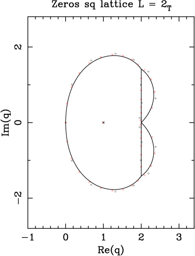
(((a)(a)	(((a)(b)
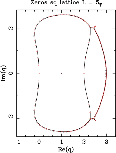
(((a)(c)	(((a)(d)

Figure 5: Limiting curves for square-lattice strips of width (a) $L=2$, (b) $L=3$, (c) $L=4$, and (d) $L=5$ with toroidal boundary conditions. We also show the zeros for the strips $L_{\text{F}}\times(5L)_{\text{P}}$ (black $\Box$) and $L_{\text{F}}\times(10L)_{\text{P}}$ (red $\circ$) for the same values of $L$.

In Figure 5(a) we have shown the chromatic zeros for the strips of lengths $n=10$ and $n=20$. We also show the limiting curve $\mathcal{B}_{2}$ where the chromatic zeros accumulate in the infinite-length limit.

The limiting curve $\mathcal{B}_{2}$ splits the complex $q$-plane into four regions. The regions inside the outer parts of $\mathcal{B}_{2}$ are characterized by a dominant eigenvalue belonging to the $\ell=1$ sector, while in the outer region the eigenvalue $\lambda_{0}$ dominates.

The curve $\mathcal{B}_{2}$ crosses the real $q$ axis at two points: $q=0$ and $q=2$. This latter point is in fact a multiple point. Finally, there is a single isolated limiting point at $q=1$.

3.2 $\bm{L=3}$

The chromatic polynomial for this strip was computed by Chang and Shrock [17] (in fact, they computed the full Potts-model partition function [19]).

The full transfer matrix ${\mathsf{T}}(3_{\text{T}})$ has dimension eight. In the basis $\{\delta_{1,1^{\prime}}\delta_{2,2^{\prime}}\delta_{3,3^{\prime}},\delta_{1,2^{\prime}}\delta_{2,1^{\prime}}+\ldots,\delta_{1,2^{\prime}}\delta_{3,3^{\prime}}+\ldots,\delta_{1,1^{\prime}}\delta_{2,2^{\prime}}+\ldots,\delta_{1,2^{\prime}}\delta_{1,2^{\prime}}+\ldots,\delta_{1,2^{\prime}}+\ldots,\delta_{1,1^{\prime}}+\ldots,1\}$ (where the dots “$\ldots$” mean all possible states equivalent under reflections and/or rotations), it takes the form

$${\mathsf{T}}(3_{\text{T}})\;=\;\left(\begin{array}[]{c|cccc|cc|c}-1&0&0&0&0&0&0&0\\ \hline\cr 0&s_{3}&0&0&-2&0&0&0\\ 0&0&s_{3}&-1&-1&0&0&0\\ 1&0&-2&s_{3}&0&0&0&0\\ 0&-1&-1&0&s_{3}&0&0&0\\ \hline\cr 0&-s_{4}&-s_{4}&1&7-2q&s_{3}-S&s_{3}&0\\ -1&0&-2s_{4}&-2s_{3}&2&2s_{3}&-S&0\\ \hline\cr 1&3s_{3}&6s_{3}&3s_{3}&6s_{3}&6S&3S&\lambda_{0}\\ \end{array}\right)$$ (3.3)

where we by vertical and horizontal lines show the lower-triangular block structure of this matrix, and

$$s_{k}&=q-k{}\\ S=q^{2}-5q+7{}\\ \lambda_{0}=q^{3}-6q^{2}+14q-13{}$$ (3.4)

The vectors $\bm{w}_{\text{id}}$ and $\bm{u}$ take the form

$$\bm{u}^{T}&=(A,0,0,3A,0,0,3A,A)\,,\qquad\text{with $A=q(q-1)(q-2)$}\\ \bm{w}_{\text{id}}^{T}=(1,0,0,0,0,0,0,0)$$ (3.5)

The eigenvalues can be obtained from the diagonal blocks $T_{\ell,\ell}$. Each block $T_{\ell,\ell}$ is characterized by the trivial bottom-row connectivity state $\mathcal{P}_{\text{bot}}=1$. We find the following eigenvalue structure for ${\mathsf{T}}(3_{\text{T}})$ (3.3):

• $\bm{\ell=0}$: There is a single eigenvalue $\lambda_{0}$ (LABEL:def_l0_Tsq3T) with amplitude $b^{(0)}=1$.

• $\bm{\ell=1}$: We find two eigenvalues: $\lambda_{1,1}=-(q^{2}-7q+13)$ with amplitude $b^{(1)}=q-1$ and $\lambda_{1,2}=-(q-2)^{2}$ with amplitude $2b^{(1)}=2(q-1)$.

• $\bm{\ell=2}$: The four eigenvalues are $\lambda_{2,1}=q-1$, $\lambda_{2,2}=q-2$, $\lambda_{2,3}=q-4$, and $\lambda_{2,4}=q-5$. The amplitudes are given respectively by $b^{(2)}_{2}$, $2b_{1}^{(2)}$, $2b^{(2)}_{2}$, and $b_{1}^{(2)}$ [c.f., (2.32)].

• $\bm{\ell=3}$: The eigenvalue is $\lambda_{3}=-1$ with amplitude $b^{(3)}$ (LABEL:def_b3).

In Figure 5(b) we have shown the chromatic zeros for the strips of lengths $n=15$ and $n=30$, as well as the limiting curve $\mathcal{B}_{3}$ where the chromatic zeros accumulate in the infinite-length limit. This curve splits the complex $q$-plane into three regions. The region containing the real segment $(0,2)$ is dominated by an eigenvalue from the $\ell=1$ sector. The region containing the real segment $(2,3)$ is dominated by the $\ell=2$ sector. The rest of the complex $q$-plane is dominated by the $\ell=0$ eigenvalue $\lambda_{0}$ (LABEL:def_l0_Tsq3T).

The curve $\mathcal{B}_{3}$ crosses the real $q$ axis at three points: $q=0$, $q=2$, and $q=3$. We also find a pair of complex conjugate T points at $q\approx 2.4692972375\pm 1.4013927796\,i$. Finally, there is a single isolated limiting point at $q=1$.

3.3 $\bm{L=4}$

The chromatic polynomial for this strip was computed by Chang and Shrock [16]. The full transfer matrix ${\mathsf{T}}(4_{\text{T}})$ has dimension $68$. In this case, we restrict ourselves to report the eigenvalue structure:

• $\bm{\ell=0}$: This block has dimension five with two sub-blocks of dimensions three and two. There are three distinct eigenvalues: $\lambda_{0,1}=(q-1)(q-3)$ and the solutions of a second-order equation [16, Eq. (2.12)]. All of them have the amplitude $b^{(0)}=1$.

• $\bm{\ell=1}$: This block has dimension $22$, and it contains three sub-blocks of dimensions six and eight (two of them). We find eight different eigenvalues. Two of them are the solutions of the second-order equation [16, Eq. (2.13)] with amplitudes $2b^{(1)}=2(q-1)$; The other six eigenvalues come from two distinct third-order equations [16, Eqs. (2.18)/(2.19)], with amplitudes $b^{(1)}=q-1$.

• $\bm{\ell=2}$: This block has dimension $33$ containing three sub-blocks of dimensions $8$, $12$, and $13$. Among these $33$ eigenvalues, we find $15$ distinct eigenvalues. Three of them are simple: $\lambda_{2,1}=q^{2}-5q+5$ with amplitude $b_{2}^{(2)}$, $\lambda_{2,2}=q^{2}-5q+7$ with amplitude $b_{1}^{(2)}$, and the special one $\lambda_{(2,3)}=2-q$ which also appears in the $\ell=3$ sector (see below). The next six eigenvalues are solutions of three second-order equations [16, Eqs. (2.14)–(2.16)], with amplitudes $b_{1}^{(2)}$, $2b_{1}^{(2)}$, and $b_{2}^{(2)}$, respectively [c.f., (2.32)]. The last six eigenvalues come from two third-order equations [16, Eqs. (2.20)/(2.21)], with amplitudes $b_{1}^{(2)}$ and $2b_{2}^{(2)}$, respectively.

• $\bm{\ell=2,3}$: The eigenvalue $\lambda_{(2,3)}=2-q$ appears in these two blocks with an amplitude $(q-2)(4q^{2}-13q-3)/6=b_{2}^{(2)}+2b_{2}^{(3)}$.

• $\bm{\ell=3}$: This block has dimension seven: in addition to $\lambda_{(2,3)}$, we find six other eigenvalues: $\lambda_{3,1}=5-q$ with amplitude $b_{1}^{(3)}$ [16, Eq. (2.8)]; $\lambda_{3,2}=4-q$ with amplitude $2b_{2}^{(3)}$ [16, Eq. (2.7)]; $\lambda_{3,3}=3-q$ with amplitude $2b_{1}^{(3)}$ [16, Eq. (2.6)]; $\lambda_{3,4}=1-q$ with amplitude $b_{1}^{(3)}$ [16, Eq. (2.4)]; and $\lambda_{3,5,\pm}=3-q\pm\sqrt{3}$ with common amplitude $2b_{2}^{(3)}$ [16, Eq. (2.17)].

• $\bm{\ell=4}$: This one-dimensional block gives $\lambda_{4}=1$ with amplitude $b^{(4)}$ (LABEL:def_b4).

Thus, for this strip we find $33$ different eigenvalues. All of them but $\lambda_{(2,3)}=2-q$, belong to a single $\ell$ sector.

In Figure 5(c) we have shown the chromatic zeros for the strips of lengths $n=20$ and $n=40$, as well as the limiting curve $\mathcal{B}_{4}$. This curve splits the complex $q$-plane into five regions. The region containing the real segment $(0,2)$ is dominated by an eigenvalue from the $\ell=1$ sector. The region containing the real segment $(2,q_{0}(4))$ with $q_{0}(4)\approx 2.7827657401$ is dominated by the $\ell=2$ sector. The rest of the complex $q$-plane (i.e., the other three regions) is dominated by the $\ell=0$ sector. Notice that the special eigenvalue $\lambda_{(2,3)}=q-2$ is not dominant in any open set of the complex $q$-plane.

The curve $\mathcal{B}_{4}$ crosses the real $q$ axis at three points: $q=0$, $q=2$, and $q=q_{0}(4)\approx 2.7827657401$. We also find three pairs of complex conjugate T points at $q\approx 2.4184666383\pm 1.7281014476\,i$, $q\approx 2.6228997762\pm 1.5279208067\,i$, $q\approx 2.7784542034\pm 0.9708262424\,i$. Finally, there is a single isolated limiting point at $q=1$.

3.4 $\bm{L=5}$

The full transfer matrix ${\mathsf{T}}(5_{\text{T}})$ has dimension $347$. The relevant eigenvalues can be extracted from the diagonal blocks $T_{\ell\ell}(5_{\text{T}})$. We find the following eigenvalue structure:

• $\bm{\ell=0}$: This block has dimension six. In the basis $\{\delta_{1^{\prime},3^{\prime}}+\ldots,\delta_{1^{\prime},3^{\prime}}\delta_{1,3}+\ldots,\delta_{1^{\prime},3^{\prime}}\delta_{1,4}+\ldots,\delta_{1^{\prime},3^{\prime}}\delta_{2,4}+\ldots,1,\delta_{1,3}+\ldots\}$ (where the dots “…” mean all equivalent states under rotations and reflections), it takes the form:

  $$T_{0,0}(5_{\text{T}})\;=\;\left(\begin{array}[]{cccc|cc}T_{1}&T_{2}&2T_{2}&2T_{2}&0&0\\ S-s_{3}&Ss_{2}&-2s_{2}s_{3}&2s_{3}&0&0\\ S-s_{3}&-s_{2}s_{3}&Ss_{2}+s_{3}&-s_{3}^{2}&0&0\\ S-s_{3}&s_{3}&-s_{3}^{2}&s_{2}(S-s_{3})&0&0\\ \hline\cr 0&0&0&0&T_{3}&S-s_{3}\\ 0&0&0&0&5T_{2}&T_{1}\end{array}\right)$$ (3.6)

  where $s_{k}$ and $S$ are defined in (LABEL:def_sk)/(LABEL:def_S), and

  $$T_{1}&=q^{5}-10q^{4}+45q^{3}-115q^{2}+169q-116\\ T_{2}=q^{4}-9q^{3}+34q^{2}-63q+47\\ T_{3}=q^{3}-9q^{2}+29q+32$$ (3.7)

  This matrix is block diagonal: the first four-dimensional block corresponds to the bottom-row connectivity $\mathcal{P}_{\text{bot}}=\delta_{1^{\prime},3^{\prime}}$, while the second two-dimensional block corresponds to the trivial bottom-row connectivity $\mathcal{P}_{\text{bot}}=1$.

  We find four distinct eigenvalues coming from two second-order equations:

  $$0&=\xi^{2}-\xi(2q^{3}-13q^{2}+28q-19)+q^{6}-13q^{5}+69q^{4}-191q^{3}\\ \quad+292q^{2}-236q+79{}\\ 0=\xi^{2}-\xi(q^{5}-10q^{4}+46q^{3}-124q^{2}+198q-148)+q^{8}-19q^{7}+159q^{6}\\ \quad-767q^{5}+2339q^{4}-4627q^{3}+5800q^{2}-4212q+1362{}$$ (3.8)

  Their amplitudes are $2b^{(0)}=2$ and $b^{(0)}=1$, respectively.

• $\bm{\ell=1}$: This block has dimension $67$ and it contains four sub-blocks of dimension $14$ (three of them) and $25$. We find $15$ different eigenvalues: $\lambda_{(1,2)}=-(q^{2}-4q+3)$ also appears in the $\ell=2$ block (see below), and the rest come from polynomial equations of order ten (with amplitude $2b^{(1)}=2(q-1)$) and four (with amplitude $b^{(1)}=q-1$).

• $\bm{\ell=1,2}$: The eigenvalue $\lambda_{(1,2)}=-(q^{2}-4q+3)$, appears in these two blocks with amplitude $(q+1)(q-2)/2=b^{(1)}+b_{1}^{(2)}$.

• $\bm{\ell=2}$: This block has dimension $190$ and it contains five sub-blocks of dimensions $31$, $33$ (three of them), and $60$. We find $36$ distinct eigenvalues, including $\lambda_{(1,2)}$. Two eigenvalues come from the second-order equation:

  $$\xi^{2}+\xi(2q^{2}-11q+16)+q^{4}-11q^{3}+44q^{2}-77q+51\;=\;0$$ (3.9)

  with amplitude $b^{(2)}_{2}$ (LABEL:def_b22). The other eigenvalues are the solutions of polynomial equations of order four, five, and twelve (two of them). Their amplitudes are are $b^{(2)}_{2}$, $b^{(2)}_{1}$, $2b^{(2)}_{1}$, and $2b^{(2)}_{2}$, respectively [c.f., (2.32)].

• $\bm{\ell=3}$: This block has dimension $72$, and it contains three sub-blocks of dimension $24$. The $24$ distinct eigenvalues come from polynomial equations of order three (two of them), six, and twelve. The corresponding amplitudes are $2b^{(3)}_{2}$, $b^{(3)}_{1}$, $2b^{(3)}_{1}$, and $2b^{(3)}_{2}$, respectively [c.f., (2.32)].

• $\bm{\ell=4}$: This block has dimension $11$. Three eigenvalues are rather simple: $\lambda_{4,1}=q-5$ with amplitude $b_{1}^{(4)}$; $\lambda_{4,2}=q-3$ with amplitude $2b_{2}^{(4)}$; and $\lambda_{4,3}=q-1$ with amplitude $b_{3}^{(4)}$ [c.f., (2.33)].. The next four are solutions of two second-order equations

  $$0&=\xi^{2}-\xi(2q-5)+q^{2}-5q+5\\ 0=\xi^{2}-\xi(2q-7)+q^{2}-7q+11$$ (3.10)

  with amplitudes $2b_{1}^{(4)}$ and $2b_{3}^{(4)}$, respectively. The last eigenvalues come from a fourth-order equation with amplitudes $2b_{2}^{(4)}$.

• $\bm{\ell=5}$: This one-dimensional block gives $\lambda_{5}=-1$ with amplitude $b^{(5)}$ (LABEL:def_b5).

For this strip we find $90$ different eigenvalues. All of them but one belong to a single $\ell$ sector. The only exception is the eigenvalue $\lambda_{(1,2)}=-(q^{2}-4q+3)$ which appears in the sectors $\ell=1,2$.

In Figure 5(d) we have shown the chromatic zeros for the strips of lengths $n=25$ and $n=50$, and the limiting curve $\mathcal{B}_{5}$. This curve splits the complex $q$-plane into three regions. The region containing the real segment $(0,2)$ is dominated by an eigenvalue from the $\ell=1$ sector. The region containing the real segment $(2,3)$ is dominated by the $\ell=2$ sector. The rest of the complex $q$-plane is dominated by the $\ell=0$ sector. Notice that the special eigenvalue $\lambda_{(1,2)}$ is not dominant in any open set of the complex $q$-plane.

The curve $\mathcal{B}_{5}$ crosses the real $q$ axis at three points: $q=0$, $q=2$, and $q=3$. We also find two pairs of complex conjugate T points at $q\approx 2.2834116867\pm 2.0404211832\,i$, $q\approx 2.4349888915\pm 1.9935503628\,i$. We also find a pair of complex-conjugate endpoints at $q\approx 2.5034648020\pm 2.0851731763\,i$. Finally, there is a single isolated limiting point at $q=1$.

3.5 $\bm{L=6}$

The full transfer matrix ${\mathsf{T}}(6_{\text{T}})$ has dimension $2789$. The relevant eigenvalues can be extracted from the diagonal blocks $T_{\ell\ell}(6_{\text{T}})$. We find the following eigenvalue structure:

• $\bm{\ell=0}$: This block has dimension 39, and it contains five sub-blocks of dimensions five, seven, eight (two of them), and eleven. We find eleven distinct eigenvalues. The simplest one is $\lambda_{0,1}=q^{4}-9q^{3}+30q^{2}-44q+25$ with amplitude $2b^{(0)}=2$. Two eigenvalues are the solutions of the second-order equation

  $$\xi^{2}-\xi(q^{4}-10q^{3}+39q^{2}-68q+38)-q^{7}+15q^{6}-93q^{5}+309q^{4}-598q^{3}+681q^{2}-422q+109\;=\;0$$ (3.11)

  with amplitude $b^{(0)}=1$. The other eigenvalues come from polynomial equations of order three (with amplitude $2b^{(0)}=2$) and five (with amplitude $b^{(0)}=1$).

• $\bm{\ell=1}$: This block has dimension $494$ and it contains eleven sub-blocks of dimensions ranging from $21$ to $71$. We find $48$ different eigenvalues in this block. The simplest ones are given by $\lambda_{(1,2)}=-(q^{3}-8q^{2}+20q-14)$ and $\lambda_{(1,2,3)}=-(q^{3}-6q^{2}+12q-8)$, which also they appear in other blocks (see below). Two eigenvalues are the solutions of the second-order equation:

  $$\xi^{2}+\xi(2q^{3}-16q^{2}+42q-38)+q^{6}-16q^{5}+104q^{4}-352q^{3}+656q^{2}-642q+262\;=\;0$$ (3.12)

  with amplitude $b^{(1)}=q-1$. The other eigenvalues come from polynomial equations of order ten, eleven (two of them), and twelve.

• $\bm{\ell=1,2}$: The eigenvalue $\lambda_{(1,2)}=-(q^{3}-8q^{2}+20q-14)$ appears in these two blocks with an amplitude $(q-2)(q+1)/2=b^{(1)}+b_{1}^{(2)}$.

• $\bm{\ell=2}$: This block has dimension $1432$ and it contains $13$ sub-blocks of dimensions between $56$ and $180$. We have found $120$ distinct eigenvalues: $\lambda_{(1,2)}$, $\lambda_{(1,2,3)}$, $\lambda_{(2,3)}=q^{2}-5q+5$ which also appears in the $\ell=3$ sector (see below), and $117$ eigenvalues coming from equations of order five (two equations), seven (two equations), nine, eleven, $13$, $14$ (two equations), and $16$ (two equations).

• $\bm{\ell=1,2,3}$: The eigenvalue $\lambda_{(1,2,3)}=-(q^{3}-6q^{2}+12q-8)$ appears in these three blocks with amplitude $(q-3)(2q^{2}-3q+4)/6=b^{(1)}+b_{1}^{(2)}+b_{1}^{(3)}$.

• $\bm{\ell=2,3}$: The eigenvalue $\lambda_{(2,3)}=q^{2}-5q+5$ appears in these two blocks with amplitude $(2q^{3}-9q^{2}+7q-6)/6=b_{1}^{(2)}+b_{1}^{(3)}$.

• $\bm{\ell=3}$: This block has dimension $644$ and it contains seven sub-blocks of dimensions between $31$ and $150$. We have found $82$ distinct eigenvalues coming from equations of order three, six, seven, eight (six equations), and nine (two equations). In addition, we obtain the already discussed eigenvalues $\lambda_{(1,2,3)}$ and $\lambda_{(2,3)}$.

• $\bm{\ell=4}$: This block has dimension $163$ and it contains four sub-blocks of dimensions $26$, $45$, and $46$ (two of them). We have found $49$ distinct eigenvalues. The simplest one is $\lambda_{4,1}=-(q-2)(q-3)$ with amplitude $b_{1}^{(4)}$ (LABEL:def_b41). Six eigenvalues are solutions of three second-order equations

  $$0&=\xi^{2}-\xi(2q^{2}-11q+13)+q^{4}-11q^{3}+43q^{2}-71q+40\\ 0=\xi^{2}-\xi(q^{2}-7q+8)-q^{3}+8q^{2}-18q+11\\ 0=\xi^{2}-\xi(q^{2}-7q+10)-q^{3}+8q^{2}-20q+15$$ (3.13)

  The other eigenvalues come from equations of order three (four equations), four (four equations), six, and eight.

• $\bm{\ell=5}$: This block has dimension $16$. The simplest eigenvalues are $\lambda_{5,1}=5-q$ (with amplitude $b_{1}^{(5)}$), $\lambda_{5,2}=4-q$ (with amplitude $2b_{1}^{(5)}$), $\lambda_{5,3}=2-q$ (with amplitude $2b_{1}^{(5)}$), and $\lambda_{5,4}=1-q$ (with amplitude $b_{1}^{(5)}$). Four eigenvalues are solutions of two second-order equations:

  $$0&=\xi^{2}+\xi(2q-7)+q^{2}-7q+11\\ 0=\xi^{2}+\xi(2q-5)+q^{2}-5q+5$$ (3.14)

  The remaining eight eigenvalues come from two fourth-order equations. The amplitude of all these twelve eigenvalues is $2b_{2}^{(5)}$ (LABEL:def_b52).

• $\bm{\ell=6}$: This one-dimensional block gives $\lambda_{6}=1$ with amplitude $b^{(6)}$ (LABEL:def_b6).

For this strip we find $325$ different eigenvalues; all of them but three ($\lambda_{(1,2)}$, $\lambda_{(1,2,3)}$, and $\lambda_{(2,3)}$) belong to a single $\ell$ sector.

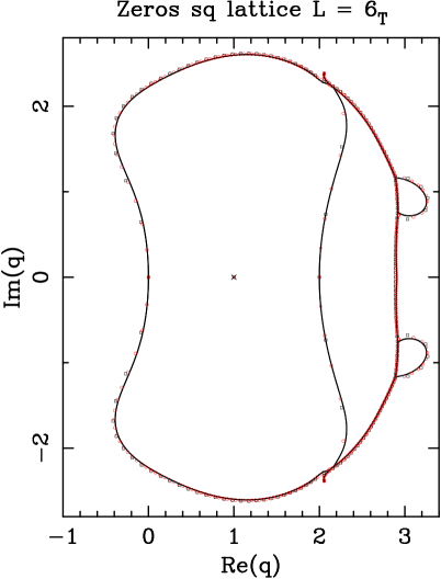
(((a)(a)	(((a)(b)

Figure 6: Limiting curves for square-lattice strips of width (a) $L=6$, and (b) $L=7$ with toroidal boundary conditions. We also show the zeros for the strips $L_{\text{F}}\times(5L)_{\text{P}}$ (black $\Box$) and $L_{\text{F}}\times(10L)_{\text{P}}$ (red $\circ$) for the same values of $L$.

In Figure 6(a) we have shown the chromatic zeros for the strips of lengths $n=30$ and $n=60$, and the limiting curve $\mathcal{B}_{6}$. This curve splits the complex $q$-plane into four regions. The region containing the real segment $(0,2)$ is dominated by an eigenvalue from the $\ell=1$ sector. The region containing the real segment $(2,5/2)$ is dominated by the $\ell=2$ sector. The two small complex conjugate regions are dominated by the $\ell=1$ sector. The rest of the complex $q$-plane is dominated by the $\ell=0$ sector.

The curve $\mathcal{B}_{5}$ crosses the real $q$ axis at three points: $q=0$, $q=2$, and $q\approx 2.9078023424$. We also find four pairs of complex conjugate T points at $q\approx 2.1180081660\pm 2.2566257839\,i$, $q\approx 2.1632612447\pm 2.2209172289\,i$, $q\approx 2.8895175995\pm 1.1648906031\,i$, and $q\approx 2.9197649745\pm 0.7583704656\,i$. We also find a pair of complex-conjugate endpoints at $q\approx 2.0571168133\pm 2.3885607275\,i$. Finally, there is a single isolated limiting point at $q=1$.

3.6 $\bm{L=7}$

The full transfer matrix ${\mathsf{T}}(7_{\text{T}})$ has dimension $20766$. We have been unable to obtain the full eigenvalue structure, as some of the blocks for $\ell=2,3$ are very large. Thus, we cannot obtain the amplitudes. We find the following (partial) eigenvalue structure:

• $\bm{\ell=0}$: This block has dimension $111$, and it contains six sub-blocks of dimensions six and $21$ (five of them). We find $21$ different eigenvalues coming from polynomial equations of order six and $15$.

• $\bm{\ell=1}$: This block has dimension $2794$, and it contains $19$ sub-blocks of dimensions $103$ and $196$. We find $112$ different eigenvalues coming from polynomial equations of order nine, $19$, and $84$.

• $\bm{\ell=2}$: This block has dimension $10224$, and it contains $26$ sub-blocks of dimensions $270$, $276$, and $532$. We find $292$ different eigenvalues coming from polynomial equations of order $16$, $22$, $26$, and $114$ (two of them) arising from the characteristic polynomials of the sub-blocks of dimensions $\leq 276$. This description is not complete, as we cannot obtain the characteristic polynomial of the sub-blocks of dimension $532$. However, we can numerically diagonalize this sub-block and find that it provides $12$ additional distinct eigenvalues; hence, we expect to have $304$ distinct eigenvalues in this sector.

• $\bm{\ell=3}$: This block has dimension $5615$, and it contains $17$ sub-blocks of dimensions $247$ and $483$. We find $247$ different eigenvalues coming from the polynomial equations of order $17$, $23$, $69$, and $138$ that arise from the characteristic polynomials of the smaller sub-blocks. Furthermore, we numerically find that the larger sub-blocks of dimension $483$ contains only six additional distinct eigenvalues. Thus, we expect $253$ distinct eigenvalues for this sector.

• $\bm{\ell=4}$: This block has dimension $2711$, and it contains eight sub-blocks of dimensions $155$, $158$, and $308$. We find $165$ different eigenvalues coming from polynomial equations of order three, four, seven, eight, eleven, $33$ (two of them), and $66$.

• $\bm{\ell=5}$: This block has dimension $288$, and it contains four sub-blocks of dimension $72$. We find $72$ different eigenvalues coming from polynomial equations of order four, eight, twelve, and $48$.

• $\bm{\ell=6}$: This block has dimension $22$. We find four simple eigenvalues $\lambda_{6,1}=q-5$, $\lambda_{6,2}=q-4$, $\lambda_{6,3}=q-2$, and $\lambda_{6,4}=q-1$. The other come from equations of order three and six (two of each).

• $\bm{\ell=7}$: This one-dimensional block gives $\lambda_{7}=-1$.

In Figure 6(b) we have shown the chromatic zeros for the strips of lengths $n=35$ and $n=70$, and the limiting curve $\mathcal{B}_{7}$.

The curve $\mathcal{B}_{7}$ crosses the real $q$ axis at three points: $q=0$, $q=2$, and $q=3$. We also find six pairs of complex conjugate T points at $q\approx 1.4876491726\pm 2.5577806355\,i$, $q\approx 1.6498030004\pm 2.5002880707\,i$, $q\approx 1.9765852319\pm 2.3664338035\,i$, $q\approx 2.5531414480\pm 1.8775702667\,i$, $q\approx 2.8395564367\pm 1.4513813377\,i$, and $q\approx 2.8734078918\pm 1.3454749268\,i$. There are two complex conjugate oval-shaped regions between the T points at $q\approx 1.488\pm 2.558\,i$ and $q\approx 1.650\pm 2.500\,i$. And there is another pair of small bulb-like regions between the T points at $q\approx 2.840\pm 1.451\,i$ and $q\approx 2.873\pm 1.345\,i$.

Thus, the limiting curve $\mathcal{B}_{7}$ splits the complex $q$-plane into seven regions. The region containing the real segment $(0,2)$ is dominated by an eigenvalue from the $\ell=1$ sector. The region containing the real segment $(2,3)$ is dominated by the $\ell=2$ sector. The two small complex conjugate oval-shaped regions are dominated by the $\ell=0$ sector; and the two small complex conjugate bulb-like regions are dominated by the $\ell=1$ sector. The rest of the complex $q$-plane is dominated by the $\ell=0$ sector.

We also find a pair of complex-conjugate endpoints at $q\approx 1.6947007027\pm 2.5327609879\,i$. Finally, there is a single isolated limiting point at $q=1$.

4 Triangular-lattice numerical results

In this section we will analyze the results for the triangular-lattice strips of widths $2\leq L\leq 7$. We have checked our results using (in addition to the already known cases $L\leq 4$ [16, 18, 19]) the identity (2.22).

As for the square lattice, for each $L$ we give a detailed description of the eigenvalues and amplitudes. For the already known cases $L=2,3$, we include for the sake of clarity the full expressions for the transfer matrices and the left and right vectors. The exact expressions for the new cases $L=5,6$ can be found in the mathematica file transfer6_triT.m available as part of the on-line version of this paper in the cond-mat archive at arXiv.org. As in the square-lattice case, for $L=7$ we can only present a partial description of the eigenvalue structure, as some of the sub-blocks are very large.

4.1 $\bm{L=2}$

The chromatic polynomial for this strip was computed by Chang and Shrock [19] (in fact, they computed the full Potts-model partition function).

The full transfer matrix ${\mathsf{T}}(2_{\text{T}})$ has dimension five. In the basis $\{\delta_{1^{\prime},2}\delta_{2^{\prime},1},\delta_{1^{\prime},1}\delta_{2,2^{\prime}},\delta_{1^{\prime},2}+\delta_{2^{\prime},1},\delta_{1^{\prime},1}+\delta_{2^{\prime},2},1\}$, we find the following transfer matrix with a lower-triangular block structure

$${\mathsf{T}}(2_{\text{T}})\;=\;\left(\begin{array}[]{cc|cc|c}1&1&0&0&0\\ 1&1&0&0&0\\ \hline\cr-1&-1&3-q&3-q&0\\ -1&-1&3-q&3-q&0\\ \hline\cr 1&1&2(q-3)&2(q-3)&q^{2}-5q+6\end{array}\right)$$ (4.1)

The right $\bm{w}_{\text{id}}$ and left $\bm{u}$ vectors are given by

$$\bm{u}^{T}&=(0,A,0,2A,A)\,,\qquad\text{with $A=q(q-1)$}\\ \bm{w}_{\text{id}}^{T}=(0,1,0,0,0)$$ (4.2)

The eigenvalues can be obtained from the diagonal blocks $T_{\ell,\ell}$. (each of them associated to $\mathcal{P}_{\text{bot}}=1$).

After some algebra, we find the following eigenvalues and amplitudes:

• $\bm{\ell=0}$: The eigenvalue is $\lambda_{0}=q^{2}-5q+6$ with amplitude $b^{(0)}=1$.

• $\bm{\ell=1}$: There are two eigenvalues: $\lambda_{1}=-2(q-3)$ with amplitude $b^{(1)}=q-1$, and $\lambda_{\odot}=0$, which is common to the $\ell=2$ block.

• $\bm{\ell=1,2}$: The eigenvalue $\lambda_{\odot}=0$ appears in these two blocks. Its amplitude is irrelevant for the computation of both the limiting curve $\mathcal{B}_{2}$ and the chromatic polynomials $P_{2_{\text{P}}\times n_{\text{P}}}(q)$.

• $\bm{\ell=2}$: We find $\lambda_{\odot}=0$, and the eigenvalue $\lambda_{2}=2$ with amplitude $b_{1}^{(2)}$ (LABEL:def_b21).

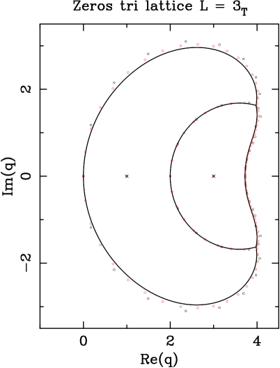
(((a)(a)	(((a)(b)
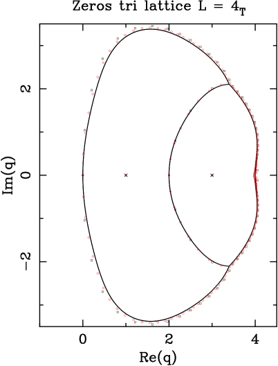
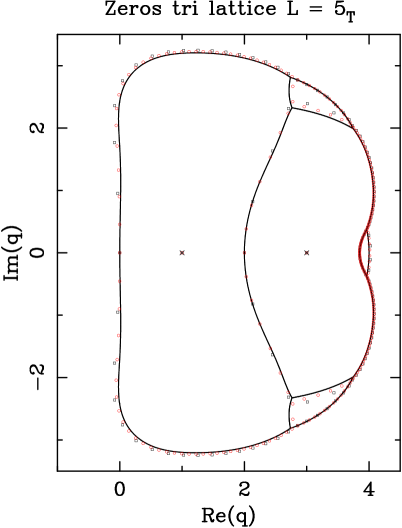
(((a)(c)	(((a)(d)

Figure 7: Limiting curves for triangular-lattice strips of width (a) $L=2$, (b) $L=3$, (c) $L=4$, and (d) $L=5$ with toroidal boundary conditions. We also show the zeros for the strips $L_{\text{F}}\times(5L)_{\text{P}}$ (black $\Box$) and $L_{\text{F}}\times(10L)_{\text{P}}$ (red $\circ$) for the same values of $L$.

In Figure 7(a) we have shown the chromatic zeros for the strips of lengths $n=10$ and $n=20$, and the limiting curve $\mathcal{B}_{2}$. This curve splits the complex $q$-plane into three regions. The outer one is dominated by the $\ell=0$ sector. The one containing the real interval $q\in(0,2)$ is dominated by the $\ell=1$ sector; and the one containing the real interval $q\in(2,4)$ is dominated by the $\ell=2$ sector.

The curve $\mathcal{B}_{2}$ crosses the real $q$ axis at three points: $q=0$, $q=2$, and $q=4$. This latter point is in fact a multiple point. Finally, there are two isolated limiting points at $q=1$ and $q=3$.

4.2 $\bm{L=3}$

The chromatic polynomial for this strip was first computed by Chang and Shrock [18]. The full transfer matrix ${\mathsf{T}}(3_{\text{T}})$ has dimension $13$. In the basis $\{\delta_{1,3^{\prime}}\delta_{2,1^{\prime}}\delta_{3,2^{\prime}},\delta_{1,2^{\prime}}\delta_{2,3^{\prime}}\delta_{3,1^{\prime}},$ $\delta_{1,1^{\prime}}\delta_{2,2^{\prime}}\delta_{3,3^{\prime}},\delta_{1,2^{\prime}}\delta_{2,1^{\prime}}+\ldots,\delta_{1,2^{\prime}}\delta_{3,1^{\prime}}+\ldots,\delta_{1,1^{\prime}}\delta_{2,2^{\prime}}+\ldots,\delta_{2,1^{\prime}}\delta_{3,2^{\prime}}+\ldots,\delta_{2,1^{\prime}}\delta_{3,3^{\prime}}+\ldots,\delta_{1,2^{\prime}}\delta_{3,3^{\prime}}+\ldots,\delta_{1,2^{\prime}}+\ldots,\delta_{1,1^{\prime}}+\ldots,\delta_{1,3^{\prime}}+\ldots,1\}$ (where the dots “…” mean all possible connectivity states symmetric under rotations), it takes the form

$${\mathsf{T}}(3_{\text{T}})\;=\;\left(\begin{array}[]{ccc|cccccc|ccc|c}-1&0&-1&0&0&0&0&0&0&0&0&0&0\\ -1&-1&0&0&0&0&0&0&0&0&0&0&0\\ 0&-1&-1&0&0&0&0&0&0&0&0&0&0\\ \hline\cr 1&0&0&s_{4}&-1&-1&s_{4}&s_{4}&0&0&0&0&0\\ 1&1&0&s_{4}&s_{4}&0&s_{4}&-1&-1&0&0&0&0\\ 0&1&1&-1&s_{4}&s_{4}&0&-1&s_{4}&0&0&0&0\\ 1&0&1&-1&0&s_{4}&s_{4}&s_{4}&-1&0&0&0&0\\ 0&0&1&0&-1&s_{4}&-1&s_{4}&s_{4}&0&0&0&0\\ 0&1&0&s_{4}&s_{4}&-1&-1&0&s_{4}&0&0&0&0\\ \hline\cr-1&-1&0&-2s_{4}&-2s_{4}&2&-2s_{4}&-s_{5}&-s_{5}&-R&2s_{3}&-R&0\\ 0&-1&-1&-s_{5}&-2s_{4}&-2s_{4}&2&-s_{5}&-2s_{4}&-R&-R&2s_{3}&0\\ -1&0&-1&-s_{5}&2&-2s_{4}&-2s_{4}&-2s_{4}&-s_{5}&2s_{3}&-R&-R&0\\ \hline\cr 1&1&1&3s_{4}&3s_{4}&3_{s}4&3s_{4}&3s_{4}&3s_{4}&3R&3R&3R&\lambda_{0}\end{array}\right)$$ (4.3)

where $s_{k}$ is defined in (LABEL:def_sk) and

$$R&=q^{2}-7q+13{}\\ \lambda_{0}=q^{3}-9q^{2}+29q-32{}$$ (4.4)

The right $\bm{w}_{\text{id}}$ and left $\bm{u}$ vectors are given by

$$\bm{u}^{T}&=(0,0,A,0,0,3A,0,0,0,0,3A,0A)\,,\qquad\text{with $A=q(q-1)(q-2)$}\\ \bm{w}_{\text{id}}^{T}=(0,0,1,0,0,0,0,0,0,0,0,0,0)$$ (4.5)

The eigenvalues can be obtained from the diagonal blocks $T_{\ell,\ell}$. (each of them associated to $\mathcal{P}_{\text{bot}}=1$). We find the following eigenvalue structure:

• $\bm{\ell=0}$: There is a single eigenvalue $\lambda_{0}=q^{3}-9q^{2}+29q-32$ with amplitude $b^{(0)}=1$.

• $\bm{\ell=1}$: There are three distinct eigenvalues $\lambda_{1,1}=-2(q-4)^{2}$, and $\lambda_{1,2\pm}=(q^{2}-5q+7)\,e^{\pm 2\pi i/3}$, with amplitude $b^{(1)}=q-1$.

• $\bm{\ell=2}$: The eigenvalues $\lambda_{(2,3\pm)}=e^{\pm 2\pi i/3}$ also appear in the $\ell=3$ (see below). We also find $\lambda_{2,1}=q-2$, $\lambda_{2,2}=3q-14$, and $\lambda_{2,3\pm}=(7-2q)e^{\pm 2\pi i/3}$. The corresponding amplitudes are $b^{(2)}_{2}$, $b_{1}^{(2)}$, and $b^{(2)}_{2}$, respectively [c.f., (2.32)].

• $\bm{\ell=2,3}$: The complex-conjugate pair $\lambda_{(2,3\pm)}=e^{\pm 2\pi i/3}$ appears in these two blocks with an amplitude $q(q-1)(2q-7)/6=b_{1}^{(2)}+b_{2}^{(3)}=b_{2}^{(2)}+b_{1}^{(3)}$. Please note that in this case the linear combination for the amplitude is not unambiguously determined.

• $\bm{\ell=3}$: In addition to $\lambda_{(2,3\pm)}$, we find $\lambda_{3}=-2$ with amplitude $b_{1}^{(3)}$ (LABEL:def_b31).

In Figure 7(b) we have shown the chromatic zeros for the strips of lengths $n=15$ and $n=30$, and the limiting curve $\mathcal{B}_{3}$. This curve splits the complex $q$-plane into three regions. The region containing the real segment $(0,2)$ is dominated by an eigenvalue from the $\ell=1$ sector. The region containing the real segment $(2,3]$ is dominated by the $\ell=2$ sector. The rest of the complex $q$-plane is dominated by the $\ell=0$ eigenvalue $\lambda_{0}$ (LABEL:def_l0_Ttri3T).

The curve $\mathcal{B}_{3}$ crosses the real $q$ axis at three points: $q=0$, $q=2$, and $q\approx 3.7240755514$. We also find a pair of complex conjugate T points at $q\approx 3.9777108575\pm 1.6284204463\,i$. Finally, there are two isolated limiting points at $q=1,3$.

4.3 $\bm{L=4}$

The chromatic polynomial for this strip was computed by Chang and Shrock [16]. The full transfer matrix ${\mathsf{T}}(4_{\text{T}})$ has dimension $99$. In this case, we restrict ourselves to report the eigenvalue structure:

• $\bm{\ell\geq 0}$: The eigenvalue $\lambda_{\odot}=0$ is common to all blocks $0\leq\ell\leq 4$. Its amplitude cannot be computed from our analysis; but it is unimportant to compute the chromatic polynomials and the limiting curve.

• $\bm{\ell=0}$: This block has dimension five with two sub-blocks of dimensions three and two. In addition to $\lambda_{\odot}=0$, we find two distinct eigenvalues coming from a second-order equation [16, Eq. (4.9)] and with amplitude $b^{(0)}=1$.

• $\bm{\ell=1}$: This block has dimension $26$, and it contains three sub-blocks of dimensions six, and ten (two of them). We find eight different eigenvalues, one of them being $\lambda_{\odot}=0$. The other eigenvalues come from a third-order equation [16, Eq. (4.12)] and from a fourth-order equation [16, Eq. (4.14)]. The amplitudes are in all cases $b^{(1)}=q-1$.

• $\bm{\ell=2}$: This block has dimension $52$, and it contains three sub-blocks of dimensions $12$, and $20$ (two of them). There are $18$ different eigenvalues. In addition to $\lambda_{\odot}=0$, we find two simple ones: $\lambda_{2,1}=2(3-q)$ and $\lambda_{2,2}=2(q-3)^{2}$, both with amplitudes $b_{2}^{(2)}$. The other eigenvalues come from polynomial equations of order two, three, four, and six, respectively [16, Eqs. (4.11)/(4.13)/(4.15)/(4.17)]. The corresponding amplitudes are $b_{1}^{(2)}$ for the first three, and $b_{2}^{(2)}$ for the last one [c.f. (2.32)].

• $\bm{\ell=3}$: This block has dimension $12$. We find three simple eigenvalues, $\lambda_{\odot}=0$, $\lambda_{3,1}=3-q$ with amplitude $2b_{2}^{(3)}$, and $\lambda_{3,2}=2(9-2q)$ with amplitude $b_{1}^{(3)}$ (LABEL:def_b31). We also find six eigenvalues coming from polynomial equations of order two [16, Eq. (4.10)] and six [16, Eq. (4.16)], with common amplitude $b_{2}^{(3)}$. The remaining two eigenvalues $\lambda_{(3,4\pm)}$ are common to the $\ell=4$ block (see below).

• $\bm{\ell=3,4}$: There are two eigenvalues common to the $\ell=3,4$ sectors: $\lambda_{(3,4\pm)}=1\pm i$ with amplitude $(q-1)(q-2)(3q^{2}-11q-6)/12=b_{1}^{(3)}+b_{2}^{(4)}$.

• $\bm{\ell=4}$: This is a four-dimensional block. In addition to $\lambda_{\odot}=0$ and $\lambda_{(3,4\pm)}$, we find $\lambda_{4}=2$ with amplitude $b_{1}^{(4)}$ (LABEL:def_b41).

Thus, for this strip we find $38$ distinct eigenvalues. All of them but three ($\lambda_{\odot}$ and $\lambda_{(3,4\pm)}$) belong to a single $\ell$ sector.

In Figure 7(c) we have shown the chromatic zeros for the strips of lengths $n=20$ and $n=40$, and the limiting curve $\mathcal{B}_{4}$. This curve splits the complex $q$-plane into three regions. The region containing the real segment $(0,2)$ is dominated by an eigenvalue from the $\ell=1$ sector. The region containing the real segment $(2,4)$ is dominated by the $\ell=2$ sector. The rest of the complex $q$-plane is dominated by the $\ell=0$ sector.

The curve $\mathcal{B}_{4}$ crosses the real $q$ axis at three points: $q=0$, $q=2$, and $q=4$. We also find a pair of complex conjugate T points at $q\approx 3.3943280448\pm 2.1041744504\,i$. Finally, there are two isolated limiting points at $q=1,3$.

4.4 $\bm{L=5}$

The full transfer matrix ${\mathsf{T}}(5_{\text{T}})$ has dimension $653$. The relevant eigenvalues can be extracted from the diagonal blocks $T_{\ell\ell}(5_{\text{T}})$. We find the following eigenvalue structure:

• $\bm{\ell=0}$: This block has dimension eight, and it contains two sub-blocks of dimensions two and six. We find six distinct eigenvalues (with amplitude $b^{(0)}=1$) coming from a fourth-order equation and the following second-order equation:

  $$0 = \xi^{2}-\xi(q^{5}-15q^{4}+98q^{3}-355q^{2}+711q-614)+3q^{8}-75q^{7}+817q^{6}$$ (4.6)

  $$-5062q^{5}+19492q^{4}-47696q^{3}+72273q^{2}-61822q+22764$$

• $\bm{\ell=1}$: This block has dimension $125$ and it contains seven sub-blocks of dimension $25$. We find $24$ different eigenvalues in this block. The eigenvalue $\lambda_{(1,2)}=-(q^{2}-5q+6)$ also appears in the $\ell=2$ block (see below). The other eigenvalues come from polynomial equations of order three and $20$. They all have the same amplitude $b^{(1)}=q-1$.

• $\bm{\ell=1,2}$: The eigenvalue $\lambda_{(1,2)}=-(q^{2}-5q+6)$ with amplitude $2q(q-2)=2(b^{(1)}+b_{1}^{(2)}+b_{2}^{(2)})$ appears in these two blocks.

• $\bm{\ell=2}$: This block has dimension $360$ and it contains six sub-blocks of dimension $60$. We find $57$ distinct eigenvalues, including $\lambda_{(1,2)}$. We also find the simple eigenvalue $\lambda_{2,1}=-(q-4)(2q-7)$ with amplitude $b_{2}^{(2)}$ (LABEL:def_b22). The other eigenvalues come from polynomial equations of order three, four, and $24$ (two of them).

• $\bm{\ell=3}$: This block has dimension $135$ and it contains three sub-blocks of dimension $45$. The $42$ distinct eigenvalues come from the solutions of polynomial equations of order: three (two of them), $12$, and $24$.

• $\bm{\ell=4}$: This block has dimension $20$. Three eigenvalues are rather simple: $\lambda_{4,1}=q-4$ with amplitude $2b_{2}^{(4)}$, $\lambda_{4,2}=q-2$ with amplitude $b_{3}^{(4)}$, and $\lambda_{4,3}=5q-22$ with amplitude $b_{1}^{(4)}$. Four eigenvalues $\lambda_{(4,5,i)}$ are common to the $\ell=5$ block (see below). The other eigenvalues come from polynomial equations of order four and eight, with amplitudes $b_{3}^{(4)}$ and $b_{2}^{(4)}$, respectively [c.f., (2.33)].

• $\bm{\ell=4,5}$: The four eigenvalues $\lambda_{(4,5,i)}$ are the solution of the equation

  $$\xi^{4}+3\xi^{3}+4\xi^{2}+2\xi+1\;=\;0$$ (4.7)

  Their amplitude is $q(q-3)(q-2)(4q^{2}-15q+1)/20=b_{1}^{(4)}+b_{2}^{(5)}=b_{3}^{(4)}+b_{1}^{(5)}$. Again, we find an ambiguity in the linear combination of basic amplitudes.

• $\bm{\ell=5}$: This block is five-dimensional. In addition to $\lambda_{(4,5,i)}$, we find $\lambda_{5}=-2$ with amplitude $b_{1}^{(5)}$ (LABEL:def_b51).

Thus, for this strip we find $148$ different eigenvalues. All of them but five ($\lambda_{(1,2)}=-(q^{2}-5q+6)$ and $\lambda_{(4,5,i)}$) belong to a single $\ell$ sector.

In Figure 7(d) we have shown the chromatic zeros for the strips of lengths $n=25$ and $n=50$, and the limiting curve $\mathcal{B}_{5}$. This curve splits the complex $q$-plane into six regions. The region containing the real segment $(0,2)$ is dominated by an eigenvalue from the $\ell=1$ sector. The regions containing the real segment $(2,4)$ is dominated by the $\ell=2$ sector. The rest of the complex $q$-plane (including the two complex-conjugate triangular-shaped regions) is dominated by the $\ell=0$ sector.

The curve $\mathcal{B}_{5}$ crosses the real $q$ axis at four points: $q=0$, $q=2$, $q\approx 3.8482632901$ and $q=4$. We also find four pairs of complex conjugate T points at $q\approx 2.7382976052\pm 2.8142366786\,i$, $q\approx 2.7643522733\pm 2.3252257137\,i$, $q\approx 3.7492171129\pm 1.9879721106\,i$, and $q\approx 3.9634199872\pm 0.3751435740\,i$. Finally, there are two isolated limiting points at $q=1,3$.

4.5 $\bm{L=6}$

The full transfer matrix ${\mathsf{T}}(6_{\text{T}})$ has dimension $5194$. The relevant eigenvalues can be extracted from the diagonal blocks $T_{\ell\ell}(6_{\text{T}})$.

• $\bm{\ell\geq 0}$: There is a single eigenvalue common to all blocks $\lambda_{\odot}=0$. As for the cases $L=2,4$, its amplitude cannot be determined; but it is irrelevant to compute both the chromatic polynomials and the limiting curve.

• $\bm{\ell=0}$: This block has dimension $49$, and it contains five sub-blocks of dimensions ranging from five to $15$. We find $14$ distinct eigenvalues: $\lambda_{\odot}=0$, the solutions of the second-order equation

  $$0 = \xi^{2}-\xi(3q^{4}-33q^{3}+132q^{2}-225q+135)+3q^{8}-66q^{7}+627q^{6}$$ (4.8)

  $$-3354q^{5}+11028q^{4}-22770q^{3}+28755q^{2}-20250q+6075$$

  and the solutions of equations of order five and six. All these eigenvalues have the amplitude $b^{(0)}=1$.

• $\bm{\ell=1}$: This block has dimension $843$ and it contains $13$ sub-blocks of dimensions ranging from $25$ to $71$. We find $62$ different eigenvalues in this block: $\lambda_{\odot}=0$, the solutions of the second-order equation

  $$\xi^{2}+\xi(3q^{3}-27q^{2}+79q-75)+q^{6}-18q^{5}+131q^{4}-492q^{3}+1000q^{2}-1032q+414=0$$ (4.9)

  and the solutions of equations of order four, nine, $22$, and $24$.

• $\bm{\ell=2}$: This block has dimension $2712$ and it contains $21$ sub-blocks of dimensions ranging from $96$ to $180$. We find $165$ different eigenvalues in this block: $\lambda_{\odot}=0$, and the solutions of polynomial equations of order three (two of them), four (two of them), ten (three of them), $28$ (two of them), and $32$ (two of them).

• $\bm{\ell=3}$: This block has dimension $1254$ and it contains nine sub-blocks of dimensions ranging from $54$ to $150$. We find $136$ different eigenvalues in this block: $\lambda_{\odot}=0$, $\lambda_{3,1}=(q-2)(q-3)$ with amplitude $5b_{1}^{(3)}$, and solutions of equations of order four, six, eight, $16$ (five of them), and $18$ (two of them).

• $\bm{\ell=4}$: This block has dimension $300$ and it contains five sub-blocks of dimensions ranging from $48$ to $84$. We find $76$ different eigenvalues in this block: $\lambda_{\odot}=0$, $\lambda_{4,1}=3q^{2}-18q+26$ with amplitude $b_{3}^{(4)}$ (LABEL:def_b43), $\lambda_{4,2}=2(3-q)$ with amplitude $3b_{3}^{(4)}$, the solutions of the second-order equation

  $$\xi^{2}+4q^{4}-44q^{3}+176q^{2}-304q+192\;=\;0$$ (4.10)

  with amplitude $b_{1}^{(4)}$, and the solutions of equations of order three, four, six (two of them), eight (three of them), twelve, and $16$.

• $\bm{\ell=5}$: This block has dimension $30$, and it contains $28$ different eigenvalues: $\lambda_{\odot}=0$, $\lambda_{5,1}=26-6q$ with amplitude $b_{1}^{(5)}$ (LABEL:def_b51), the solutions of the second-order equation

  $$\xi^{2}+\xi(2q-7)+q^{2}-7q+11\;=\;0$$ (4.11)

  with amplitude $2b_{2}^{(5)}$, four eigenvalues $\lambda_{(5,6,i)}$ common to the $\ell=6$ sector (see below), and the solutions of equations of order four and eight (two of them).

• $\bm{\ell=5,6}$: There are four common non-zero eigenvalues to these two sectors, coming from two second-order equations: $\lambda_{(5,6,1\pm)}=\sqrt{3}\,e^{\pm i\pi/6}$ with amplitude $(q-3)(5q^{5}-39q^{4}+93q^{3}-76q^{2}+22q+10)$, and $\lambda_{(5,6,2\pm)}=e^{\pm i\pi/3}$ with amplitude $(q-1)(5q^{5}-49q^{4}+161q^{3}-184q^{2}+6q+30)$.

• $\bm{\ell=6}$: This block has dimension $6$. The eigenvalues are $\lambda_{\odot}=0$, $\lambda_{(5,6,i)}$, and $\lambda_{6}=2$ with amplitude $q(q-3)(q-1)(q^{3}-8q+19q-11)/6$.

Thus, in this strip we find $476$ distinct eigenvalues. All of them but five ($\lambda_{\odot}=0$ and $\lambda_{(5,6,i)}$) belong to a single sector.

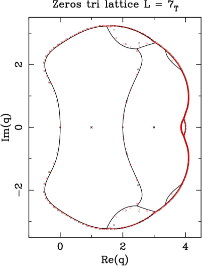
(((a)(a)	(((a)(b)

Figure 8: Limiting curves for triangular-lattice strips of width (a) $L=6$, and (b) $L=7$ with toroidal boundary conditions. We also show the zeros for the strips $L_{\text{F}}\times(5L)_{\text{P}}$ (black $\Box$) and $L_{\text{F}}\times(10L)_{\text{P}}$ (red $\circ$) for the same values of $L$.

In Figure 8(a) we have shown the chromatic zeros for the strips of lengths $n=30$ and $n=60$, and the limiting curve $\mathcal{B}_{6}$. This curve splits the complex $q$-plane into seven regions. The region containing the real segment $(0,2)$ is dominated by an eigenvalue from the $\ell=1$ sector. The region containing the real segment $(2,3)$ is dominated by the $\ell=2$ sector. The two bulb-like complex-conjugate regions appearing on the right hand-side of the limiting curve belong to the $\ell=1$ sector and they are rather special (see below). The rest of the complex $q$-plane (including the two complex-conjugate triangular-shaped regions) is dominated by the $\ell=0$ sector.

The curve $\mathcal{B}_{6}$ crosses the real $q$ axis at three points: $q=0$, $q=2$, and $q\approx 3.7943886378$. We also find five pairs of complex conjugate T points at $q\approx 2.0352758561\pm 3.1492288108\,i$, $q\approx 3.3399899103\pm 2.4428522934\,i$, $q\approx 2.5037195029\pm 2.3940503612\,i$, $q\approx 4.1131475777\pm 0.7636584371\,i$, and $q\approx 4.1295836790\pm 0.8010545279\,i$. Finally, there are two isolated limiting points at $q=1,3$.

Important technical remark. As stated above, the two bulb-like complex-conjugate protruding from T points $q\approx 4.11\pm 0.76\,i$ and $q\approx 4.13\pm 0.80\,i$, are rather special. Their peculiarity arises from the fact that inside these two bulb-like regions there is a pair of exactly equimodular dominant eigenvalues [with non-zero amplitudes $\sim(q-1)$]. Indeed, we do not see chromatic zeros becoming dense in the interior of these regions, but only on their boundaries.

The explanation of this phenomenon is rather simple: the two dominant eigenvalues come from a polynomial equation of order $24$ belonging to the $\ell=1$ sector. A closer look at this equation reveals that its roots $z_{k}$ can be written as $z_{k}=z_{0,k}e^{\pm\pi i/3}$ where the $z_{0,k}$ are the roots of another polynomial equation of order $12$ with integer coefficients (that can be easily computed). It is important to stress that the existence of this pair of equimodular eigenvalues does not mean that the chromatic zeros accumulate in this open set in the infinite-length limit. According to the Beraha–Kahane–Weiss theorem [25], the eigenvalues should satisfy a “no-degenerate-dominance” condition: there do not exist indexes $k\neq k^{\prime}$ such that $\lambda_{k}=\omega\lambda_{k^{\prime}}$ with $|\omega|=1$, and such that the region where $\lambda_{k}$ and $\lambda_{k^{\prime}}$ are dominant has non-empty interior. This is precisely the condition violated by the leading eigenvalues in the interior of the above bulb-like regions. Thus, in order to compute the limiting curve in these regions, we should only consider the roots $z_{0,k}$ of the $12$-order equation. In this way, we ensure the “no-degenerate-dominance” condition. In conclusion, the chromatic zeros cannot accumulate in the interior of these bulk-like regions; but on their boundary (where the dominant $z_{0,k}$ root from the $\ell=1$ sector becomes equimodular to the leading eigenvalue from the $\ell=0$ sector).

In other strips we have already found the existence of two different eigenvalues differing by a phase [i.e., $\lambda$ and $\lambda e^{i\phi}$]. However, this is the first case where one of these “degenerate” pairs is dominant on an open set of the complex $q$-plane. In order to correctly compute the limiting curve, one should eliminate one of eigenvalues of each “degenerate” pair to ensure the hypothesis of the Beraha–Kahane–Weiss theorem.

4.6 $\bm{L=7}$

The full transfer matrix ${\mathsf{T}}(7_{\text{T}})$ has dimension $40996$. We have been unable to obtain the full eigenvalue structure, as some of the blocks for $\ell=2,3$ are very large. We find the following (partial) eigenvalue structure:

• $\bm{\ell=0}$: This block has dimension $186$, and contains five sub-blocks of dimension $36$, and a single block of dimension six. We find $36$ distinct eigenvalues coming from two polynomial equations of order six and $30$, respectively.

• $\bm{\ell=1}$: This block has dimension $5488$, and contains $28$ sub-blocks of dimension $196$. We find $196$ distinct eigenvalues coming from a single polynomial equation of order $196$.

• $\bm{\ell=2}$: This block has dimension $20216$, and contains $38$ sub-blocks of dimension $532$. A numerical study of these sub-blocks reveals that there are $508$ distinct eigenvalues in this sector.

• $\bm{\ell=3}$: The dimension of this block is $11109$ and it contains $23$ sub-blocks of dimensions $483$. We numerically find that there are $454$ distinct eigenvalues for this sector.

• $\bm{\ell=4}$: This block has dimension $3388$, and contains eleven sub-blocks of dimension $308$. There are $289$ distinct eigenvalues: two of them are rather simple: $\lambda_{4,1}=-(q^{2}-5q+6)$ and $\lambda_{4,1}=-(6q^{2}-44q+80)$, while the rest come from polynomial equations of order three, four, five, eleven, $66$ (two of them), and $132$.

• $\bm{\ell=5}$: The dimension of this block is $560$ and it contains four sub-blocks of dimensions $140$. There are $122$ distinct eigenvalues coming from polynomial equations of order four, eight, $24$, and $96$.

• $\bm{\ell=6}$: This block has dimension $42$. We find four simple eigenvalues $\lambda_{6,1}=q-5$, $\lambda_{6,2}=q-3$, $\lambda_{6,3}=q-2$, and $\lambda_{6,4}=7q-30$. There are $30$ additional eigenvalues coming from equations of order six and twelve (two of them). Finally, there are six other eigenvalues common to the $\ell=7$ block.

• $\bm{\ell=6,7}$: We find six eigenvalues common to these blocks. They are the solutions of the equation

  $$\xi^{6}+5\xi^{5}+11\xi^{4}+13\xi^{3}+9\xi^{2}+3\xi+1\;=\;0$$ (4.12)

• $\bm{\ell=7}$: This block has dimension seven, and in addition to the eigenvalues common to the $\ell=6$ block, we find $\lambda_{7}=-2$.

In Figure 8(b) we have shown the chromatic zeros for the strips of lengths $n=35$ and $n=70$, and the limiting curve $\mathcal{B}_{7}$. This curve splits the complex $q$-plane into eight regions. The region containing the real segment $(0,2)$ is dominated by an eigenvalue from the $\ell=1$ sector; the region containing the real segment $(2,3)$ is dominated by the $\ell=2$ sector; and the small region containing the real segment $(3.8,4)$ is dominated also by the $\ell=2$ sector. There are two small lens-like complex-conjugate regions which belong to the $\ell=1$ sector. The rest of the complex $q$-plane (including the two complex-conjugate triangular-shaped regions) is dominated by the $\ell=0$ sector.

The curve $\mathcal{B}_{7}$ crosses the real $q$ axis at four points: $q=0$, $q=2$, $q\approx 3.8605508375$, and $q=4$. We also find six pairs of complex conjugate T points at $q\approx 1.4835869410\pm 3.2225993236\,i$, $q\approx 2.4516540074\pm 2.4976908148\,i$, $q\approx 3.0454262812\pm 2.6881696318\,i$, $q\approx 3.3660354065\pm 2.4484944601\,i$, $q\approx 3.8749646144\pm 1.8155509876\,i$, and $q\approx 3.9442064557\pm 0.2720862591\,i$. Finally, there are two isolated limiting points at $q=1,3$.

5 Discussion

5.1 Square lattice limiting curves

A summary of qualitative results for the limiting curves $\mathcal{B}$, as obtained in Section 3, is shown in Table 6. In particular, we have computed $q_{0}(L)$, the maximum real value in $\mathcal{B}$ for strip widths $L\leq 7$ from the symbolic transfer matrices. In Figure 9, we display together all the computed limiting curves $\mathcal{B}_{L}$ with $2\leq L\leq 7$. For comparison, we also include the limiting curve for a strip of width $L=10$ with cylindrical boundary conditions [12].

These computations can be taken a lot further by diagonalizing the diagonal blocks $T_{\ell\ell}(L_{\text{T}})$ of the numerical transfer matrix. Indeed it suffices to diagonalize one of its sub-blocks, e.g., the one with a trivial bottom-row connectivity. This amounts to working with a transfer matrix that acts on connectivities of only $L$ (rather than $2L$) points, with exactly $\ell$ marked clusters. For the purpose of getting only the eigenvalues, without going outside the specified sub-block, transfer matrix elements which would amount to adjoining two distinct marked clusters are set to zero.

Since further we need only the largest (or sometimes the first few largest) eigenvalues of the given sub-block, we can diagonalize using a standard iterative procedure (the so-called power method [40]) which has the immense advantage of allowing for sparse matrix factorization (i.e., the lattice edges are added one by one) combined with standard hashing techniques. This allowed us to access widths $L\leq 12$. In all cases, $q_{0}(L)$ was found to correspond to the crossing (in modulus) of the leading eigenvalues of the $\ell=0$ and $\ell=2$ sectors. The precise value of $q_{0}(L)$ was then narrowed in by a Newton-Ralphson method. The final results are shown in Table 6.

From the curious fact that $q_{0}(L)=3$ exactly for $L=3,5,7,9,11$ we conjecture that this is true for all square-lattice strips with odd widths:

Conjecture 5.1

For square-lattice strips with fully periodic boundary conditions of widths $L=2p+1$ with $p\geq 1$, we have $q_{0}(L)=3$.

In other words, we have found a particular sequence of strip graphs for which the value of $q_{0}(L)$ is constant and, furthermore, equal to the expected critical value $q_{\rm c}(\text{sq})=3$. Indeed, recall that for $q=3$, the square-lattice chromatic polynomial is equal to three times the partition function of the six-vertex model with all vertex weights equal to one [33]; it is well-known that this latter model is critical (with central charge $c=1$).

We next conjecture that parity effects do not affect the value of $q_{0}$ in the thermodynamic limit:

Conjecture 5.2

For square-lattice strips with fully periodic boundary conditions of widths $L=2p$, the limit $q_{0}({\rm sq})=\displaystyle\lim_{p\to\infty}q_{0}(L)$ exists and is equal to $q_{\rm c}({\rm sq})=3$.

This conjecture is very similar to the one made in [12]; the only difference being the boundary conditions, cylindrical rather than toroidal.

As to the value of $q_{0}(L)$ for even $L$, the data of Table 6 is well fitted by the power-law form $q_{0}(L)=q_{c}(\text{sq})+AL^{-1/\nu}$. Our estimates are $q_{0}(\text{sq})=2.999\pm 0.012$ and $\nu=0.49\pm 0.02$. These results strongly corroborate Conjecture 5.2. A better estimate for $\nu$ can be obtained by fixing $q_{0}(\text{sq})=3$ in the above Ansatz: we obtain the critical exponent $\nu=0.502\pm 0.002$. We conjecture that the exact value of the exponent is $\nu=1/2$, consistent with the transition being first-order in $q$.

The limiting curves $\mathcal{B}_{L}$ for $2\leq L\leq 7$ show some regularities (see Figure 9): for real $q$, we have three different phases and each of them corresponds to a different $\ell$ sector ($\ell=0,1,2$). Furthermore, within each phase, the leading amplitude does not depend on $L$. All our empirical findings can be summarized in the following conjecture:

Conjecture 5.3

The phase diagram of the zero-temperature square-lattice Potts antiferromagnet with toroidal boundary conditions at real $q$ has three different phases characterized by the number of bridges $\ell$ as follows:

• $q\in(-\infty,0)\cup(q_{0}(L),\infty)$ characterized by $\ell=0$ with amplitude $b^{(0)}=1$

• $q\in(0,2)$ characterized by $\ell=1$ with amplitude $b^{(1)}=q-1$

• $q\in(2,q_{0}(L))$ characterized by $\ell=2$ with amplitude $b^{(2)}_{1}=q(q-3)/2$

Note that for all widths studied, $2\leq L\leq 12$, we have that $2\leq q_{0}(L)\leq 3$.

We also find a curious behavior of one of the eigenvalues belonging to the highest sector for each strip width:

Conjecture 5.4

The diagonal sub-block $T_{L,L}$ for a square-lattice strip with fully toroidal boundary conditions and width $L$ contains the eigenvalue $\lambda=(-1)^{L}$ with amplitude $b^{(L)}$.

5.2 Triangular lattice limiting curves

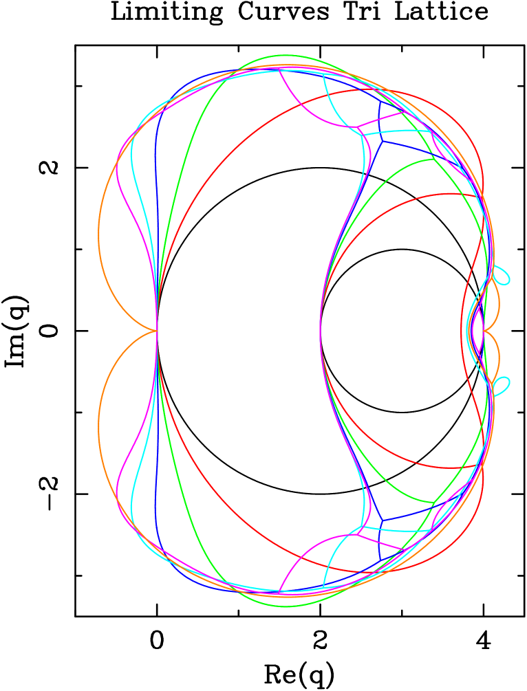
Figure 10: Limiting curves for triangular-lattice strips of width $L$ and toroidal boundary conditions. We show the results for $L=2$ (black), $L=3$ (red), $L=4$ (green), $L=5$ (blue), $L=6$ (light blue), and $L=7$ (pink). We also show the infinite-width limiting curve $\mathcal{B}_{\infty}$ obtained by Baxter [14] (orange).

A summary of qualitative results for the limiting curves $\mathcal{B}$ is shown in Table 7. In Figure 10, we display together all the computed limiting curves $\mathcal{B}_{L}$ with $2\leq L\leq 7$. For comparison, we also include the infinite-volume limiting curve obtained by Baxter [14]. The results in Table 7 with $L\leq 7$ were obtained from the symbolic transfer matrices in Section 4, and those with $L\leq 12$ were found by the numerical procedure outlined in Section 5.1. In all cases $q_{0}(L)$ is given by the crossing between the dominant eigenvalues in the $\ell=0$ and $\ell=2$ sectors.

From the curious fact that $q_{0}(L)=4$ exactly for $L=2,4,5,7,8,10,11$ we conjecture that:

Conjecture 5.5

For triangular-lattice strips with fully periodic boundary conditions, and for all widths $L=3p\pm 1$ with $p\geq 1$, we have $q_{0}(L)=4$.

A quick glance at Table 7 however reveals that the values of $q_{0}(L=3p)$ are definitely not converging to $4$. We therefore examine the data with $L=3p$ more closely. A first fit with $q_{0}(L)=q_{0}(\text{tri})+AL^{-1/\nu}$ yields $q_{0}(\text{tri})\simeq 3.820$ and $\nu\simeq 0.52$ (See Table 8). This is consistent with the expected value $\nu=1/2$ corresponding to a first-order phase transition (in the variable $q$), as we have already found for the square lattice. Fixing $\nu=1/2$ we then arrive at the final estimate $q_{0}(\text{tri})=3.8196\pm 0.0005$.

Remark. We have performed all the fits reported in this paper using the following method: as the data is essentially exact, we have done a standard least-squares fit with as many data points as the number of unknown parameters $N_{A}$ in the Ansatz, so that in each fit there are no effective degrees of freedom. To estimate the error bars (due to the existence of correction-to-scaling terms not included in the Ansatz), we introduce the parameter $L_{\text{min}}$ such that each fit is performed with $N_{A}$ consecutive data points with $L\geq L_{\text{min}}$. From the variation of the estimates as a function of $L_{\text{min}}$, we deduce the corresponding error bars.

Finally, from the FSS theory of first-order phase transitions [24], we expect that higher corrections-to-scaling terms should be integer powers of $L^{-1/\nu}=L^{-2}$. Thus, we have fitted our data to the improved Ansatz

$$q_{0}(L)\;=\;q_{0}(\text{tri})+AL^{-2}+BL^{-4}$$ (5.1)

The results are displayed in Table 8, and from these we conclude that $q_{0}(\text{tri})=3.8198\pm 0.0006$.

We now recall that the triangular-lattice chromatic polynomial was actually shown by Baxter [14] to be an integrable model. In particular, using coordinate Bethe Ansatz, this author identified three different analytic expressions for the free energy in the thermodynamic limit.

To be precise, Baxter used first the Nienhuis mapping [41] between the zero-temperature $q$-state Potts antiferromagnet on the triangular lattice and the critical O($n$) loop model on the hexagonal lattice. That mapping includes an exact relation between $q$ and the weight $n$ of a (bulk) loop. Baxter then transformed the loop model into a vertex model, by the usual trick of redistributing the loop weight $n$ as local complex vertex weights. Unfortunately, when imposing periodic transverse boundary conditions on the vertex model, the loops of non-trivial homotopy (i.e., that wrap around the periodic direction) get the incorrect weight of $2$, a fact not mentioned in Baxter’s paper. Actually, while giving a (boundary) weight of $n^{\prime}=n$ to those loops (by twisting the vertex model) would have been a nicer way to perform the analysis of the O($n$) model, the subtleties of the Nienhuis mapping [41] are such that yet a different weight $n^{\prime}(q)\neq n$ would have been needed to ensure that clusters of non-trivial homotopy in the Potts antiferromagnet carry their correct weight of $q$.

One might think that these subtleties have no implications on the behavior in the thermodynamic limit, but the reader is reminded that we are here dealing with the antiferromagnetic regime in which boundary conditions can (and sometimes do) matter. Nevertheless, it seems reasonable to expect that this should have no consequence for the bulk free energies. Numerical analysis [14, 13] of Baxter’s analytically determined free energies shows that the corresponding eigenvalues become equimodular at

$$q_{\text{B}}\simeq 3.8196717312\,.$$ (5.2)

The value (5.2) is determined implicitly by equating two analytical expressions given in Ref. [14]. Given the excellent agreement with our above numerical determination of $q_{0}(\text{tri})$ we can therefore conjecture that:

Conjecture 5.6

For triangular-lattice strips with fully periodic boundary conditions of widths $L=3p$, the limit $q_{0}({\rm tri})=\displaystyle\lim_{p\to\infty}q_{0}(L)$ exists and is equal to $q_{\text{B}}$ of Eq. (5.2). Furthermore, the sequence $q_{0}(3p)$ is monotonically increasing in $p$.

The number of regions enclosed by $\mathcal{B}$ having a non-zero intersection with the real $q$-axis is $2$ for $L=2,3,4$ [cf. Figure 7 and Table 7]. However, for $L=5$ a further such region appears, whose intersecting with the real $q$-axis is the interval $(q_{2}(L),q_{0}(L))$, where $q_{2}(L)\simeq 3.84826329$. The value $q_{2}(L)$ corresponds to the crossing of the two largest eigenvalues in the $\ell=2$ sector and is tabulated for strip widths $L\leq 12$ in Table 7. This table gives compelling evidence that $q_{2}(L)$ tends to a limit, $q_{2}({\rm tri})<4$, independently of the parity of $L\mathop{\rm mod}\nolimits 3$.

As above, we first fit the data for $q_{2}(L)$ with a fixed parity, $L\mathop{\rm mod}\nolimits 3=0$, to the form $q_{2}(L)=q_{2}(\text{tri})+AL^{-1/\nu}$ (See Table 8). This is again favourable of $\nu\approx 1/2$. Repeating the fit with a fixed $\nu=1/2$ we arrive at the final estimate $q_{2}(\text{tri})=3.8194\pm 0.0016$. Using the improved Ansatz (5.1), we get the value $q_{2}(\text{tri})=3.8199\pm 0.0017$. We can therefore conjecture that:

Conjecture 5.7

For triangular-lattice strips with fully periodic boundary conditions the limit $q_{2}({\rm tri})=\displaystyle\lim_{L\to\infty}q_{2}(L)$ exists and is equal to $q_{\text{B}}$ of Eq. (5.2). Furthermore, the sequence $q_{2}(3p)$ is monotonically decreasing in $p$.

The monotonic nature of the sequences $q_{0}(\text{tri})$ and $q_{2}(\text{tri})$, and the existence of a common limit (as stated in Conjectures 5.6–5.7), means that this common limit is bounded by the finite-widths values: i.e., $q_{0}(3p)\leq q_{\text{B}}\leq q_{2}(3p)$ for all $p\geq 2$. The data for $L=12$ displayed in Table 7 implies that

$$3.81314\;\mathrel{\hbox to0.0pt{\lower 3.0pt\hbox{$\mathchar 536\relax$}\hss}\raise 2.0pt\hbox{$\mathchar 316\relax$}}\;q_{\text{B}}\;\mathrel{\hbox to0.0pt{\lower 3.0pt\hbox{$\mathchar 536\relax$}\hss}\raise 2.0pt\hbox{$\mathchar 316\relax$}}\;3.82428$$ (5.3)

In particular, this narrow interval excludes that this common limit would be equal to the value $q_{\text{G}}=B_{12}$ (1.12) proposed in Ref. [9].

As for the square-lattice case, the limiting curves $\mathcal{B}_{L}$ for $2\leq L\leq 7$ show some regularities (see Figure 10): for real $q$, we have up to four different phases belonging to only three different $\ell$ sectors ($\ell=0,1,2$). Again, within each phase, the leading amplitude does not depend on $L$. All our empirical findings can be summarized in the following conjecture:

Conjecture 5.8

The phase diagram of the zero-temperature triangular-lattice Potts antiferromagnet with toroidal boundary conditions at real $q$ has four different phases characterized by the number of bridges $\ell$ as follows:

• $q\in(-\infty,0)\cup(q_{0}(L),\infty)$ characterized by $\ell=0$ with amplitude $b^{(0)}=1$

• $q\in(0,2)$ characterized by $\ell=1$ with amplitude $b^{(1)}=q-1$

• $q\in(2,q_{2}(L))$ characterized by $\ell=2$ with amplitude $b^{(2)}_{1}=q(q-3)/2$

• $q\in(q_{2}(L),q_{0}(L))$ characterized by $\ell=2$ with amplitude $b^{(2)}_{1}=q(q-3)/2$

Note that the phase (d) only appears for finite width $L$ whenever $q_{0}(L)>q_{2}(L)$ (e.g. $L=5,7$). But, according to Conjectures 5.5–5.7, this phase does survive in the thermodynamic limit $L\to\infty$. We believe that this phase will appear for all $L\geq 5$ such that $L\mathop{\rm mod}\nolimits 3\neq 0$.

For $5\leq L\leq 7$ we further note the appearance of two disjoint triangular-shaped complex-conjugate enclosed regions, whose boundary contains three T points, one of which belongs to the branch of $\mathcal{B}$ that contains the point $q=2$. The dominant eigenvalue inside these enclosed regions comes from the $\ell=0$ sector. Figures 7–8 provide some evidence that these regions may subsist in the thermodynamic limit.

Finally, for $L=6$ we note the emergence of a pair of complex-conjugate enclosed regions analogous to those found for the square lattice. More precisely, these enclosed regions contain points for which $\mathop{\rm Re}\nolimits q>4$, and the corresponding dominant eigenvalue comes from the $\ell=1$ sector. We find it likely that such regions will appear for all $L=3p$ with $p\geq 2$, and will merge in the $L\to\infty$ limit so as to form a branch that intersects the real $q$-axis in $q=q_{0}(\text{tri})=4$.

There is a analogous conjecture for the triangular lattice to Conjecture 5.4 about one of the eigenvalues of the highest sector:

Conjecture 5.9

The diagonal sub-block $T_{L,L}$ for a triangular-lattice strip with fully toroidal boundary conditions and width $L$ contains the eigenvalue $\lambda=(-1)^{L}\,2$ with amplitude $b_{1}^{(L)}$.

5.3 Triangular-lattice free energy

In this section we will discuss the free energy for the triangular-lattice strips we have considered and its relation to the analytic eigenvalues found by Baxter [14].

The (real part of the) free energy per unit area $f_{L}(q)$ for a triangular-lattice strip of width $L$ is given by

$$f_{L}(q)\;=\;\frac{1}{L\,G}\,\log\left|\lambda_{\star}(L;q)\right|$$ (5.4)

where $\lambda_{\star}(L;q)$ is the dominant eigenvalue of the transfer matrix ${\mathsf{T}}(L)$, and $G$ is the geometric factor [c.f., [9, 10]]

$$G(\text{tri})\;=\;\frac{\sqrt{3}}{2}$$ (5.5)

relating the free energy per unit area and per spin. With this normalization the FSS of the free energy is given by

$$f_{L}(q)\;=\;f_{\text{bulk}}(q)+\frac{c(q)\pi}{6\,L^{2}}+\cdots$$ (5.6)

where $f_{\text{bulk}}$ is the bulk free energy per unit area (which is expected to be independent of boundary conditions), $c(q)$ is the (effective) central charge, and the dots stand for higher-order corrections depending on the value of $q$ (in particular, CFT predicts a non-universal $L^{-4}$ correction term).

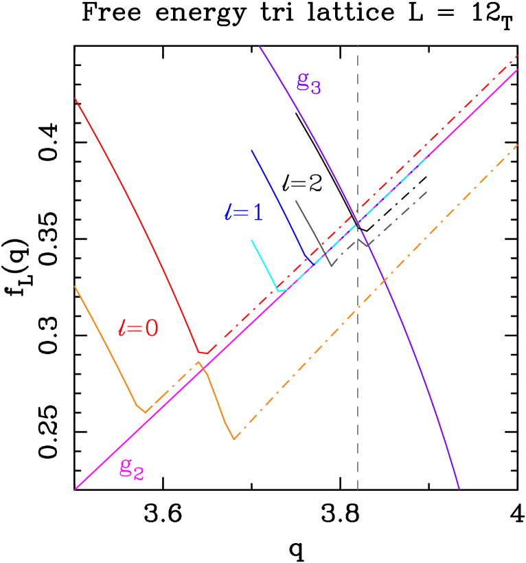
Figure 11: Free energy per unit area $f_{L}(q)$ for the triangular-lattice chromatic polynomial on an infinitely long strip of width $L=12$ and toroidal boundary conditions. We show the free energy $f_{L}(q)$ associated to a selected set of eigenvalues of the transfer matrix ${\mathsf{T}}(12_{\text{T}})$ as a function of $q\in(3.5,4)$. For each sector $\ell=0,1,2$, we show the dominant and the first sub-dominant eigenvalues respectively with colors red/orange for $\ell=0$, blue/cyan for $\ell=1$, and black/dark gray for $\ell=3$. Those eigenvalues that are decreasing (resp.  increasing) in $q$ are depicted with a solid (resp. dot-dashed) curve. For comparison, we also show Baxter’s free energies $(1/G)\log g_{2}$ and $(1/G)\log g_{3}$ [14] normalized per unit area and depicted as solid pink and violet, respectively. The vertical dashed dark gray line shows Baxter’s value $q_{\text{B}}$ (1.11).

In Figure 11, we have plotted the two most dominant free energies for each of the three first sectors $\ell=0,1,2$ for a triangular-lattice strip of width $L=12$ around $q=q_{\text{B}}$ (1.11). The other sectors $\ell\geq 3$ are always sub-dominant and play no role in this discussion. The relevant eigenvalue crossing occurs at $q=q_{0}(L=12)\approx 3.8131463701<q_{\text{B}}$ where the dominant eigenvalue changes from the $\ell=2$ sector (solid black line) to the $\ell=0$ sector (dot-dashed red line). There is also a crossing between the two most dominant $\ell=2$ eigenvalues at $q=q_{2}(L=12)\approx 3.82428323>q_{\text{B}}$. This crossing gives rise to a new $\ell=2$ phase (between $q_{0}$ and $q_{2}$) for all strips of width not a multiple of three. In both cases, the $\ell=1$ sector plays no role in the phase structure around $q=q_{\text{B}}$. This computation gives numerical evidence that our scenario is correct and no new elements are at play.

Another interesting question is whether the bulk free energy $f_{\text{bulk}}(q)$ agrees or not with Baxter’s free energies per unit area $(1/G)\log|g_{i}|$ ($i=1,2,3$) [14]. (See Ref. [13, Section 6.1] for a detailed description of Baxter’s solution). In particular, Baxter found that the free energy is given by $g_{3}$ in the region containing the interval $q\in(0,q_{\text{B}})$, by $g_{2}$ in the region containing the interval $q\in(q_{\text{B}},4)$, and by $g_{1}$ in the rest of the complex $q$-plane.

In Figure 11 we observe that the agreement with Baxter’s solution is very good: for $q\mathrel{\hbox to0.0pt{\lower 3.0pt\hbox{$\mathchar 536\relax$}\hss}\raise 2.0pt\hbox{$\mathchar 318\relax$}}q_{\text{B}}$ the free energy is very similar to the $g_{2}$ contribution (actually it seems to be almost equal to the contribution of the $\ell=1$ sector), while for $q\mathrel{\hbox to0.0pt{\lower 3.0pt\hbox{$\mathchar 536\relax$}\hss}\raise 2.0pt\hbox{$\mathchar 316\relax$}}q_{\text{B}}$, it is similar to the contribution of $g_{3}$.

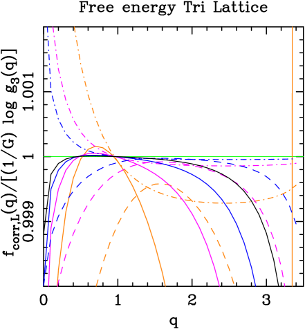
(((a)(a)	(((a)(b)

Figure 12: Ratios of the free energy per unit area for an infinitely long triangular-lattice strip of width $L$ and toroidal boundary conditions and Baxter’s free energy per unit area $(1/G)\log g_{3}(q)$ [14]. (a) Ratio of the free energy per unit area $f_{L}(q)$ (5.4). (b) Ratio of the corrected free energy per unit area $f_{\text{corr},L}(q)$ (5.7). For each strip width $L=6$ (orange), $L=9$ (pink), $L=12$ (blue), and $L=15$ (black), we show the ratio of the free energies associated to the first three levels $\ell=0$ (solid line), $\ell=1$ (dashed line), and $\ell=2$ (dot-dashed lines).

A striking difference between our phase-transition diagrams and Baxter’s solution is the transition line going through $q=2$, which is absent in the latter. This line separates the phase characterized by $\ell=1$ from the one characterized by $\ell=2$ (which agrees with Baxter’s solution close to $q=q_{\text{B}}$). Therefore a natural question is whether there is one eigenvalue missing in Baxter’s solution and corresponding to the $\ell=1$ sector. To answer this question we have plotted in Figure 12(a) the ratio of the free energy per unit area $f_{L}(q)$ and Baxter’s free energy $(1/G)\log g_{3}(q)$ in the interval $q\in(0,3.5)$. To avoid parity effects, we have considered only lattices of widths $L=3p$ with $p=2,3,4,5$, and for each width we have considered the free-energy contribution from the three lowest sectors $\ell=0,1,2$ (represented by solid, dashed, and dot-dashed curves, respectively).

Note that the eigenvalue crossings occur at the points $q=0,2$. Another exact crossing, involving the second and third most dominant eigenvalues, takes place at $q=1$. The fact that the loci of these crossings are subject to no finite-size corrections can presumably be explained using quantum group arguments.

The numerical agreement with $g_{3}$ is not very good as the ratio is consistently below the expected result (i.e., $1$). The reason is that the FSS corrections (5.6) have not been taken into account. A better agreement can be obtained if we take into account the first correction term in (5.6). We then define the corrected free energy per unit area

$$f_{\text{corr},L}(q)\;=\;f_{L}(q)-\frac{\pi c_{\rm eff}(q)}{6\,L^{2}}\;=\;f_{\text{bulk}}(q)+o\left(L^{-2}\right)$$ (5.7)

where $c_{\rm eff}(q)$ is the effective central charge for the BK phase discussed in the next section; see (5.14). We expect that this value will be closer to the thermodynamic limit $f_{\text{bulk}}(q)$, as the correction terms are $o(L^{-2})$. This plot is shown in Figure 12(b). Our first observation is that the values of the ratio are much closer to the expected value of $1$ than in Figure 12(a). This shows that our assumption that CFT holds for this model is valid. Note that the eigenvalue crossings do not need to be at the expected points $q=0,2$, as the correction in (5.7) depends on both $q$ and $L$. The second observation is that the agreement of the $\ell=2$ free energy with the contribution of $g_{3}$ is very good for $q\mathrel{\hbox to0.0pt{\lower 3.0pt\hbox{$\mathchar 536\relax$}\hss}\raise 2.0pt\hbox{$\mathchar 318\relax$}}1$ (less than $0.02\%$ for $L=9,12$). For $q\mathrel{\hbox to0.0pt{\lower 3.0pt\hbox{$\mathchar 536\relax$}\hss}\raise 2.0pt\hbox{$\mathchar 316\relax$}}1$, the best agreement corresponds to the $\ell=0$ sector. However, it is difficult from this data alone to draw any definitive conclusion about the necessity of including an extra eigenvalue to the set introduced by Baxter.

5.4 Conformal properties

Following Refs. [29, 30] we expect a number of the conformal properties of the chromatic polynomial to be given by the BK antiferromagnetic phase. In brief, the situation is the following. The two-dimensional Potts model is exactly solvable (i.e., integrable) on the curves

$$\begin{array}[]{ll}v=\pm\sqrt{q}&\mbox{(square lattice)}\\[5.69054pt] v^{3}+3v^{2}=q&\mbox{(triangular lattice)}\end{array}$$ (5.8)

The part of the curves with $0\leq q\leq 4$ and $v\geq 0$ corresponds to the usual second-order transition between a ferromagnetic and a paramagnetic phase. Its critical properties are given by the Coulomb gas (free field) construction with coupling constant $g\in[0,1/2]$; in particular the thermal operator (corresponding to a perturbation of the critical point in the $v$ variable) is relevant in the RG sense. Now, the analytic continuation to the region with $g\in(1/2,1)$ describes the lower (resp. middle) branch of the curves (5.8) for the square (resp. triangular) lattice. Crucially, at these critical points the thermal operator is irrelevant. Therefore, for each value of $q\in(0,4)$, these critical points will act as an RG attractor for a finite interval $(v_{-}(q),v_{+}(q))$: this is the BK phase. For the square lattice, the end-points of these intervals are given by the two mutually dual antiferromagnetic phase transition points [31]

$$v_{\pm}(q)=-2\pm\sqrt{4-q}$$ (5.9)

whereas for the triangular lattice $v_{\pm}(q)$ are presently unknown.

The upshot is that the part of the chromatic line $v=-1$ that intersects the BK phase will have its critical properties determined by the latter. For the square lattice this happens for $\mathop{\rm Re}\nolimits q\in(0,3)$, according to Eq. (5.9), in perfect agreement with Conjecture 5.2. For the triangular lattice, we obtain a consistent scenario if we suppose that the intersection with the BK phase is for $\mathop{\rm Re}\nolimits q\in(0,q_{2})$, with $q_{2}$ given by Conjecture 5.7.

Within the BK phase, we can parametrize $q$ by

$$q\;=\;4\cos^{2}\left(\frac{\pi}{p}\right)$$ (5.10)

where $p\in(2,\infty)$. The central charge is then

$$c(p)=1-\frac{6(p-1)^{2}}{p}.$$ (5.11)

Furthermore, the theory possesses an infinite set of bulk operators $\mathcal{O}_{k}$, with $k=1,2,\ldots$, of conformal weight [42]

$$h_{k}(p)=\frac{k^{2}-(p-1)^{2}}{4p}.$$ (5.12)

Geometrically, the insertion of an $\mathcal{O}_{k}$ operator at either end of the strip corresponds to a situation in which $2k$ cluster boundaries propagate along the length direction of the strip. (The boundaries may of course also wind around the periodic transverse direction.) For $k\geq 2$ we may equivalently think of $k$ propagating clusters. It should be carefully noted that the case $k=1$ is special: a single propagating cluster may either correspond to two or zero propagating cluster boundaries. The latter case will occur when the cluster is allowed to have cross-topology [43], i.e., to percolate across both periodic lattice directions. The corresponding bulk operator is denoted $\tilde{\mathcal{O}}_{1}$ and has conformal weight

$$\tilde{h}_{1}(p)=\frac{-3p^{2}+8p-4}{16p}.$$ (5.13)

Indeed, by duality this is nothing else than the order parameter (magnetization) operator.

In the probabilistic regime (i.e., $v>0$) the identity operator $\mathcal{I}$ is the most relevant (all other conformal weights are strictly positive). Similarly, one has $\tilde{h}_{1}<h_{1}$, translating the fact that a single cluster is indeed most likely to have cross-topology. In the BK phase, $v<0$ and some of these statements need no longer be true, due to the presence of negative conformal weights. In fact, for any $p>2$ the weight $h_{1}$ is the most negative, and so one would naively expect that the most “likely” configurations are those with two propagating cluster boundaries. This is however not true, due to a subtle effect: the amplitudes of the corresponding transfer matrix eigenvalues vanish identically on the torus [30]!

So the remaining candidates for the most relevant operators are $\tilde{\mathcal{O}}_{1}$ and $\mathcal{O}_{2}$. From Eqs. (5.12)–(5.13) it is easy to see that the former (resp. the latter) will dominate for $2<p<4$ (resp. for $4<p<\infty$). This argument is of course valid in the thermodynamic limit only, but the conclusion will in fact hold true in finite size due to the underlying quantum group symmetry of the model. Accordingly we indeed observe numerically, for any width $L$ and for both lattices, that branches of the limiting curves $\mathcal{B}$ cross the real $q$-axis at $q=0$ ($p=2$) and $q=2$ ($p=4$); the former (resp. the latter) crossing corresponds to the equimodularity of the dominant eigenvalues of the $\ell=0$ and $\ell=1$ (resp. the $\ell=1$ and $\ell=2$) sectors. However, the phase containing $q=2^{+}$ does not extend to $q=4$ ($p=\infty$) for either lattice, since the chromatic line leaves the BK phase at $q_{0}=3$ (square lattice), respectively $q_{2}\simeq 3.8196717312$ (triangular lattice).

We can further check the validity of this scenario by turning to the amplitudes of the dominant eigenvalues. For the order parameter operator $\tilde{\mathcal{O}}_{1}$ the amplitude is $q-1$ (by a simple counting argument), and this is indeed the amplitude of the dominant eigenvalue observed numerically for $p\in(2,4)$ for both lattices. (See Conjectures 5.3(b) and 5.8(b).) For the two-cluster operator $\mathcal{O}_{2}$ the amplitude should be either $b^{(2)}_{1}$ or $b^{(2)}_{2}$ [cf. Eqs. (LABEL:def_b21)–(LABEL:def_b22)]. And indeed the amplitude of the eigenvalues which is dominant in the phase containing $q=2^{+}$ is observed numerically to be $b^{(2)}_{1}$. (See Conjectures 5.3(c) and 5.8(c).) As a last check, note that from Eqs. (5.12)–(5.13) the effective central charge should read

$$c_{\text{eff}}(q)\;=\;\begin{cases}\displaystyle\;1-\frac{3p}{2}&\qquad\text{for $2<p<4$}\\[11.38109pt] \displaystyle\;1-\frac{24}{p}&\qquad\text{for $4<p<p_{0}$}\end{cases}$$ (5.14)

We have checked numerically that this is true on both lattices (using strips of width $L\leq 12$) to a very good precision; this check is essentially the contents of Figure 12(b).

A final elusive point is the value of $c$ in the interval $q\in(q_{2},q_{0})$ on the triangular lattice. The $q_{0}(\text{tri})=4$ case is known to be equivalent to Baxter’s three-colouring problem on the hexagonal lattice and hence have $c=2$. Our numerical data seem to indicate that the rest of the interval $(q_{2},q_{0})$ may also correspond to a critical theory, the properties of which are unrelated to those of the BK phase.

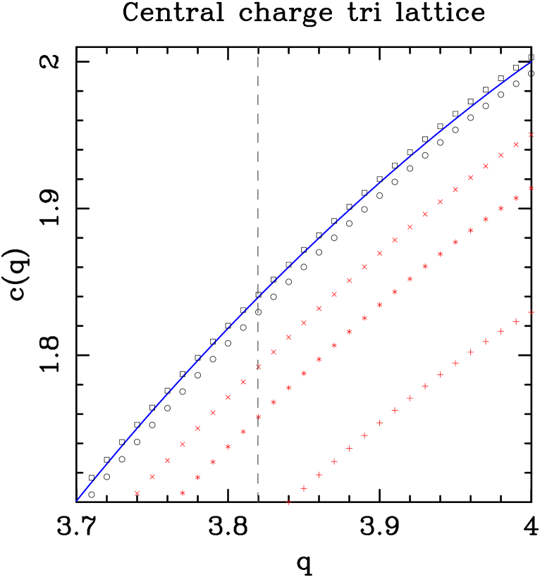
Figure 13: Central charge for the triangular-lattice chromatic polynomial on infinitely long strips with toroidal boundary conditions. We show several two-parameter fits (depicted in red): $L=6,9$ ($+$), $L=9,12$ ($\star$), and $L=12,15$ ($\times$). We also show three-parameter fits using the Ansatz (5.15) (depicted in black): $L=6,9,12$ ($\circ$), and $L=9,12,15$ ($\square$). The solid blue line represents our guess for the central charge (5.16). The vertical dashed dark gray line shows Baxter’s value $q_{\text{B}}$ (1.11).

We have made an attempt to obtain an expression for the central charge in the interval $q\in(q_{2},q_{0})$ by performing some fits to our free-energy data. Our first two-parameter Ansatz was given by Eq. (5.6) without any correction-to-scaling term. In Figure 13 we show our estimates as a function of $q$ for different values of $L_{\text{min}}=6,9,12$. Much better estimates can be obtained by including higher-order corrections to the above Ansatz. In previous work [13, 9, 10], we have found that including a correction term $\sim L^{-4}$ greatly improves the estimates for the central charge. Thus, we have used the improved three-parameter Ansatz

$$f_{L}(q)\;=\;f_{\text{bulk}}(q)+\frac{\pi c(q)}{6\,L^{2}}+A\,L^{-4}$$ (5.15)

In Figure 13 we have also displayed the estimates for $c(q)$ obtained with this Ansatz and $L_{\text{min}}=6,9$. Their stability is superior to that of the two-parameter estimates. The solid line represents a guess for the exact value of the (effective) central charge in this regime (see (5.19) below)

$$c(q)\;=\;2-\frac{28}{p^{2}-2p-12}$$ (5.16)

where $p\in(2,\infty)$ is related to $q$ by (5.10).

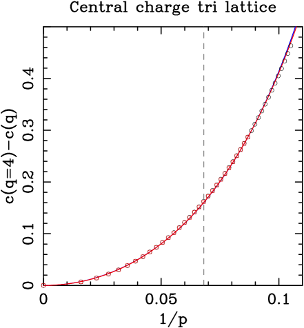
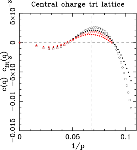
(((a)(a)	(((a)(b)

Figure 14: Central charge for the triangular-lattice chromatic polynomial on infinitely long strips with toroidal boundary conditions. (a) Difference $c(q=4)-c(q)$ as a function of $1/p$ [c.f., (5.10)]. We show two estimates coming from the three-parameter fits (5.15) with $L=6,9,12$ (black $\circ$) and $L=9,12,15$ (red $\square$). The (almost coincident) solid lines represent our two best candidates for the central charge (LABEL:def_c_diff_conjectured1) (blue), and (LABEL:def_c_diff_conjectured2) (red). (b) Error between our numerical estimates for the conformal charge and our conjectured expressions (5.16). We show the difference $c(q)-c_{\text{fit}}(q)$ between our three-parameter fits and our conjectured expressions $c_{\text{fit}}(q)$. Points in black (resp. red) are obtained from the fits with $L=6,9,12$ (resp. $L=9,12,15$). Solid [resp.  empty] symbols are obtained with $c_{\text{fit}}$ given by (LABEL:def_c_diff_conjectured1) [resp.  (LABEL:def_c_diff_conjectured2)]. In both plots, the vertical dashed dark gray line shows Baxter’s value $1/p_{\text{B}}\approx 0.0681036688$ obtained from (1.11)/(5.10).

Let us now explain in detail how we have obtained the expression (5.16). The functional form of the Ansatz (5.16) is motivated by already known results of the central charge in other regimes [c.f., (5.11)]. Thus, our goal is to obtain the central charge $c(q)$ as a rational function of $p$ with integer coefficients. We started with the estimates coming from the three-parameter Ansatz (5.15). It is more useful to plot the results as a function of $1/p$, so that $q=4$ ($p=\infty$) corresponds to the origin. In Figure 14(a) we display the difference $c(q=4)-c(q)$ versus $1/p$ for the two available data sets $L_{\text{min}}=6,9$. Both data sets fall approximately on a single curve, especially on the interval corresponding to $q\in(q_{2},q_{0})$. This empirical result implies that the largest FSS correction to our estimates for $c(q)$ corresponds to a global shift. We then fit the data for $c(q=4)-c(q)$ to a polynomial Ansatz. Our best result is given by

$$c(q=4)-c(q)\;=\;28.60506\frac{1}{p^{2}}+32.11981\frac{1}{p^{3}}+897.88358\frac{1}{p^{4}}$$ (5.17)

This Ansatz is motivated by several facts: by definition, the curve should go through the origin, and it is clear in Figure 14(a) that its slope at $1/p=0$ is zero. Furthermore, the addition of more terms to (5.17) only leads to less stable estimates. As our goal is to obtain a rational function of $p$, we computed the Padé approximant $[2,2]$ of the above polynomial (5.17). The result is given by

$$c(q=4)-c(q)\;=\;\frac{28.60506}{p^{2}-1.12287p-30.12813}$$ (5.18)

Finally, as we expect that the coefficients of the above rational function are integers, we systematically searched the set of closest integers which best approximates the data of Figure 14(a). Our best candidates were

$$c(q=4)-c(q)&=\frac{28}{p^{2}-2p-12}{}\\ c(q=4)-c(q)=\frac{29}{p^{2}-p-20}{}$$ (5.19)

In Figure 14(a) it is clear that both expressions give an excellent fit to the whole set of data points. In order to tell which integer-coefficient rational approximant was best, we plotted the difference between our estimates and the fits. In Figure 14(b) we show this difference for the above approximants (5.19). We observe that the approximant (LABEL:def_c_diff_conjectured1) is slightly superior to the other one (LABEL:def_c_diff_conjectured2).

The final step is to fix the overall shift, i.e., the value of $c(q=4)$. As the triangular-lattice Potts antiferromagnet at zero temperature is critical and can be mapped onto a Gaussian model with two bosons [44, 45], we expect that

$$c(q=4)\;=\;2$$ (5.20)

Thus, we arrive at the final expression (5.16). Indeed, this computation should be taken with a grain of salt: we have found a function with the expected properties (rational function of $p$ with integer coefficients) that describes rather accurately our estimates for the central charge of our model on the interval $q\in(q_{2},q_{0})$. This does not mean that this is unique possible solution with those properties nor that the right expression for $c(q)$ should satisfy those properties. Another important point is that our conjectured expression for the central charge, although it was first devised to deal with the interval $q\in(q_{2},q_{0})$, is able to reproduce rather accurately the data outside the latter interval.

5.5 The “$\bm{q=2}$ branch”

At the end of Section 5.3, we have already discussed the branch of the triangular-lattice limiting curve $\mathcal{B}_{L}$ going through the point $q=2$, and separating the $\ell=1$ and $\ell=2$ phases. In this subsection we will study further properties of this branch in both the square and triangular limiting curves.

The first question we want to address is that of the density of chromatic zeros along this branch for finite strips of size $L\times N$. In order to estimate this density, we first fixed a region in the complex $q$-plane containing the $q=2$ branch. This region is

$$\text{Sq}&\Rightarrow 1.8\;\leq\;\mathop{\rm Re}\nolimits q\;\leq\;2.2\,,\qquad|\mathop{\rm Im}\nolimits q|\;\leq\;1.2\\ \text{Tri}\Rightarrow 1.8\;\leq\;\mathop{\rm Re}\nolimits q\;\leq\;2.6\,,\qquad|\mathop{\rm Im}\nolimits q|\;\leq\;1.4$$ (5.21)

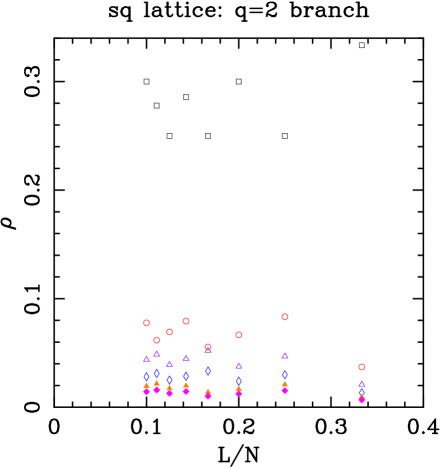
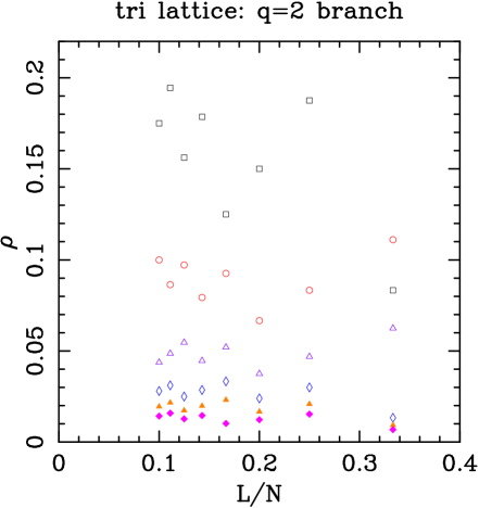
(((a)(a)	(((a)(b)

Figure 15: Density of chromatic zeros for (a) square- and (b) triangular-lattice strips with toroidal boundary conditions along the $q=2$ branch of the limiting curve $\mathcal{B}_{L}$. In order to compute the density of zeros, We have considered the regions given by (5.21). For a given lattice strip of width $L$ and length $N$, we plot the ratio of zeros falling in the respective region as a function of the inverse aspect ratio (i.e., $L/N$). The widths are $L=2$ (black $\square$), $L=3$ (red $\circ$), $L=4$ (violet $\triangle$), $L=5$ (blue $\diamond$), $L=6$ (orange $\blacktriangle$), and $L=7$ (pink $\blacklozenge$).

In Figure 15, we show the density of the chromatic zeros $\rho$ in the regions (5.21) for some finite strips of size $L\times N$ as a function of the aspect ratio $L/N$. At fixed aspect ratio, we expect the density $\rho$ to converge to some (small) positive constant. In Figure 15, we observe that for fixed $L/N$, the density is decreasing in $L$, and it attains at $L=7$ very small values $\mathrel{\hbox to0.0pt{\lower 3.0pt\hbox{$\mathchar 536\relax$}\hss}\raise 2.0pt\hbox{$\mathchar 316\relax$}}0.02$. If this monotonicity holds for larger values of $L$, we expect that the density of zeros along the $q=2$ branch will converge to zero in the thermodynamic limit (in contrast with the behavior of the density of zeros in other parts of the limiting curve).

Another way to tackle this problem is consider the parameter $t$ introduced in Ref. [11, Section 4.1.1]. On the limiting curve $\mathcal{B}_{L}$, there are generically two equimodular leading eigenvalues $\lambda_{1}$ and $\lambda_{2}$. Indeed, their ratio is just a phase

$$\frac{\lambda_{1}}{\lambda_{2}}\;=\;e^{i\,\theta}\,,\qquad\theta\in{\mathbb{R}}$$ (5.22)

In Ref. [11], instead of $\theta$, we found it more convenient to work with the real parameter $t$, defined as

$$t\;=\;\tan\left(\frac{\theta}{2}\right)\,,\qquad t\in[0,\infty)$$ (5.23)

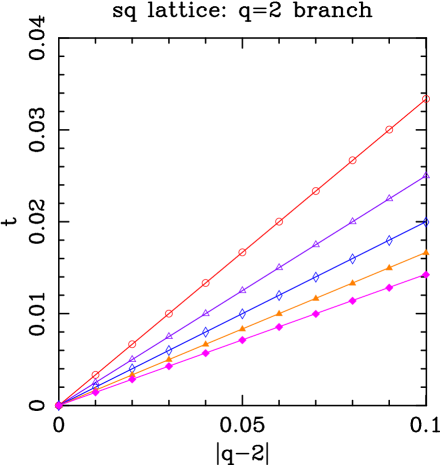
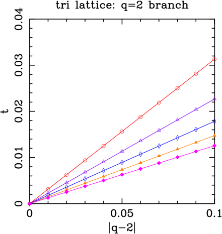
(((a)(a)	(((a)(b)

Figure 16: Values of the parameter $t$ (5.23) along the $q=2$ branch of the limiting curve $\mathcal{B}_{L}$ for the (a) square- and (b) triangular-lattice strip. For a lattice strip of width $L$, we show the value of $t$ as a function of $|q-2|$. The widths are $L=3$ (red $\circ$), $L=4$ (violet $\triangle$), $L=5$ (blue $\diamond$), $L=6$ (orange $\blacktriangle$), and $L=7$ (pink $\blacklozenge$). The slopes of the depicted lines are given approximately by $1/L$ (square) and $\sqrt{3}/(2L)+0.653/L^{3}$ (triangular).

In practice, we use this parameter to ensure the plots of the limiting curves $\mathcal{B}_{L}$ are correct and we do not miss any small feature. Note that $t=\theta=0$ corresponds to two identical eigenvalues. At $q=2$, we have that $t=0$ for any $L\geq 3$; but as we move along the $q=2$ branch, $t$ increases. Let us now study how the parameter $t$ evolves (along this branch) as a function of $|q-2|$. In Figure 16, we show (for both the square and triangular lattices) the values of $t$ along the $q=2$ branch for points in the complex $q$-plane with $\mathop{\rm Im}\nolimits q=0,0.01,\ldots,0.10$. It is clear that for fixed $L$, the relation is approximately linear. For the square lattice, the slope is given approximately by $1/L$, while for the triangular lattice the slope is given approximately by $\sqrt{3}/(2L)+0.653/L^{3}$. In both cases, the discrepancies between the estimated slopes and the above results are of order $O(10^{-4})$. Thus, we expect that in the thermodynamic limit both leading eigenvalues $\lambda_{1}$ and $\lambda_{2}$ become equal along this branch.

Finally, we can study the behavior at $q=2$ by considering the series expansion of the two equimodular leading eigenvalues $\lambda_{1}$ and $\lambda_{2}$ (corresponding to the $\ell=1$ and $\ell=2$ sectors, respectively). Indeed, such series expansions are expected to exist, as the eigenvalues $\lambda_{i}(q)$ are algebraic functions of $q$. On each phase, we can compute the series expansion of the leading eigenvalue at $q=2+\epsilon$

$$\lambda_{i}(q+\epsilon)\;=\;\sum\limits_{k=0}^{\infty}\lambda_{i,k}\,\epsilon^{k}$$ (5.24)

For $L=2,3$, this can be done symbolically by using mathematica. For $4\leq L\leq 7$, we can only obtain (again with mathematica) the series numerically, as the symbolic expressions for the coefficients are too lengthy. In practice, we are able to obtain the first three coefficients $\lambda_{i,k}$ ($k=0,1,2$) in (5.24). With these coefficients, we can obtain the corresponding series expansion for the free energy:

$$f_{L}(2+\epsilon)\;=\;\begin{cases}\frac{1}{L}\log|\lambda_{1}(2+\epsilon)|\;=\;\sum\limits_{k=0}^{\infty}f_{L,k}^{(1)}\,\epsilon^{k}&\quad\text{if $\epsilon\leq 0$}\\[11.38109pt] \frac{1}{L}\log|\lambda_{2}(2+\epsilon)|\;=\;\sum\limits_{k=0}^{\infty}f_{L,k}^{(2)}\,\epsilon^{k}&\quad\text{if $\epsilon\geq 0$}\end{cases}$$ (5.25)

For $4\leq L\leq 12$, we numerically obtained the contribution to the free energy $f_{L,i}(q)=(1/L)\log|\lambda_{i}(q)|$ of the two leading eigenvalues $\lambda_{i}$ close to $q=2$. In particular, we obtained the values $f_{L,i}(q=2)$ and $f_{L,i}(q=2\pm 10^{-5})$ for $i=1,2$. From these six values, we estimated the first three coefficients $f^{(i)}_{L,k}$ (with $k=0,1,2$) in (5.25). Indeed, we know that the free energy is continuous at $q=2$, thus we expect that $\Delta f_{L}(2)=f_{L,0}^{(2)}-f_{L,0}^{(1)}=0$, as we find in the actual computation. We are interested in computing the increment of the first derivatives of the free energy $f_{L}(q)$ at $q=2$. In practice, we have computed the increments of the first two derivatives:

$$E_{L}&=\Delta\left(\left.\frac{df_{L}}{dq}\right|_{q=2}\right)\;=\;f_{L,1}^{(2)}-f_{L,1}^{(1)}\\ C_{L}=\Delta\left(\left.\frac{d^{2}f_{L}}{dq^{2}}\right|_{q=2}\right)\;=\;2(f_{L,2}^{(2)}-f_{L,2}^{(1)})$$ (5.26)

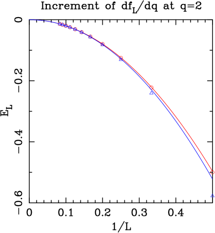
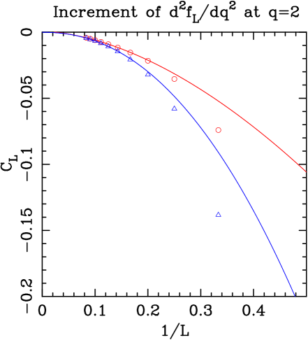
(((a)(a)	(((a)(b)

Figure 17: Coefficients of the series expansions for the increment of the first (a) and second (b) derivatives of the free energy $f_{L}(q)$ with respect to $q$ evaluated at $q=2$. In each plot we show the corresponding coefficient for the square (red $\circ$) and triangular (blue $\triangle$) lattices as a function of $1/L$. The solid lines depict the best power-law fits to the corresponding data set (5.27)/(5.28).

If $E_{L}\neq 0$, then the transition at $q=2$ is of first order. However, if $E_{L}=0$ and $C_{L}\neq 0$, then the transition is of second order (and this argument can be generalized to higher-order phase transitions). In Figure 17 we have plotted the coefficients $E_{L}$ and $C_{L}$ versus $1/L$ for both the square and triangular lattices. The plots suggest that both coefficients for both lattices tend to a limit as $L\to\infty$. If we fit the $E_{L}$–data to a power law $E_{L}=E_{\infty}+A_{E}L^{-\omega_{E}}$, we find that $|E_{\infty}|\mathrel{\hbox to0.0pt{\lower 3.0pt\hbox{$\mathchar 536\relax$}\hss}\raise 2.0pt\hbox{$\mathchar 316\relax$}}10^{-4}$ is indeed very small (in modulus) for $L_{\text{min}}=10$:

$$\text{Sq}&\Rightarrow E_{L}\;\approx\;9.8\times 10^{-7}-1.98329\,L^{-1.99737}\\ \text{Tri}\Rightarrow E_{L}\;\approx\;-0.00010\;-2.12401\,L^{-2.02506}$$ (5.27)

In particular, our square-lattice data can be fitted very well with the simple Ansatz: $E_{L}(\text{sq})=-2L^{-2}$. These fits are depicted in the corresponding plots in Figure 17. We have chosen $L_{\text{min}}$ to be the largest possible value, so that there are no effective degrees of freedom in the fits.

The power-law fits $C_{L}=C_{\infty}+A_{C}L^{-\omega_{C}}$ are not as stable as the preceding ones: we find sizeable parity effects in the estimates, so we have to split the whole data set into two smaller sets with well-defined $L$–parity. Thus, for each value of $L_{\text{min}}$, we have fitted the data with $L=L_{\text{min}},L_{\text{min}}+2,L_{\text{min}}+4$. The estimates for even $L$ are given for $L_{\text{min}}=8$ by:

$$\text{Sq}&\Rightarrow C_{L}\;\approx\;\phantom{-}0.00051-0.35387\,L^{-1.73364}\\ \text{Tri}\Rightarrow C_{L}\;\approx\;-0.00012-0.99690\,L^{-2.18046}$$ (5.28)

For odd $L$ with $L_{\text{min}}=7$, the corresponding estimates are:

$$\text{Sq}&\Rightarrow C_{L}\;\approx\;\phantom{-}0.00116-0.30522\,L^{-1.62941}\\ \text{Tri}\Rightarrow C_{L}\;\approx\;-0.00092-1.42076\,L^{-2.38725}$$ (5.29)

Our preferred fits are those given by (5.28), as $L_{\text{min}}$ is larger; these fits are depicted in the corresponding plots in Figure 17. They also show show that $C_{L}$ tend to some small (in modulus) number in the thermodynamic limit $|C_{\infty}|\mathrel{\hbox to0.0pt{\lower 3.0pt\hbox{$\mathchar 536\relax$}\hss}\raise 2.0pt\hbox{$\mathchar 316\relax$}}5\times 10^{-4}$. We conjecture that for both lattices, $E_{L},C_{L}\to 0$ as $L\to\infty$. Indeed, this does not mean that there is no transition at all at $q=2$ in the thermodynamic limit, but that the transition (if any) is at least of third order.

In this section we have presented three numerical approaches to study the thermodynamic limit along the $q=2$ branch. None of them is conclusive; but taken together they give strong support to the following scenario: even though at finite $L$ there are two different phases coexisting along the $q=2$ branch, in the thermodynamic limit there is a unique phase. This scenario is consistent with the three results discussed above: in the thermodynamic limit $L\to\infty$: 1) The density of chromatic zeros goes to zero along this branch; 2) The ratio of eigenvalues along this branch tend to one $\lambda_{2}/\lambda_{1}\to 1$; and 3) At $q=2$ the increment in the first two derivatives of the free energy $f_{L}(q)$ (with respect to $q$) tends to zero. Thus, this branch seems to be somehow an artifact of the boundary conditions; in particular, of the periodic longitudinal boundary conditions, as this branch also appears in the cyclic case [9], and it is absent for free and cylindrical boundary conditions [11, 12, 13]. This conclusion agrees with Baxter’s solution [14] in the sense that only three phases survive in the phase diagram of the triangular-lattice chromatic polynomial.

6 Conclusions

In this paper we have extended our transfer-matrix studies [11, 12, 13, 9] to toroidal boundary conditions. We have obtained the exact expression of the chromatic polynomial for square- and triangular-lattice strips of fixed width $2\leq L\leq 7$ and arbitrary length $N$. The cases $L=5,6,7$ are new in the literature (note that going to larger widths $L\geq 8$ would require better computer facilities and/or improved symbolic algorithms). We have also obtained the limiting curves $\mathcal{B}_{L}$ and isolated limiting points for these strips in the infinite-length limit $N\to\infty$. The limiting curve $\mathcal{B}_{L}$ for a fixed value of $L$ provides the exact phase diagram for this semi-infinite strip.

By studying the features of these finite-$L$ phase diagrams and using techniques from CFT and FSS, we have been able to determine some properties of the chromatic-polynomial phase diagram in the thermodynamic limit $L\to\infty$. These findings are summarized in the following points:

• Toroidal boundary conditions appear to give results qualitatively and quantitatively closer to those of the thermodynamic limit than the other standard boundary conditions (free, cylindrical, and cyclic) [11, 12, 13, 9]. In particular, the exact value of $q_{c}$ is obtained for all square lattices of (finite) odd widths, and for all triangular lattices of (finite) widths not a multiple of three.

• As for cyclic boundary conditions [9], we find that the limiting curves $\mathcal{B}_{L}$ always enclose regions of the complex $q$-plane, thus determining true phases as in the expected infinite-volume phase diagram. Each phase is also characterized by the number of bridges $\ell$ associated to the leading eigenvalue; but for toroidal boundary conditions only the $\ell=0,1,2$ sectors contribute for both lattices. (For the triangular lattice with cyclic boundary conditions we expect to have contributions up to $\ell=6$ bridges). The other difference with the cyclic triangular strip is that there are now two different phases characterized by $\ell=2$ bridges (For cyclic boundary conditions, there is at most one phase for each value of $\ell$).

• It is rather remarkable that for cyclic boundary conditions [29, 9], all the Beraha numbers $B_{p}$ (1.8) played a special role in the BK phase, either as phase transition points (even $p$) or as isolated limiting points (odd $p$). In contrast, for toroidal boundary conditions only the finite subset of integer $q$ play such special roles: there are phase transitions at $q=0,2,4$ and isolated limiting points at $q=1,3$. This observation alone is a nice illustration of the crucial influence of boundary conditions on antiferromagnetic systems. Note however, that we still expect (and have to some extent numerically observed) that the full set of $B_{p}$ will be the loci of level crossings of sub-dominant eigenvalues.

• Seeing that the maximum chromatic number $H(g)$ of a graph $G$ increases with the genus $g$ of the surface that it is embedded in according to (1.5), one might have expected that the toroidal topology studied here would have revealed further structure of the limiting curves for $q\in(4,7)$. This is not the case. The reason is that it is precisely the interplay between the properties of the BK phase and the representation theory of the quantum group $U_{t}(SU(2))$ for $t$ a root of unity that is responsible for generating the partition-function zeros. This mechanism is confined to the interval $q\in[0,4]$. The graphs having chromatic zeros for $q\in(4,7)$ must therefore be rather exceptional and have little to do with the recursive families of graphs studied here. One might even speculate that the number of such exceptional graphs might be small in some sense, or even finite. These conclusions are expected to carry over to higher genus as well.

• For toroidal triangular strips we have found two phase transitions inside the critical region: $q=2$ and $q=q_{\text{B}}$ (1.11).

  This result is rather puzzling when compared to Baxter’s exact solution [14] and the re-analysis discussed in Ref. [9] of Baxter’s eigenvalues. On one hand, the value of $q_{\text{B}}$ coincides with that predicted by Baxter based on the result that only three eigenvalues are relevant in the complex $q$-plane. This conclusion stems from the Bethe-Ansatz solution of a closely related model [14]. The mapping between these two models is exact, except for the boundary conditions. Usually boundary conditions have no effect in the ferromagnetic regime; but here we are deep in the antiferromagnetic one.

  On the other hand, a careful and high-precision analysis of these three eigenvalues [9] revealed that, although the outer boundary of Baxter’s infinite-volume curve $\mathcal{B}_{\infty}$ was indeed correct, the inner structure was richer: there were infinitely many more branches than those included by Baxter and those indicated by the finite-strip chromatic zeros. In particular, the point $q_{\text{B}}$ (1.11) does not belong to the limiting curve $\mathcal{B}_{\infty}$, and its role is now played by $q_{\text{G}}$ (1.12).

• In Section 5.5 we have found some numerical evidence that the branch of the limiting curves $\mathcal{B}_{L}$ going through $q=2$ might disappear in the true thermodynamic limit $L\to\infty$. This may provide an explanation of why this branch is absent from the triangular-lattice limiting curve $\mathcal{B}_{\infty}$ proposed by Baxter [14]. However, it is still not clear how to explain the existence of the $q=2$ branch for finite widths from Baxter’s analysis. The resolution of these discrepancies would most likely involve identifying (at least) one more analytic expression for the free energy from the Bethe Ansatz equations of Ref. [14]. Such a study might also shed some light on the possible existence of additional enclosed regions in $\mathcal{B}_{\infty}$, such as the triangular-shaped regions discussed towards the end of Section 5.2.

• In the triangular-lattice case we obtain a novel behavior: one important feature of the infinite-volume phase diagram does depend on the parity of the width (i.e., on $L\bmod 3$). Our numerics strongly suggests that

  $$\lim_{L\to\infty}q_{0}(L)\;=\;\begin{cases}q_{c}(\text{tri})\;=\;4&\qquad\text{if $L\bmod 3\neq 0$}\\ q_{B}\;\approx\;3.8196717312&\qquad\text{if $L\bmod 3=0$}\end{cases}$$ (6.1)

  In the square-lattice case, we have that this limit for even widths is equal to $q_{c}(\text{sq})=q_{0}(L=2p+1)$ for all $p\geq 1$.

• In the light of the numerical results given at the end of Section 5, we might finally speculate that the full solution of the triangular-lattice chromatic polynomial (in the sense of a Bethe Ansatz solution) should reveal not only two distinct bulk free energies for $q\in[0,4]$, but also two different sets of associated critical scaling levels throughout that interval. In other words, we suggest that there exists two “superposed” critical theories throughout the interval, one having the physics of the BK phase, and the other being some deformation of the two-boson theory [44, 45] responsible for $c=2$ at $q=4$. This is a strong motivation for a more refined study of the Bethe equations corresponding to Baxter’s $g_{2}$ solution [14]. Note that these expectations apply also to the Nienhuis loop model [41].

Appendix A Two combinatorial identities

In this section we prove the following combinatorial identities that were used in Section 2.2.

Lemma A.1

For all integer $m\geq 1$, the following identities hold

$$m\,\binom{2m-1}{m}^{2}&=\sum\limits_{p=0}^{m}\,p\,\binom{2m}{m-p}^{2}{}\\ m\,\binom{2m}{m}^{2}=\sum\limits_{p=0}^{m}\,p\,\binom{2m+2}{m+1-p}\,\binom{2m}{m-p}{}$$ (A.1)

Proof.

Let us start with the proof of (LABEL:lemma1). The first goal is to make explicit the $m$ factor in the r.h.s. of (LABEL:lemma1)

$$\sum\limits_{p=0}^{m}\,p\,\binom{2m}{m-p}^{2} = \sum\limits_{p=0}^{m}(m-p)\,\binom{2m}{p}^{2}$$ (A.2)

$$= m\,\left[\sum\limits_{p=0}^{m}\binom{2m}{p}^{2}-2\sum\limits_{p=0}^{m}\binom{2m}{p}\binom{2m-1}{p-1}\right]$$

$$= m\,\sum\limits_{p=0}^{m}\binom{2m}{p}\left[\binom{2m-1}{p}-\binom{2m-1}{p-1}\right]$$

where we have first changed the summation index $p\to m-p$, then used the absorption identity [46, Eq. (5.5)]

$$\binom{a}{b}\;=\;\frac{a}{b}\,\binom{a-1}{b-1}\,,\qquad\text{integer $b\neq 0$}$$ (A.3)

and finally used the addition formula [46, Eq. (5.8)]

$$\binom{a}{b}\;=\;\binom{a-1}{b}+\binom{a-1}{b-1}\,,\qquad b\in{\mathbb{Z}}$$ (A.4)

If we use (A.4) to expand $\binom{2m}{p}$ in (A.2), we arrive at the final result:

$$\sum\limits_{p=0}^{m}\,p\,\binom{2m}{m-p}^{2} = m\,\sum\limits_{p=0}^{m}\left[\binom{2m-1}{p-1}+\binom{2m-1}{p}\right]\left[\binom{2m-1}{p}-\binom{2m-1}{p-1}\right]$$ (A.5)

$$= m\,\left[\sum\limits_{p=0}^{m}\binom{2m-1}{p}^{2}-\sum\limits_{p=0}^{m}\binom{2m-1}{p-1}^{2}\right]$$

$$= m\,\binom{2m-1}{m}^{2}$$

Let us now prove Eq. (LABEL:lemma2). The idea is similar to the above proof; but now it is more efficient to extract a common factor $(m+1)$ rather than $m$. Thus, if we follow the same steps as above, we get

$$\sum\limits_{p=0}^{m}\,p\,\binom{2m+2}{m+p+1}\binom{2m}{m-p} = \sum\limits_{p=0}^{m}(m-p)\,\binom{2m+2}{p+1}\binom{2m}{p}$$ (A.6)

$$= (m+1)\,\left[\sum\limits_{p=0}^{m}\binom{2m+2}{p+1}\binom{2m}{p}-2\sum\limits_{p=0}^{m}\binom{2m}{p}\binom{2m+1}{p}\right]$$

$$= (m+1)\,\sum\limits_{p=0}^{m}\binom{2m}{p}\left[\binom{2m+1}{p+1}-\binom{2m+1}{p}\right]$$

We now use (A.4) to expand the two binomials inside the brackets in (A.6), and we get the desired result:

$$\sum\limits_{p=0}^{m}\,p\,\binom{2m+2}{m+p+1}\binom{2m}{m-p} = (m+1)\,\left[\sum\limits_{p=0}^{m}\binom{2m}{p}\binom{2m}{p+1}-\sum\limits_{p=0}^{m}\binom{2m}{p}\binom{2m}{p-1}\right]$$ (A.7)

$$= (m+1)\,\binom{2m}{m}\binom{2m}{m+1}$$

$$= m\,\binom{2m}{m}^{2}$$

where the last equality follows from the fact that $m$ is a positive integer.    

$m$	$C_{m,m}$	$C_{m+1,m}$	$D_{m,m}$	TriTorus′	SqTorus′	TriTorus	SqTorus
1	2	5	2	2	2	2	2
2	15	52	7	5	4	4	4
3	200	780	31	13	8	11	8
4	3185	12838	361	99	68	38	33
5	52920	214956	3241	653	347	148	90
6	884268	3593700	30916	5194	2789	476	325
7	14723280	59751978	286924	40996	20766

Table 1: Dimensionality of the transfer matrix for toroidal boundary conditions. For each width $m$, we give the number of non-crossing connectivities $C_{m,m}$ (2.17), the number of non-crossing connectivities $C_{m+1,m}$ (2.19), the number of non-crossing non-nearest-neighbor connectivities $D_{m,m}$, the number of generated connectivity classes modulo reflections (resp. reflections and translations) of non-crossing non-nearest-neighbor connectivities TriTorus^′ (resp. SqTorus^′), and the number of distinct eigenvalues for a triangular-lattice (resp. square-lattice) strip with toroidal boundary conditions TriTorus (resp. SqTorus).

$m$	$N_{0}$	$N_{1}$	$N_{2}$	$N_{3}$	$N_{4}$	$N_{5}$	$N_{6}$	$N_{7}$	SqTorus′
2	1	2	1						4
3	1	2	4	1					8
4	5	22	33	7	1				68
5	6	67	190	72	11	1			347
6	39	494	1432	644	163	16	1		2789
7	111	2794	10224	5615	2711	288	22	1	20766

Table 2: Block structure of the transfer matrix of a toroidal square-lattice strip of width $m$ as a function of number of bridges $\ell$. For each strip width $m$, we quote the dimension $N_{\ell}$ of the diagonal block $T_{\ell,\ell}(m_{\text{T}})$ for a given number of bridges $\ell$, and the total dimension of the transfer matrix $\text{SqTorus}^{\prime}(m)=\dim{\mathsf{T}}(m_{\text{T}})$.

$m$	$N_{0}$	$N_{1}$	$N_{2}$	$N_{3}$	$N_{4}$	$N_{5}$	$N_{6}$	$N_{7}$	TriTorus′
2	1	2	2						5
3	1	3	6	3					13
4	5	26	52	12	4				99
5	8	125	360	135	20	5			653
6	49	843	2712	1254	300	30	6		5194
7	186	5488	20216	11109	3388	560	42	7	40996

Table 3: Block structure of the transfer matrix of a toroidal triangular-lattice strip of width $m$ as a function of number of bridges $\ell$. For each strip width $m$, we quote the dimension $N_{\ell}$ of the diagonal block $T_{\ell,\ell}(m_{\text{T}})$ for a given number of bridges $\ell$, and the total dimension of the transfer matrix $\text{SqTorus}^{\prime}(m)=\dim{\mathsf{T}}(m_{\text{T}})$.

$m$	$L_{0}$	$L_{1}$	$L_{2}$	$L_{3}$	$L_{4}$	$L_{5}$	$L_{6}$	$L_{7}$	SqTorus
2	1	2	1						4
3	1	2	4	1					8
4	3	8	15	7	1				33
5	4	15	36	24	11	1			90
6	11	48	120	84	49	16	1		325
7	21	112	$304^{\dagger}$	$253^{\dagger}$	165	72	22	1

Table 4: Number of distinct eigenvalues for a toroidal square–lattice strip of width $m$ as a function of number of bridges $\ell$. For each strip width $m$, we quote the number of different eigenvalues $L_{\ell}$ for a given number of bridges $\ell$, and the total number of distinct eigenvalues SqTorus$(m)$. Notice that the sum $\sum_{\ell=0}^{m}L_{\ell}(m)$ may be greater than SqTorus$(m)$, as a few eigenvalues can appear on different $\ell$ blocks. The results marked with a $\mbox{}^{\dagger}$ are conjectures based on the numerical evaluation of the corresponding eigenvalues.

$m$	$L_{0}$	$L_{1}$	$L_{2}$	$L_{3}$	$L_{4}$	$L_{5}$	$L_{6}$	$L_{7}$	TriTorus
2	1	2	2						4
3	1	3	6	3					11
4	3	8	18	11	4				38
5	6	24	57	42	19	5			148
6	14	62	165	136	76	28	6		476
7	36	196	$508^{\dagger}$	$454^{\dagger}$	289	122	40	7

Table 5: Number of distinct eigenvalues for a toroidal triangular–lattice strip of width $m$ as a function of number of bridges $\ell$. For each strip width $m$, we quote the number of different eigenvalues $L_{\ell}$ for a given number of bridges $\ell$, and the total number of distinct eigenvalues TriTorus$(m)$. Notice that the sum $\sum_{\ell=0}^{m}L_{\ell}(m)$ may be greater than TriTorus$(m)$, as a few eigenvalues can appear on different $\ell$ blocks. The results marked with a $\mbox{}^{\dagger}$ are conjectures based on the numerical evaluation of the corresponding eigenvalues.

Lattice	# C	# E	# T	# D	# ER	$q_{0}$	# RI
$2_{\text{T}}$	1	0	$1$2	1	3	2	1
$3_{\text{T}}$	1	0	$1$2	0	2	3	1
$4_{\text{T}}$	1	0	$1$6	0	4	2.7827657401	1
$5_{\text{T}}$	1	2	$1$4	0	2	3	1
$6_{\text{T}}$	1	2	$1$8	0	4	2.9078023424	1
$7_{\text{T}}$	1	2	12	0	6	3	1
$8_{\text{T}}$						2.9489357617
$9_{\text{T}}$						3
$10_{\text{T}}$						2.9674224455
$11_{\text{T}}$						3
$12_{\text{T}}$						2.9773394917

Table 6: Summary of qualitative results for the square-lattice eigenvalue-crossing curves $\mathcal{B}$ and for the isolated limiting points of zeros. For each toroidal square-lattice strip considered in this paper, we give the number of connected components of $\mathcal{B}$ (# C), the number of endpoints (# E), the number of T points (# T), the number of double points (# D), and the number of enclosed regions (# ER). We also give the value $q_{0}(L)$ which is the largest real value where $\mathcal{B}$ intersects the real axis, and the number of real isolated limiting points of zeros (# RI).

Lattice	# C	# E	# T	# D	# ER	$q_{0}$	$q_{2}$	# RI
$2_{\text{T}}$	1	0	$1$0	1	2	4		2
$3_{\text{T}}$	1	0	$1$2	0	2	3.7240755514	4	2
$4_{\text{T}}$	1	0	$1$2	0	2	4	4	2
$5_{\text{T}}$	1	0	$1$8	0	5	4	3.84826329	2
$6_{\text{T}}$	1	0	10	0	6	3.7943886378	3.84085775	2
$7_{\text{T}}$	1	0	12	0	7	4	3.86055083	2
$8_{\text{T}}$						4	3.83354219
$9_{\text{T}}$						3.8081293156	3.82806660
$10_{\text{T}}$						4	3.83762301
$11_{\text{T}}$						4	3.82801206
$12_{\text{T}}$						3.8131463701	3.82428323

Table 7: Summary of qualitative results for the triangular-lattice eigenvalue-crossing curves $\mathcal{B}$ and for the isolated limiting points of zeros. For each toroidal square-lattice strip considered in this paper, we give the number of connected components of $\mathcal{B}$ (# C), the number of endpoints (# E), the number of T points (# T), the number of double points (# D), and the number of enclosed regions (# ER). We also give the value $q_{0}(L)$ which is the largest real value where $\mathcal{B}$ intersects the real axis, the value $q_{2}(L)$ where there is a crossing between two dominant eigenvalues that belong to the $\ell=2$ sector, and the number of real isolated limiting points of zeros (# RI).

	$q_{0}(L)$			$q_{2}(L)$
		Ansatz: $q_{k}(L)\;=\;q_{0}(\text{tri})+AL^{-1/\nu}$
$L_{\text{min}}$	$q_{0}(\text{tri})$	$A$	$1/\nu$	$q_{0}(\text{tri})$	$A$	$1/\nu$
$3$	$3.819878$	$-0.78118$	$1.91015$	$3.823659$	$7.05559$	$3.35802$
$6$	$3.820128$	$-0.75050$	$1.88235$	$3.820619$	$1.67816$	$2.46566$
		Ansatz: $q_{k}(L)\;=\;q_{0}(\text{tri})+AL^{-2}$
$L_{\text{min}}$	$q_{0}(\text{tri})$	$A$		$q_{0}(\text{tri})$	$A$
$3$	$3.817826$	$-0.84376$		$3.787810$	$1.90971$
$6$	$3.819122$	$-0.89040$		$3.817834$	$0.82887$
$9$	$3.819597$	$-0.92887$		$3.819419$	$0.70046$
		Ansatz: $q_{k}(L)\;=\;q_{0}(\text{tri})+AL^{-2}+BL^{-4}$
$L_{\text{min}}$	$q_{0}(\text{tri})$	$A$	$B$	$q_{0}(\text{tri})$	$A$	$B$
$3$	$3.819284$	$-0.90934$	$0.47222$	$3.821587$	$0.38978$	$10.94351$
$6$	$3.819755$	$-0.96450$	$1.84684$	$3.819947$	$0.58157$	$6.16332$

Table 8: Summary of fits of the $q_{0}(3p)$ and $q_{2}(3p)$ data ($1\leq p\leq 4$) for the zero-temperature triangular-lattice Potts antiferromagnet. For each data set and Ansatz, we show the different estimates as a function of the parameter $L_{\text{min}}$. See text for an explanation of how the fits were performed.

Figure 1: The complete graph $K_{7}$ embedded on a torus. The solid lines represent the edges of the graph. To build the torus, we should glue together opposite dashed lines. We thank David Wilson for helping us preparing this plot.

Figure 2: Square lattice with toroidal boundary conditions of size $4\times 2$. This lattice is obtained from a square lattice with cyclic boundary conditions of size $4\times 3$ by identifying the top and bottom rows $i\leftrightarrow i^{\prime}$ ($i=1,\ldots,4=m$).

Figure 3: Triangular lattice with toroidal boundary conditions of size $4\times 2$. This lattice is obtained from a triangular lattice with free boundary conditions of size $5\times 3$ by first identifying the first and last columns (i.e., $1\leftrightarrow 5$ and $1^{\prime}\leftrightarrow 5^{\prime}$), so we get a triangular lattice of size $4\times 3$ with cylindrical boundary conditions. Then, as for the square lattice, we identify the top and bottom rows $i\leftrightarrow i^{\prime}$ ($i=1,\ldots,4=m$).

$(a)$

$(b)$

Figure 4: Connectivity state for a toroidal strip of width $4$. (a) We show the connectivity state ${\cal P}=\delta_{1^{\prime},3^{\prime}}\delta_{2,4,4^{\prime}}$, which can be seen as a bottom-row connectivity state ${\cal P}_{\text{bot}}=\delta_{1^{\prime},3^{\prime}}$ (lower solid thick line), a top-row connectivity state ${\cal P}_{\text{top}}=\delta_{2,4}$ (upper solid thick line), and a bridge connecting both rows $\delta_{4,4^{\prime}}$ (dashed thick line). The thin solid lines show the top (resp. bottom) row containing the unprimed (resp. primed) sites. The thick arrow shows the transfer direction (upwards). (b) The same connectivity state depicted in such a way that the transverse periodic boundary conditions are clearer. The transfer direction is outwards (thick arrow).

Figure 9: Limiting curves for square-lattice strips of width $L$ and toroidal boundary conditions. We show the results for $L=2$ (black), $L=3$ (red), $L=4$ (green), $L=5$ (blue), $L=6$ (light blue), and $L=7$ (pink). We also show the limiting curve for a square-lattice strip of width $L=10$ with cylindrical boundary conditions (orange) [12].

References

- [1] R.B. Potts, Proc. Cambridge Philos. Soc. 48, 106 (1952).
- [2] R.J. Baxter, Exactly Solved Models in Statistical Mechanics (Academic Press, London–New York, 1982).
- [3] P.W. Kasteleyn and C.M. Fortuin, J. Phys. Soc. Japan 26 (Suppl.), 11 (1969); C.M. Fortuin and P.W. Kasteleyn, Physica 57, 536 (1972).
- [4] J. Oxley and D. Welsh, Combin. Probab. Comput. 11, 403 (2002).
- [5] M. Noy and A. Ribó, Adv. Appl. Math. 32, 350 (2004).
- [6] V. Pasquier, J. Phys. A 20, L1229 (1987).
- [7] G.E. Andrews, R.J. Baxter and P.J. Forrester, J. Stat. Phys. 35, 193 (1984).
- [8] J.L. Jacobsen, J.-F. Richard and J. Salas, Nucl. Phys. B 743, 153 (2006), cond-mat/0511059.
- [9] J.L. Jacobsen and J. Salas, J. Stat. Phys. 122, 705 (2006) , cond-mat/0407444.
- [10] J.L. Jacobsen, J. Salas and A.D. Sokal, J. Stat. Phys. 119, 1153 (2005), cond-mat/0401026.
- [11] J. Salas and A.D. Sokal, J. Stat. Phys. 104, 609 (2001), cond-mat/0004330.
- [12] J.L. Jacobsen and J. Salas, J. Stat. Phys. 104, 701 (2001), cond-mat/0011456.
- [13] J.L. Jacobsen, J. Salas, and A.D. Sokal, J. Stat. Phys. 112, 921 (2003), cond-mat/0204587.
- [14] R.J. Baxter, J. Phys. A 19, 2821 (1986); ibid. 20, 5241 (1987).
- [15] N.L. Biggs, R.M. Damerell and D.A. Sands, J. Combin. Theory B 12, 123 (1972).
- [16] S.-C. Chang and R. Shrock, Physica A 292, 307 (2001), cond-mat/0007491.
- [17] S.-C. Chang and R. Shrock, Physica A 296, 234 (2001), cond-mat/0011503.
- [18] S.-C. Chang and R. Shrock, Ann. Phys. (N.Y.) 290, 124 (2001), cond-mat/0004129.
- [19] S.-C. Chang and R. Shrock, Physica A 364, 231 (2006), cond-mat/0506274.
- [20] J.–F. Richard and J.L. Jacobsen, Nucl. Phys. B 769, 256 (2007), math-ph/0608055.
- [21] A.D. Sokal, The multivariate Tutte polynomial (alias Potts model) for graphs and matroids, Surveys in Combinatorics, ed. B.S. Webb (Cambridge University Press, 2005), pp. 173-226, math.CO/0503607.
- [22] H.W.J. Blöte, J.L. Cardy and M.P. Nightingale, Phys. Rev. Lett. 56, 742 (1986).
- [23] J.L. Cardy and I. Peschel, Nucl. Phys. B 300, 377 (1988).
- [24] V. Privman, in Finite Size Scaling and Numerical Simulation of Statistical Physics, pp. 1–98 (World Scientific, Singapore, 1990).
- [25] S. Beraha, J. Kahane, and N.J. Weiss, Proc. Nat. Acad. Sci. USA 72, 4209 (1975). For a slightly more general theorem and a complete list of references see A.D. Sokal, Combin. Probab. Comput. 13, 221 (2004), cond-mat/0101197.
- [26] K. Appel and W. Haken, Bull. Amer. Math. Soc. 82, 771 (1976).
- [27] P.J. Heawood, Quart. J. Math. 24, 332–338 (1890).
- [28] G. Ringel and J.W.T. Young, Proc. Nat. Acad. Sci. USA 60, 438 (1968).
- [29] H. Saleur, Commun. Math. Phys. 132, 657 (1990); Nucl. Phys. B 360, 219 (1991).
- [30] J.L. Jacobsen and H. Saleur, Nucl. Phys. B 743, 208 (2006), cond-mat/0512058.
- [31] R.J. Baxter, Proc. Roy. Soc. London A 383, 43 (1982).
- [32] J. Salas and A.D. Sokal, J. Stat. Phys. 86, 551 (1997), cond-mat/9603068.
- [33] A. Lenard, cited in E.H. Lieb, Phys. Rev. 162, 162 (1967) at pp. 169-170.
- [34] R.J. Baxter, H.N.V. Temperley, and S.E. Ashley, Proc. Roy. Soc. London A 358, 535 (1978).
- [35] J. L. Jacobsen, J. Salas, and A. D. Sokal, Phase diagram and renormalization-group flow for the square-lattice and triangular-lattice Potts models, in preparation.
- [36] J.–F. Richard and J.L. Jacobsen, Nucl. Phys. B 750, 250 (2006), math-ph/0605016.
- [37] S.-C. Chang and R. Shrock, Physica A 347, 314 (2005), cond-mat/0404524.
-
[38]
G. Nakos and R.M. Williams,
Mathematica in Education and Research 9, 6 (2000). Online
version at
http://library.wolfram.com/infocenter/Articles/1934/ - [39] P.A. Samuelson, Ann. Math. Statist. 13, 424 (1942); S.J. Berkowitz, Inf. Process. Lett. 18, 147 (1984); J. Abdeljaoued, Algorithmes rapides pour le calcul du polynôme caractéristique, Thèse de l’Université de Franche-Comté, 1997; J. Abdeljaoued, Comput. Algebra MapleTech 4 (1997).
- [40] J.H. Wilkinson, The algebraic eigenvalue problem (Oxford University Press, 1988).
- [41] B. Nienhuis, Phys. Rev. Lett. 49, 1062 (1982).
- [42] B. Duplantier and H. Saleur, Nucl. Phys. B 290, 291 (1987).
- [43] P. Di Francesco, H. Saleur and J.-B. Zuber, J. Stat. Phys. 49, 57–79 (1987).
- [44] R.J. Baxter, J. Math. Phys. 11, 784 (1970).
- [45] C.L. Henley, private communication.
- [46] R.L. Graham, D.E. Knuth, and O. Patashnik, Concrete Mathematics. A Foundation for Computer Science, 2nd edition (Addison–Wesley, Reading, Mass., 1994).