A hybrid method coupling fluctuating hydrodynamics and molecular dynamics for the simulation of macromolecules

Abstract

We present a hybrid computational method for simulating the dynamics of macromolecules in solution which couples a mesoscale solver for the fluctuating hydrodynamics (FH) equations with molecular dynamics to describe the macromolecule. The two models interact through a dissipative Stokesian term first introduced by Ahlrichs and Dünweg [J. Chem. Phys. 111, 8225 (1999)]. We show that our method correctly captures the static and dynamical properties of polymer chains as predicted by the Zimm model. In particular, we show that the static conformations are best described when the ratio $\frac{\sigma}{b}=0.6$, where $\sigma$ is the Lennard-Jones length parameter and $b$ is the monomer bond length. We also find that the decay of the Rouse modes’ autocorrelation function is better described with an analytical correction suggested by Ahlrichs and Dünweg. Our FH solver permits us to treat the fluid equation of state and transport parameters as direct simulation parameters. The expected independence of the chain dynamics on various choices of fluid equation of state and bulk viscosity is recovered, while excellent agreement is found for the temperature and shear viscosity dependence of centre of mass diffusion between simulation results and predictions of the Zimm model. We find that Zimm model approximations start to fail when the Schmidt number $Sc\lessapprox 30$. Finally, we investigate the importance of fluid fluctuations and show that using the preaveraged approximation for the hydrodynamic tensor leads to around $3$% error in the diffusion coefficient for a polymer chain when the fluid discretization size is greater than $50\AA$.

I Introduction

The static and dynamical properties of macromolecules in solution are important for a variety of systems, commonly referred to as soft-matter, such as polymers, colloids, self-assembled structures, etc. Such systems are heavily affected by the dynamical behaviour of their microscopic componentsLarsonBook , but not necessarily by their chemical details. This allows for a coarse-grained description of solute molecules which ignores molecular specificityDoiBook . Indeed, the coarse grained modelling of macromolecules in solution can be a challenge, as time and space scales involved in such processes can easily span a range between tens of femtoseconds and microseconds, i.e. eight orders of magnitude. In addition, coarse-grained dilute systems can be computational overwhelming with the greater part of the computational effort spent resolving the solvent rather than the solute, as the ratio of the number of solvent particles to the number of solute particles can be very large. Nonetheless solvent molecules, in which macromolecules are embedded, must be accounted for since long range correlations produced by hydrodynamic interactions contribute significantly to the dynamical behaviour of macromolecules. In these cases, it is not possible to approximate the solvent by a thermal bath (Langevin dynamics) that disregards momentum transport.

Recently, various methods have been developed in order to avoid the explicit inclusion of solvent particles while still retaining the hydrodynamic interactions. This is achieved by coupling a fluctuating hydrodynamics (FH) solver to the macromolecular dynamics, which is solved using standard molecular dynamics (MD) techniques. We refer to these approaches as hybrid methods since the resulting dynamics of the system is taken care of by two different solvers. LaddLadd93 was the first to include hydrodynamic effects in solid-fluid suspensions while developing a method to couple colloidal particles with a fluctuating lattice Boltzmann solver. Sharma and PatanakarSharma04 later extended Ladd’s approach by including fluctuating Navier-Stokes equations in the study of Brownian motion. These authors report good agreement between simulation results and analytical and experimental dataLadd93 ; Sharma04 . A second method was introduced by Ahlrichs and DünwegDunweg99 to study polymer dynamics. They coupled the polymer chain dynamics to a fluctuating lattice Boltzmann solverSucciBook using a dissipative term Ahlrichs98 . They were able to correctly capture the effects of hydrodynamic interactions on the chain dynamics, while Usta et al.Usta05 , using the same method, also studied the diffusion of polymer chains in a channel. A third method uses stochastic rotation dynamics (SRD), also known as multiparticle-collision dynamics (MPCD) as the FH solver. The chain dynamics is coupled to the solvent by including the monomers in the chain in the collision stepMussawisade05 . This method has been used to study many different systems, including polymer Mussawisade05 and colloidPadding06 dynamics, block copolymersLee06 and shear thinningRyder06 . Both methods report a considerable computational speed up when compared to particle-based, explicit solvent MD simulations but still retain the effect of hydrodynamics interactions.

In this work, we present an implicit solvent method based on the approach of Ahlrichs and DünwegDunweg99 but using a recently developed solverGianni06 for the fluctuating hydrodynamics (FH) equations. This solver provides an accurate description of the solvent from both hydrodynamic and thermodynamic points of viewGianniPRL . In addition, the fluid properties such as the equation of state and transport parameters such as shear and bulk coefficients provide direct numerical input in this model, allowing us to inspect the dependence of macromolecular dynamics on fluid parameters.

In the following, we give an exhaustive description of the model. In particular, we illustrate the FH equations; we describe in detail the coarse-graining procedure used to model fully flexible polymers and how simulation parameters are directly calculated from fully atomistic simulation force fields. In section III we report the static and dynamical properties of fully flexible polymers, then we illustrate the effects of different solvent parameters on the chain dynamics. Finally we investigate the role of fluctuations, providing an estimated length-scale beyond which they can be ignored when studying macromolecular diffusion. Section IV contains our conclusions and some directions for future work.

II The model

We integrate the fluctuating hydrodynamics (FH) equations LandauBook for an athermal compressible fluid over a cubic lattice using a finite volume discretization method as proposed by De Fabritiis et al. Gianni06 corresponding to the fluctuating hydrodynamics equations

$$\partial_{t}\rho =-\partial_{\beta}g_{\beta},$$

$$\partial_{t}g_{\alpha} =-\partial_{\beta}\left(g_{\beta}v_{\alpha}+\Pi_{\alpha\beta}+\widetilde{\Pi}_{\alpha\beta}\right),$$ (1)

where $\rho({\bf r},t)$ is the density field of the fluid, $v_{\alpha}({\bf r},t)$ is the continuous velocity field in the component $\alpha$ and $g_{\beta}({\bf r},t)=\rho({\bf r},t)v_{\beta}({\bf r},t)$ is the momentum field. $\Pi_{\alpha\beta}({\bf r},t)$ and $\widetilde{\Pi}_{\alpha\beta}({\bf r},t)$ are respectively the average (Navier-Stokes) and fluctuating stress tensor fields. The average stress tensor is defined as

$$\mathbf{\Pi}=(p+\pi)\mathbf{1}+\overline{\mathbf{\Pi}},$$ (2)

where $p$ is the thermodynamic pressure given by the equation of state for the fluid, $\pi=-\zeta\partial_{\gamma}v_{\gamma}$ and $\overline{\Pi}_{\alpha\beta}=-\eta\left(\partial_{\alpha}v_{\beta}+\partial_{\beta}v_{\alpha}-2D^{-1}\partial_{\gamma}v_{\gamma}\delta_{\alpha\beta}\right)$ where $\eta$ and $\zeta$ are the shear and bulk viscosity respectively and $D$ is the spatial dimensionality. In this method it is possible to impose an equation of state for the fluid while fluctuations are included by adding a stochastic term to the pressure tensor, characterized by the tensor $\widetilde{\Pi}_{\alpha\beta}$ (see Ref.LandauBook ) which is a random Gaussian matrix with zero mean and correlations given by

$$\langle\widetilde{\Pi}_{\alpha\beta}(\vec{r}_{1},t_{1})\widetilde{\Pi}_{\delta\gamma}(\vec{r}_{2},t_{2})\rangle= 2k_{B}TC_{\alpha\beta\gamma\delta}\delta(t_{1}-t_{2})\delta(\vec{r}_{1}-\vec{r}_{2}),$$ (3)

where $C_{\alpha\beta\gamma\delta}=\left[\eta(\delta_{\alpha\delta}\delta_{\beta\gamma}+\delta_{\alpha\gamma}\delta_{\beta\delta}+(\zeta-\frac{2}{D}\eta)\delta_{\alpha\beta}\delta_{\delta\gamma}\right]$, $k_{B}$ is the Boltzmann constant and $T$ is the temperature. Note that this spatial delta-correlated quantity, in the discrete limit of a small volume and small time interval, can be rewritten as

$$\langle\widetilde{\Pi}_{\alpha\beta}(\vec{r}_{1},t_{1})\widetilde{\Pi}_{\delta\gamma}(\vec{r}_{2},t_{2})\rangle\approx \frac{2k_{B}T}{\Delta t\Delta V}C_{\alpha\beta\gamma\delta},$$ (4)

where $\Delta V$ is the small volume element of fluid and $\Delta t$ is the time step.

In the fluctuating hydrodynamics description each cell is considered to be delta-correlated with any other ones in space and time as shown in Eq. (3). The magnitude of the fluctuations is then determined by temperature and viscosity; it is inversely proportional to the volume of the discretization cell $a^{3}$ and the time lapse $\Delta t$, where $a$ is the chosen lattice spacing (Eq. 4). For volumes close to the molecular scale one would expect that fluctuations are not delta-correlated in a molecular system, limiting the minimum size over which a discrete fluctuating hydrodynamics description is valid. In practical terms, a box of size $15^{3}-20^{3}{\AA}^{3}$ has already proved to give good agreement between molecular dynamics and continuum descriptions GianniPRL . The magnitude of the fluctuations is also important in determining the integration step for the stochastic differential equations. The FH model currently uses a simple stochastic Euler scheme to integrate the equations of motion. The time step also depends on the mass of the fluid cell. If the scales are small enough for the fluctuations to appear, a good estimate of the correct time step can be produced by a scaling analysis, using the thermal energy, mass and typical size as $[t]^{-1}=\sqrt{(k_{B}T/M)}/a$, where $M$ is the mass of a cell of fluid. Because fluctuations must satisfy the fluctuation-dissipation theorem, the equilibrium kinetic temperature is a good property with which to check if the size of the timestep is appropriate.

In the FH model, transport coefficients such as shear and bulk viscosities, which heavily influence macromolecular dynamics, are input parameters. In this paper, we report results obtained by imposing periodic boundary conditions using parameters specific to liquid water. All quantities are reported in $[l]=\AA$, [m] = $g/mol$, [T] = Kelvin and [E] = $Kcal/mol$ unless otherwise stated. We note that the time unit is a derived quantity and is equal to $48.8$ femtoseconds. For water at $T=300K$ and $p=1$ atm, we set shear and bulk viscosities to $\eta=2.6$, $\zeta=6.2$ respectivelyGianni06 . In addition, FH enables boundary conditions such as Couette and Poiseulle flows to be readily implemented, which are necessary in order to study rheological properties of complex fluids such as mixtures of fluids and macromolecules (i.e. polymers in a solvent)Gianni06 .

We focus here on the dynamics of fully flexible polymers. We model a fully flexible polymer as a set of Lennard-Jones (LJ) monomers

$$V_{nb}(r)=\left\{\begin{array}[]{rl}4\epsilon[(\frac{\sigma_{lj}}{r})^{12}-(\frac{\sigma_{lj}}{r})^{6}+\frac{1}{4}]&r\leq r_{cut};\\ 0&r>r_{cut}\end{array}\right.$$ (5)

where $\sigma_{lj}$ and $\epsilon$ are respectively LJ length and energy units. $V_{LJ}(r)$ is truncated at a cutoff radius $r_{cut}$, depending on the solvent quality modelled, and is shifted by a factor 1/4 to avoid an energy discontinuity when $r_{cut}$ is set equal to the potential minimumAllenBook . We set $r_{cut}$ to $V_{nb}(r)$ minimum ($r_{cut}=2^{1/6}\sigma$) when mimicking good solvent conditions, i.e. the potential is purely repulsive, whereas an attractive tail is added when simulating poor solvent conditions.

A spring potential is introduced to model chain connectivity

$$V_{b}(r)=K_{b}(r-b)^{2},$$ (6)

where the spring constant $K_{b}=0.8Kcal/mol/{\AA}^{2}$ is chosen large enough to limit the fluctuations in the polymer radius of gyration to less than 20 per cent. The bond length $b=\frac{5}{3}\sigma$ is chosen to match the theoretical static scaling exponent, $\nu=0.588$ (see below).

Due to the hybrid nature of our model, it is convenient to use the same units for MD and FH. This requires a clear understanding of the coarse graining procedure that allows macromolecules to be modelled as a collection of LJ-interacting beads connected by springsKremerGrest90 . We use the chemical formula of a standard polymer, namely polyethylene, to coarse-grain $3-4$ repeated units as a single bead, i.e. a “monomer”. Using atomistic MD forcefields as a reference, we estimate an excluded volume parameter for such a monomer of $\sigma=15\AA$, and $m=50-100$ a.m.u. Similar estimates can be found in the literaturePitard99 . We set $\epsilon=1.2k_{b}T$ where $k_{b}T=0.6Kcal/mol$ at 300 K. The equations of motion are integrated using the velocity Verlet algorithm. It is important to stress that the timestep used to integrate the fluctuating hydrodynamics equations can differ from the MD timestep. Here, however, we set the two integration timesteps to be $\Delta t=10$ femtoseconds.

Finally, the coupling between MD and fluid dynamics is implemented following Ahlrichs and DünwegAhlrichs98 . They model a monomer as a point-like object which interacts with the fluid via a friction term to represent the viscous force $\vec{F}_{i}$ exerted by the fluid on monomer $i$

$$\vec{F}_{i}=-\zeta_{b}[\vec{v}_{i}(\vec{r})-\vec{u}_{f}(\vec{r})]+\vec{f},$$ (7)

where $\zeta_{b}$ is the “bare” friction coefficient, $\vec{v}_{i}(\vec{r})$ and $\vec{u}_{f}(\vec{r})$ are respectively the velocity of the monomer and the fluid at position $\vec{r}$, and $\vec{f}$ is a stochastic force Ahlrichs98 . The fluid velocity at position $\vec{r}$, $\vec{u}_{f}(\vec{r})$, is calculated using a linear interpolation of grid point velocitiesDunweg99 . The same interpolation scheme is used to transfer the force from the monomer to the fluid, thus ensuring conservation of total momentum in the system.

As noted before, a crucial parameter in the model is the grid spacing size $a$ which determines the discretization volume. This is very important when trying to coarse grain a physical system, as $a$ is the minimum scale at which hydrodynamic interactions can be resolved. Moreover, $a$ influences the effective diffusion of a monomer coupled to the fluid, as the effective monomer friction isDunweg99

$$\frac{1}{\zeta_{eff}}=\frac{1}{\zeta_{bare}}+\frac{1}{g\eta a},$$ (8)

where the factor $g$ takes into account the lattice geometryDunweg99 . In other words, the effective friction is the sum of a term related to the Brownian motion due to uncorrelated collisions with fluid particles and a term which takes into account the hydrodynamic velocity field. One aim of the present paper is to measure our factor $g$ once and for all. Eq.8 can also be considered as a first consistency check for this model.

(figure 1: g calculation )

We calculate the mean-square displacement $<(\vec{r}(t)-\vec{r}(0))^{2}>$ of a monomer with different bare frictions $\zeta_{b}$. The monomer is embedded in a $500\AA\times 500\AA\times 500\AA$ fluid box with periodic boundary conditions. We set the temperature $T=300K$ and pressure $p=1$ atm and derive the effective friction coefficient $\zeta_{eff}$ via the relation $<(\vec{r}(t)-\vec{r}(0))^{2}>=\frac{k_{b}T}{\zeta_{eff}}t$. We plot in fig. 1 the simulation results for different viscosities $\eta$ and bare coefficients $\zeta_{bare}$ (see caption for details). In the inset, we show results using different lattice sizes $a$. The agreement with eq. (8) is excellent, leading to a value $g=45.5$ which is consistent with the result of Ahlrichs and DünwegDunweg99 and Usta et al.Usta05 , who couple the dynamics of a polymer to a lattice Boltzmann solver. We also confirm that the effective diffusion does not depend on the monomer massGiupponi06dsfd . This is consistent for the present case, where the monomer dynamics is primarily influenced by viscous forces. In addition, it is important to note that a central assumption in the Rouse-Zimm theory of polymer dynamics is that inertial effects are negligibleDoiBook . Indeed, Rouse-Zimm models assume the overdamped Smoluchoski equation for the dynamics of a monomer in a solvent. Therefore, our findings demonstrate that this approximation actually holds in the present case.

III Results

We begin by studying the static and dynamical properties of fully flexible chains. Our model correctly captures the radius of gyration $(R_{g})$ dependence on the number of monomers in a chain $(N)$ and the scaling law for the monomer diffusion as predicted by theoryDoiBook . We also provide numerical evidence for an improved formula proposed by Ahlrichs and DünwegDunweg99 for the relaxation of Rouse modes. In the following subsection we investigate the dependence of macromolecular dynamics on the different solvent parameters. Finally, we assess the importance of fluid fluctuations by calculating the chain diffusion coefficient for different system sizes.

III.1 Static and dynamic properties of polymer chains

Chain statics - The radius of gyration $R_{g}$ of fully flexible polymer chains scales with the number of monomers N as a power lawDoiBook , $<R_{g}^{2}>^{\frac{1}{2}}\sim N^{\nu}$. The exponent $\nu$ is crucial for the description of both static and dynamical properties of polymer chains and is equal to 0.588. In fig. 2, we plot the spherically averaged static structure factor $S(q)$ for chains comprised of $N=20,40,50,100$ monomers

$$S(q)=\frac{1}{N}\sum_{j=1}^{N}\sum_{k=1}^{N}<\frac{\sin\left(q\left|\vec{r}_{j}-\vec{r}_{k}\right|\right)}{q\left|\vec{r}_{j}-\vec{r}_{k}\right|}>,$$ (9)

where $\vec{r}_{j}$ is the position vector of the $j$-th monomer, $q$ is the magnitude of the scattering wave vector and $<\cdots>$ is an ensemble average . $S(q)\sim q^{-1/\nu}$ in the range $(2\pi/<R_{g}^{2}>^{1/2})\ll q\ll(2\pi/\sigma)$DoiBook , allowing us to calculate $\nu$ by fitting the data from only one simulation. In addition, it is more efficient to collect independent chain configurations as the autocorrelation times of $S(q)$ in the range of the fit are shorter than the radius of gyration autocorrelation time for given N. We therefore determine $\nu$ by calculating $S(q)$ using chains with a varying number of monomers $N=20,40,50,100$. Our results are shown in fig.2.

(figure 2: S(q) static )

We obtain $\nu=0.581\pm 0.005$ for our chosen set of parameters, $b=15\AA$ and $\frac{\sigma}{b}=0.6$, which agrees well with the theoretical valueDoiBook . We note that for the $N=100$ chain, $\nu=0.588$. The particular choice of the ratio $\frac{\sigma}{b}$ is explained by the systematic dependence of the calculated $\nu$ on the ratio $\frac{\sigma}{b}$, as shown in the inset of fig.2 for an $N=50$ chain. Increasing $\frac{\sigma}{b}$ from 0.2 to 1, we obtain a decreasing slope and, therefore, an increasing value of the scaling exponent, $\nu\in[0.512,0.628]$. This is due to the fact that the theoretical result for $\nu$ is obtained in the thermodynamic limit in which $N\rightarrow\infty$. Therefore, our choice is an empirical way to compensate for the finite length of the modelled chain. We point out that different simulation methods such as dissipative particles dynamicsSyme05 (DPD) and stochastic rotational dynamicsMussawisade05 (SRD) have obtained $\nu\sim 0.62$ using the more standard $\sigma=b$ ratio, which is very similar to our own result for $\sigma=b$. Ahlrichs and DünwegDunweg99 also obtained $\nu=0.62$, and referred to this slightly different estimate of $\nu$ as one of the main problems to be addressed in order to improve their model: they believed this discrepancy to be the main source of error in their simulations. Finally, as static properties do not depend on properties of the bath, we also checked the dependence of the calculated value of $\nu$ on the ratio $\frac{\sigma}{b}$ using Brownian dynamics, obtaining the same qualitative results.

Chain dynamics - When calculating dynamical properties, care has to be taken as the boundary conditions used can in general affect the simulation results. We use periodic boundary conditions and therefore we must be able to control the effects of unrealistic interactions of a chain with its periodic replicas. As hydrodynamic interactions decay slowly as $r^{-1}$, these effects can be very important, being of order $L^{-1}$, where $L$ is the box length. Consequently, when inspecting the chain dynamics, the ratio $\frac{R_{g}}{L}$ should be made as small as possible. For our simulations, we used $\frac{R_{g}}{L}\sim\frac{1}{5}$, in line with other hybrid modelsDunweg99 ; Mussawisade05 ; Usta05 ; Lee06 .

An additional issue to be settled when choosing simulation parameters is the influence on the dynamics of the ratio of the fluid discretization size $a$ to the distance between connected monomers $b$. Ahlrichs and DünwegDunweg99 showed that the decay of the normalized dynamic structure factor for a polymer chain is 20%-25% slower when $a=2b$ compared to the case $a=b$, i.e. hydrodynamic effects are smaller as $\frac{a}{b}$ increases. This is a consequence of a more coarse-grained resolution of the velocity flow field, and corresponds to the fact that on lattice grid the hydrodynamic modes for $\tilde{k}_{a}\geq\frac{2\pi}{a}$ are cut off. However, depending on the coarse graining scheme, hydrodynamic interactions might then not extend down to the monomer scale. In addition, a fine-grained resolution of the velocity field might not be necessary, especially when dealing with long chains. In fact, Usta et al.Usta05 found that the diffusion coefficients for $N>128$ chains are indistinguishable for the $a=b$ and $a=2b$ cases. We also found congruent resultsGiupponi06dsfd ; Giannieme06 for the diffusion coefficients of $N>50$ chains and the collapse time of an $N=300$ polymer in poor solvent. Our findings confirm the suggestion made by Usta et al. of a $\frac{R_{g}}{a}>5$ ratio being sufficient to extract diffusion coefficients. In these simulations, the conservative choice $a=\frac{4b}{3}$ is used, which we have found to be a good compromize between the requirements of capturing hydrodynamics effects and the minimization of simulation time.

(figure 3: CoM diff N=50)

We plot in fig. 3 the mean square displacement (MSD) of the chain centre of mass $MSD_{CM}=<(r_{CM}(t)-r_{CM}(0))^{2}>$ for an $N=50$ chain in water as a function of time $t$. From the relation $<(r_{CM}(t)-r_{CM}(0))^{2}>=6Dt$, where D is the diffusion coefficient of the chain, we obtain a value $D_{FH}=0.026\AA^{2}/ps$ from the data in fig.3.

(figure 4: central mon diffusion Zimm wins over Rouse)

Our model correctly captures the effects of hydrodynamic interactions on the dynamics of the chain. In fig.4 we plot $MSD_{mm}$, the mean square displacement of the monomer in the middle of an $N=50$ chain in water. We choose the central monomer in order to avoid end effects. The main theoretical results on chain dynamics are contained within the Rouse and Zimm theoriesDoiBook . The Zimm model includes hydrodynamic interactions, which are completely neglected in the Rouse model. However, both theories predict that the monomer mean square displacement scales as $t^{\alpha}$, where $\alpha$ is equal to $\frac{2}{3}$ or $0.54$ respectively. Our results, obtained by fitting our data to a power-law curve (shown in fig.4), indicate a $t^{0.658}$ scaling for the monomer mean-square displacement. Therefore our model appropriately describes the importance of hydrodynamic interactions for the dynamics of a chain in a dilute solution. It is interesting to note that Zimm-Rouse theories use a standard Oseen tensor derived on the basis of non-fluctuating, incompressible Navier-Stokes equationsDoiBook , which is different from FH eq.(1) used in our model. However, our simulations show that the theoretical scaling factor still holds, at least for the coarse-graining procedure and solvent chosen here.

(figure 5: Chis decays, dunweg refinement)

The intramolecular dynamics is usually described in terms of Rouse modes $\chi_{p}$

$$\vec{\chi}_{p}=N^{-1}\sum_{n=1}^{N}\vec{r}_{n}cos[\frac{p\pi}{N}(n-1/2)],$$ (10)

where $p=1,2,\ldots$ The Zimm model predicts an exponential decay for the Rouse modes autocorrelation function

$$ACF_{\chi}^{p}=\frac{<\vec{\chi}_{p}(t)\vec{\chi}_{p}(0)>}{<\vec{\chi}_{p}^{2}>}=exp(-t/\tau_{p}),$$ (11)

with $\tau_{p}$ scaling as $p^{3\nu}\sim p^{1.77}$. In their work, Ahlrichs and Dunweg suggested an analytical improvement to the Zimm model ($\tau_{p}\sim p^{1.77}r(p)$, see appendix A in ref.Dunweg99 ) and found evidence for a better agreement with simulation results. Their conclusion was confirmed by Polson and Gallant using an explicit solvent coarse-grained MD simulationPolson06 , but Mussawisade et al.Mussawisade05 observed no deviation from the Zimm result by coupling stochastic rotation dynamics to the polymer chain dynamics. In fig.5, we plot the first five $ACF_{\chi}^{p},p=1\ldots 5$ vs. time. We compare the theoretical Zimm prediction with the proposed analytical solution by rescaling the $x$-axes by a factor depending on the proposed $\tau_{p}$ scaling formula (see caption of fig.Dunweg99 for details). Our results show that the $ACF_{\chi}^{p}$ collapse is better when the $r(p)$-correction is included in the theory. We also note that further theoretical approximations are required in order to recover the abovementioned scaling results for $\tau_{p}$, eq.(11). These approximations are more significant for short chains although Mussawisade et al.Mussawisade05 claimed that different approximations would cancel out. Our data, in line with other authors’ findingsDunweg99 ; Polson06 , show no evidence for such compensation.

III.2 Solvent effects

(figure 6: Temperature effects)

Solvent temperature - It is important to make sure that a mesoscopic description of the solvent correctly captures the effect of varying solvent temperature, as this is an important variable when studying the dynamics of macromolecules in solution. Fig. 1 shows that the diffusion coefficient of a single monomer obeys eq. (8), which is implied by the fluctuation-dissipation theorem. Ahlrichs and DunwegAhlrichs98 also showed that the fluctuating force in the coupling term, eq. (7), is required in order to explicitly satisfy the fluctuation-dissipation relation $<V(t)V(0)>=V_{r}(t)$, where $<V(t)V(0)>$ is the velocity autocorrelation function of a single monomer, and $V_{r}(t)$ is the velocity relaxation of an initially kicked monomer. Usta et al.Usta05 showed that $m<V^{2}>/k_{b}T=1$ when $\zeta_{eff}\Delta t/m<0.04$ using the same coupling scheme, eq. (7). We verify here that our model also exhibits the correct thermal behaviour for the diffusion of a polymer chain. The Zimm and Rouse models predict that the diffusion coefficient for the centre of mass for a polymer chain is proportional to the solvent temperature $T$. In fig. 6 we plot $D_{FH}$ for simulations with $T=50,100,200,300K$. We see that the expected proportionality holds and we therefore conclude that the proposed coupling between the mesoscopic solvent solver and the polymer molecular dynamics, eq. (7), adapts well to the study of dynamics of macromolecules in solution.

(figure 7: Compressibility and equation of state)

Solvent compressibility and equation of state - Compressibility effects are measured by the nondimensional Mach number $Ma=\frac{v_{s}}{c_{s}}$, which is the ratio between the speed of the solvent or the polymer chain $v_{s}$ and the velocity of propagation of density waves $c_{s}$. As $Ma\sim 10^{-3}-10^{-4}$ in our simulations, it is reasonable to expect that compressibility effects do not affect the dynamics of the chain, i.e. perturbations in the density field are very quickly dissipated before altering the diffusive processes. In order to test the dependence of the dynamics of a chain on the bulk viscosity $\zeta$ of a fluid, we calculate the diffusion coefficients $D_{\zeta}$ for an $N=50$ chain by performing simulations with different $\zeta$, keeping all other parameters fixed. In fig. 7 (inset) we plot $\frac{D_{\zeta}}{D_{FH}}$ for $\zeta=0,3,6.2,9$. Our simulation results indeed show a negligible dependence of the diffusion coefficients on $\zeta$. It is important to note that this result furnishes another direct confirmation of the robustness of Zimm theory which uses the Oseen hydrodynamic tensor derived from the incompressible Navier-Stokes equations, i.e. $\zeta\partial_{\gamma}v_{\gamma}=0$ in eq.(2).

The solvent equation of state, which is a closure relation dictated by thermodynamics, rules the pressure-density relation, and therefore the amplitude and velocity of sound waves. As we are working in a nearly-incompressible regime, it is not expected to influence the behaviour of the chain. To investigate the effects of a different equation of state on the dynamics of a polymer chain, we run a simulation for an $N=50$ chain embedded in a fluid with argon equation of stateGianni06 but water viscosity. In fig. 7 we plot the results for the centre of mass mean square displacement $MSD_{CM}$ comparing it with the same result obtained in section III.1 using the equation of state for water. It is clear from fig. 7 that the effect of a different equation of state on the chain diffusion is negligible. However, we cannot completely rule out the possibility that the equation of state may affect the macromolecular dynamics in the incompressible regime, as the hybrid method employed here couples transversal modes only. An answer to this question may be provided by coupling the monomer to the fluctuating hydrodynamic pressure tensor. We reserve this study for future work.

(figure 8: Diff vs eta)

Solvent viscosity - The Zimm model predicts that the diffusion $D_{FH}$ of the centre of mass of a polymer chain is proportional to the inverse of shear viscosity, $D_{FH}\sim\eta^{-1}$. We run simulations with different shear viscosities $\eta=1,2,2.6,3.5,4,5.5,6.48$ and in fig. 8 we plot the calculated diffusion coefficient $D_{FH}$ vs. $\eta^{-1}$. We note that linear scaling is not produced across the entire range of shear viscosities studied. However, a good linear fit (the continuous line in fig. 8) is obtained when the $\eta=1$ result is excluded. We explain this result by recalling the fact that the Zimm model assumes that the fluid relaxation is much quicker than the monomer diffusion, i.e. the momentum transport is much faster than the mass transport. The non-dimensional Schmidt number $Sc=\frac{\eta}{(\rho D)}$ expresses the rate of momentum transfer relative to the rate of mass transfer in a fluid. For example, $Sc\sim 10^{8}$ for a $10nm$ sedimenting colloidCates , and therefore $Sc\gg 1$ is usually assumed in macromolecular dynamics theories. Our simulation results therefore suggest a theory breakdown when $\eta=1$, i.e. $Sc\lessapprox 30$ in our model.

III.3 Fluctuations and coarse-graining

(figure 9: Diff vs fluctuations, i.e. box sizes etc)

As explained in section II, the magnitude of fluctuations is proportional to the inverse of the volume of the discretization cell, $a^{3}$. We therefore expect a decreasing influence of the fluctuating term $\tilde{T}_{\alpha\beta}$ on the solutions of eq.(1) as system size increases. In turn, the importance of fluctuations in macromolecular dynamics will also become less significant. We quantify this using different fluid discretization sizes $a$, and rescaling $b,\sigma$ and $\Delta t$ accordingly. The monomer mass $m$ is taken to scale with the lattice cell volume $a^{3}$. We run two simulations for each new system, with and without the fluctuation term $\tilde{T}_{\alpha\beta}$, calculating the diffusion coefficient for an $N=50$ polymer chain. We plot in Fig. 10 $(D_{F}-D_{NF})/D_{F}$ vs the fluid discretization size $a$, where $D_{F(NF)}$ is the diffusion coefficient obtained with(without) fluctuations. Our simulations confirm that the importance of fluctuations becomes smaller as the fluid discretization size $a$ increases. The percentage difference is around 7-8% when the grid size is $a=20\AA$, decreasing to around 3% when the grid size is doubled to $a=50\AA$. Our result shows that, at least for chain diffusion, fluctuations of the fluid do not play a significant role when using a fluid discretization size bigger than $50\AA$, as in this case the fluctuating term in eq. (7) becomes dominant. This is not only important as a rule of thumb when coarse graining such physical systems, but should also help theoretical modelling, as it assists in quantifying the degree of approximation involved in using the preaveraged approximation.

The parameters chosen when coarse graining a system are not only important for assessing the relative importance of different physical processes such as fluctuations, but also for the comparison of theoretical results with experiments. It is clear that even using hybrid methods, it is impossible to grasp all the physics. Indeed the approach helps to put the focus on the most interesting aspectsCates ; Padding06 . Robertson et al.Robertson06 , studying the diffusion of linear DNA chains experimentally, found a diffusion coefficient of $D_{DNA}=1.28\times 10^{-4}\AA^{2}/ps$, which is more than two orders of magnitude smaller than the diffusion coefficients obtained in this study. Although coarse-graining procedures are known to speed up dynamicsDepa05 and long-time, experimental diffusion is lower than short-time, Kirkwood diffusionFixman81 ; Liu03 , these effects are small and clearly cannot justify such discrepancies. In order to obtain agreement between simulation results and experiments, the MD parameters must be adjusted to the experimental system in question. In this case, the contour length for the shortest linear DNA chain used in ref.Robertson06 is $2.65\mu m$, whereas in our simulations an $N=50$ chain has a contour length of $0.075\mu m$. Simulations involving a chain of thousands of monomers would therefore be necessary to concord with experimental contour length, but this would clearly be computationally infeasible. However, we obtain a better result using a different, DNA-tailored CG procedure, associating the monomer bond length $b$ to a persistence length $l_{p}=40nm$, $m=10000a.m.u.$ These are realistic values for linear DNA macromolecules and permit us to reach a reasonable contour length using an $N=100$ chain. With an MD integration timestep of $\Delta t=2ps$, the calculated diffusion coefficient is $1.1\times 10^{-3}\AA^{2}/ps$, which is within an order of magnitude of published experimental results. Such a CG scheme can therefore be used as a starting point to make quantitive predictions on more complicated processes, such as DNA translocation. As a final point, we note that independently of the coarse graining scheme, numerical diffusion does not affect this type of microscopic simulation, as Reynolds numbers are very low (approximately zero) and the fluid viscosity is dominant compared to the numerical oneGianni06 .

IV Discussion and Conclusions

We have presented in this paper a general hybrid model to simulate the dynamics of macromolecules in solution. The term hybrid refers to the fact that hydrodynamic forces are calculated by a separate fluctuating hydrodynamics solver coupled with the macromolecular dynamics. Treating the solvent implicitly allows for a significant saving in computational time. We estimate a speed-up factor of 30 for the simulations performed here compared to particle-based simulations. We use a newly developed hydrodynamic solver that integrates the fluctuating hydrodynamics equations. Fluctuations are included according to the Landau formalism and are thermodynamically consistent. In addition, fluid characteristics such as transport parameters and equations of state are direct input parameters.

We have studied fully flexible polymers in TIP3P water at $300K$ with our model. We show that static and dynamical properties for the polymer chain are correctly captured. In particular, the critical exponent $\nu\sim 0.588$ is calculated using $\sigma=0.6b$ in the LJ potential while the Zimm model prediction for the scaling of monomeric diffusion is also obtained. This confirms that hydrodynamic interactions are quantitatively described in this simulations framework. In order to provide information on the much debated issue of the scaling behaviour of the autocorrelation functions of the Rouse modes $ACF_{\chi}^{p}$, we calculate these and demonstrate that the p-dependent scaling formula suggested by Ahlrichs and Dünweg describes the simulation results well. Moreover, our model relaxes the hypothesis of a non-fluctuating, incompressible hydrodynamic tensor assumed by the Zimm model. Moreover, as found by other authors with different methodsDunweg99 ; Mussawisade05 ; Usta05 ; Polson06 , our results show the robustness and consistency of these hypothesis for the case of a polymer chain in a viscous and nearly incompressible fluid such as water.

We have also investigated the effect of various solvent parameters on chain dynamics. We found the predicted direct proportionality between the diffusion coefficient of a polymer chain and the temperature of the solvent. As a consequence of working in a nearly incompressible regime and with the present coupling scheme, altering the equation of state and bulk viscosity have a negligible influence on chain diffusion. We tested the predicted Zimm formula for the dependence of chain diffusion with viscosity for a range of viscosities. Our data show a good agreement with Zimm theory when the viscosity $\eta$ is greater than $1$. We therefore estimate that the high Schmidt number hypothesis starts to fail at $\eta\sim 1$, i.e. around a third of the viscosity of water. It would be interesting to test this prediction experimentally. We point out that our results for solvent effects should hold for a generic macromolecule diluted in solvent.

We investigated the importance of fluctuations on the dynamics of a chain, confirming as expected that the importance of the fluctuating term in the Navier-Stokes equations decreases as system size increases. We suggest that a lattice size $a=50\AA$ is a safe estimate to restrict the error introduced by the preaveraged approximation to a few percent. Finally, we discussed the importance of the coarse-graining method that needs to be employed in order to achieve agreement between simulation results and experimental observations. We obtain a realistic diffusion coefficient for DNA chains using a tailored coarse-graining procedure which can be used in future work concerned with the study of real systems. We also plan to use this model to investigate the dynamics of less theoretically well understood systems such as dendrimers, semi-flexible polymers and very dilute many-chains systems.

V Acknowledgements

We thank I. Pagonabarraga for very helpful discussions and R. Delgado Buscalioni and D.M.A. Buzza for a critical reading of the manuscript. We are grateful to EPSRC for funding under grants GR/R67699 (RealityGrid, http://www.realitygrid.org) and GR/S72023 (ESLEA, http://www.eslea.uklight.ac.uk).

Figure 1  Plot of nondimensional bare (effective) monomer diffusivity versus dimensionless viscosity. We use different viscosities ($\eta=0.27,2.6,6.2$) and grid sizes ($a=15,20,25\AA$) to test eq.(8). The agreement with eq.(8) is excellent for g = 45.5.

Figure 2  Log-log plot of the static structure factor $S(q)$ vs. q for $N=20,40,50,100$ polymer chains. Inset: Detail of $S(q)$ for an $N=50$ chain with $\frac{\sigma}{b}=0.2,0.4,0.5,0.6,1$.

Figure 3  The mean square displacement vs. time for the centre of mass of an $N=50$ chain in water.

Figure 4  The mean square displacement vs. time for the central monomer of an $N=50$ chain in water.

Figure 5  Log-log plot of autocorrelation function of the Rouse modes $\vec{\chi}_{p}$, $p=1\ldots 5$. The x-axis in the panel above(below) is rescaled according to Zimm-model theory prediction(Ahlrichs and Dünweg formulaDunweg99 ). Note that a better agreement is obtained with Ahlrichs and Dünweg formula.

Figure 6  Plot of diffusion coefficient for an $N=50$ polymer chain vs. solvent temperature.

Figure 7  Plot of mean square distance of centre of mass for an $N=50$ chain in a fluid with argon equation of state but water viscosity (downward pointing triangles) and water (upward pointing triangles) equations of state. Inset: Plot of ratio of diffusion coefficients $\frac{D_{\zeta}}{D_{FH}}$ obtained for various values of bulk viscosity $\zeta=0,2.6,6,9$.

Figure 8  Plot of diffusion coefficient $D_{FH}$ vs inverse shear viscosity, $\frac{1}{\eta}$. Note that the predicted linear relation does not hold for $\eta=1$, i.e. $Sc\sim 30$.

Figure 9  Plot of $\frac{D_{F}-D_{NF}}{D_{F}}$ vs. grid size $a$. ($D_{F(NF)}$) refers to the diffusion coefficient calculated with or without the fluctuating term in eq.(1).

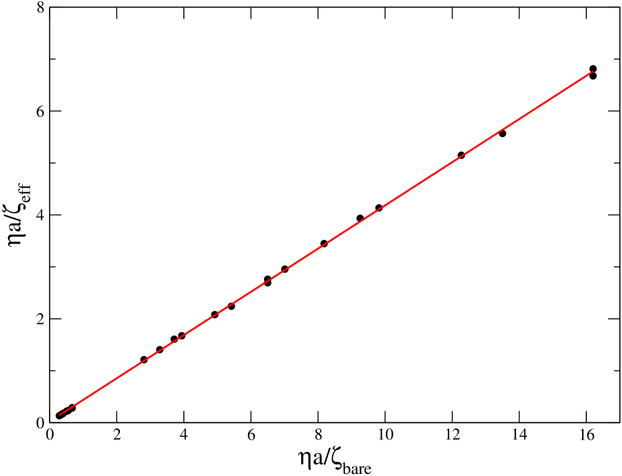
Figure 1:

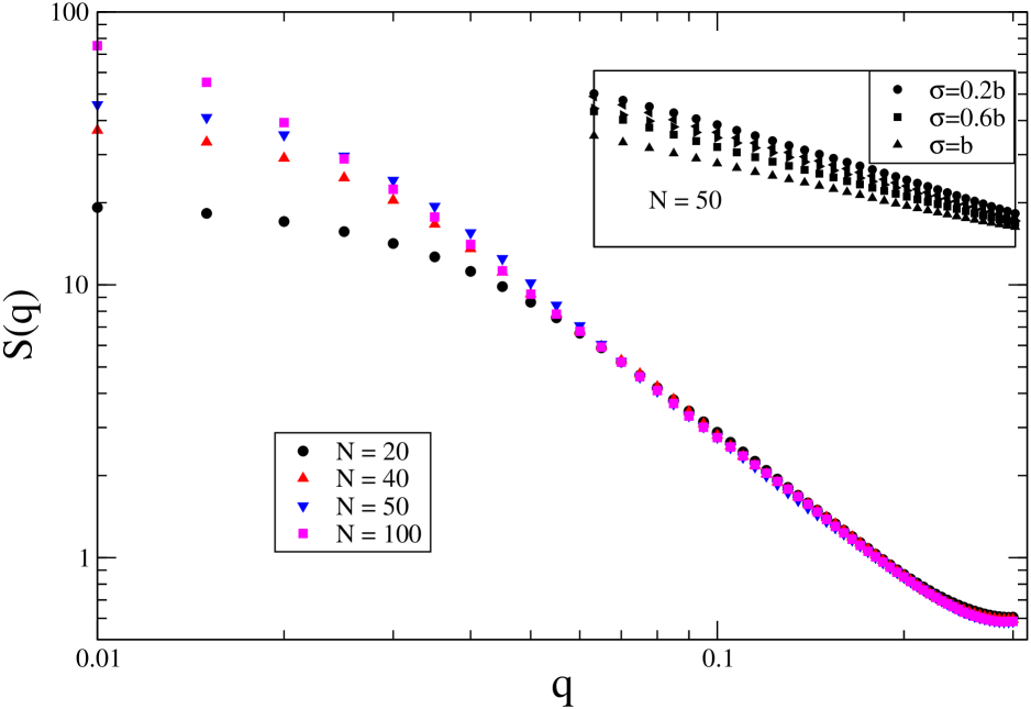
Figure 2:

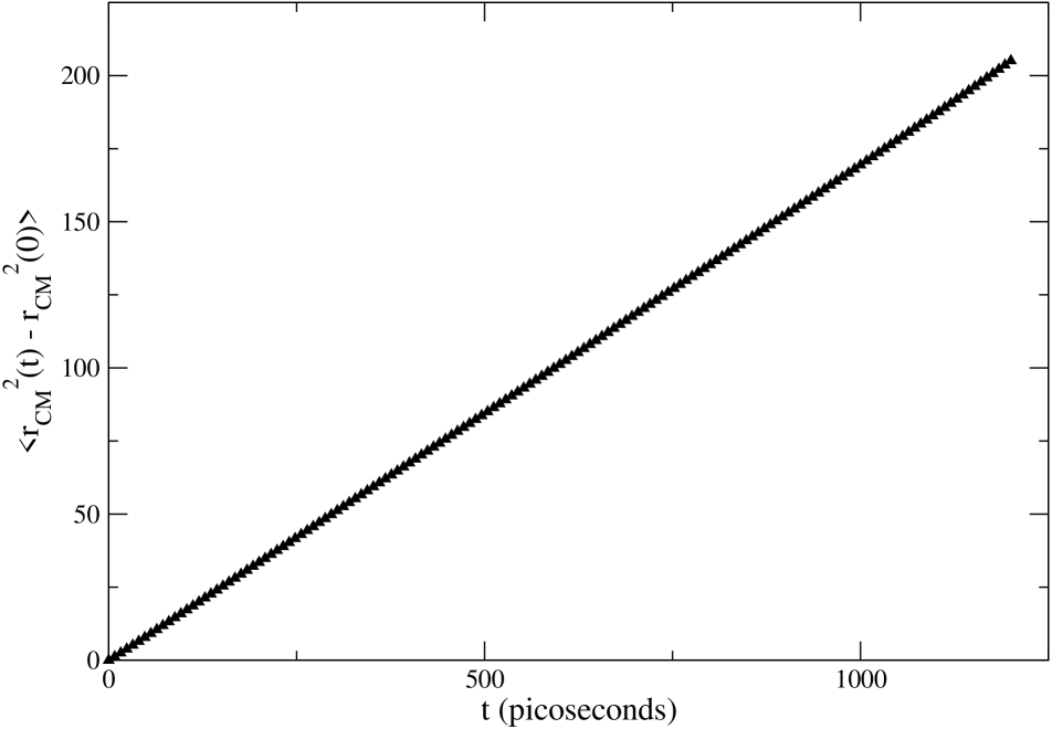
Figure 3:

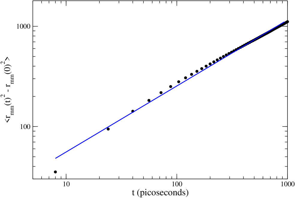
Figure 4:

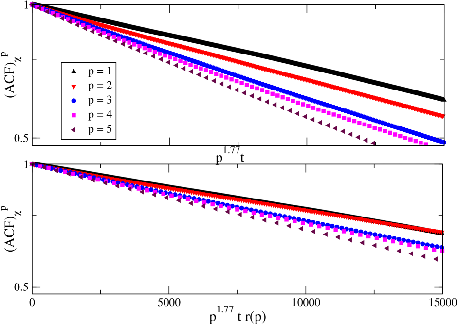
Figure 5:

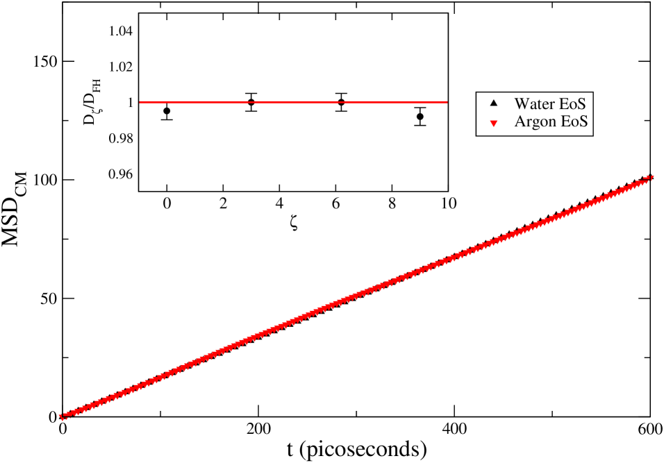
Figure 6:

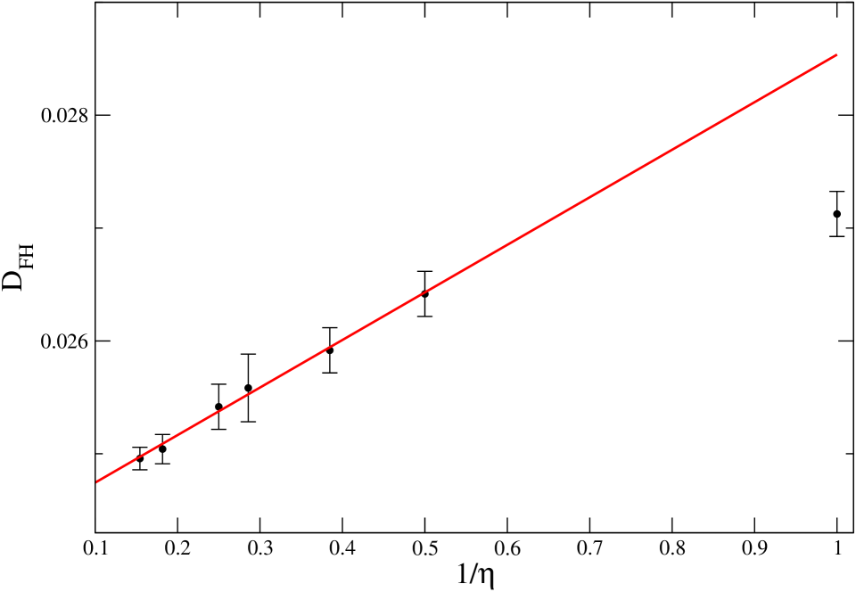
Figure 7:

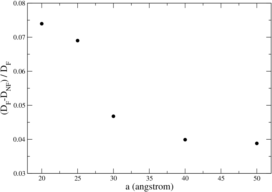
Figure 8:

References

- (1) R. G. Larson, The structure and rheology of complex fluids (Oxford University Press, 1999).
- (2) M. Doi and S. F. Edwards, The theory of polymer dynamics (Clarendon, Oxford, 1995).
- (3) A.J.C. Ladd, Phys. Rev. Lett. 70 1339 (1993).
- (4) N. Sharma and A. Patankar, J. Comp. Phys. 210 466-486 (2004).
- (5) P. Ahlrichs and B. Dünweg, J. Chem. Phys. 111 8225 (1999).
- (6) S. Succi, The lattice Boltzmann equation for fluid dynamics and beyond (Oxford University Press, 2001).
- (7) P. Ahlrichs and B. Dünweg, Int. J. Mod. Phys. C 9 1429 (1998).
- (8) O.B. Usta, A.J.C. Ladd and J.E. Butler, J. Chem. Phys. 122 094902 (2005).
- (9) K. Mussawisade, M. Ripoll, R. G. Winkler and G. Gomper, J. Chem. Phys. 123 144905 (2005).
- (10) J.T. Padding, A.A. Louis, Phys. Rev. E C 74 031402 (2006).
- (11) S.H. Lee and R. Kapral, J. Chem. Phys. 124 214901 (2006).
- (12) J.F. Ryder and J.M. Yeomans, J. Chem. Phys. 125 194906 (2006).
- (13) G. De Fabritiis, M. Serrano, R. Delgado-Buscalioni and P.V. Coveney, Phys. Rev. E 75 026307 (2007).
- (14) G. De Fabritiis, R. Delgado-Buscaglioni and P.V. Coveney, Phys. Rev. Lett. 97 134501 (2006).
- (15) L. D. Landau and E. M. Lifshitz, Fluid mechanics (Pergamon Press, New York, 1959).
- (16) G. Giupponi, G. De Fabritiis and P.V. Coveney, A coupled molecular-continuum hybrid model for the simulation of macromolecular dynamics. Int. J. Mod. Phys. - In press (2007).
- (17) M. P. Allen and D. J. Tildesley Computer simulation of liquids (Oxford University Press, 1989).
- (18) K. Kremer, G.S. Grest, J. Chem. Phys. 92 5057 (1990).
- (19) A. MacKerell, D. Bashford, M. Bellot, R. Dunbrack, J. Evanseck, M. Field, S. Fischer, J. Gao, H. Guo, S. Ha et al. J. Phys. Chem. B 102 3586 (1998).
- (20) E. Pitard, Eur. Phys. J. B 7 665-673 (1999).
- (21) V. Symeonidis, R. G. E. Karniadakis and B. Caswell, Phys. Rev. Lett. 95 076001 (2005).
- (22) G. De Fabritiis, G. Giupponi and P.V. Coveney, An implicit hydrodynamic solvent model: polymer collapse dynamics in poor solvents. preprint (2007).
- (23) M.E. Cates, J.C. Desplat, P. Stansell, A.J. Wagner, K. Stratford, R. Adhikari, I. Pagonabarraga Phil. Trans. R. Soc. A C 363 1833 (2005).
- (24) J.M. Polson and J.P. Gallant, J. Chem. Phys. 124 184905 (2006).
- (25) Robertson R.M., Laib S. and D.E. Smith, Proc. Natl. Acad. Sci. USA 103 7310-7314 (2006).
- (26) P.K. Depa and J.K. Maranas, J. Chem. Phys. 123 094901 (2005).
- (27) M. Fixman, Macromolecules 14 1710-1717 (1981).
- (28) B. Liu and B. Dünweg, J. Chem. Phys. 118 8061 665-673 (2003).