Localized steady-state domain wall oscillators

Abstract

We predict a spatially localized magnetic domain wall oscillator upon the application of an external magnetic field and a DC electric current. The amplitude and frequency of the oscillator can be controlled by the field and/or the current. The resulting oscillator could be used as an effective microwave source for information storage application.

In a spin valve, a DC electric current generates a spin transfer torque which can control or alter the magnetization dynamics of the free layer. Above a critical current density, the spin transfer torque is able to switch the direction of the magnetization, generate spin wave excitations, and more interestingly, create a steady-state precessional motion of the magnetization of the free layer Kiselev . For a ferromagnetic metal, the spin transfer torque results in domain wall motion Yamaguchi ; Parkin , spin wave excitations Ji ; Li , and wall transformation from one type to another Klaui ; He . What is yet to demonstrate is whether a DC current is able to create a spatially localized domain wall oscillator. A well controlled and spatially localized domain wall oscillator is very desirable for applications. For example, the oscillatory magnetic field from the stray fields of a localized domain wall oscillator can assist writing magnetic bits in recording media. Here, we show that a stable and localized domain wall oscillator is indeed possible by the combined applications of the magnetic field and the current. We determine the relevant parameters for this realization.

Domain wall motion driven by a magnetic field has been well studied Schryer ; Malozemoff ; Nakatani ; Beach . When the magnetic field exceeds a critical value, the domain wall overcomes the pinning potential and begins to move to reduce the Zeeman energy. As a first approximation, the domain wall moves uniformly and the velocity of the wall is given by $\gamma H\Delta_{0}/\alpha$ Schryer where $\gamma$ is the gyromagnetic ratio, $H$ is the magnetic field along the wire, $\Delta_{0}$ is the wall width, and $\alpha$ is the damping parameter. When the magnetic field is further increased beyond the Walker-breakdown field, the wall motion is no more uniform; instead, the wall velocity becomes oscillatory Parkin . However, the oscillation can not be sustained because the wall motion or wall oscillation continuously decreases the magnetic energy due to the presence of damping. After a typical time scale of nanoseconds, the domain wall either stops precessing or completely moves out of any finite regions, i.e., a spatially localized wall oscillation driven by a DC magnetic field alone is not realizable.

We show below that the spatially localized wall oscillator is possible when a current is also applied. By properly choosing the direction and magnitude of the current density for a given magnetic field, the average velocity of the wall can be precisely controlled at zero, and thus a stable and spatially localized oscillator can be created. There is a key difference between the field-driven and current-driven domain wall dynamics: the energy damped in a period of wall oscillation can be compensated by the energy input from the spin transfer torque, but no compensation occurs for the magnetic field since the change of the Zeeman energy is zero for a full cycle of oscillation.

To determine the relevant parameters for the creation of the localized wall oscillator, we consider the dynamic equation of the magnetization in the presence of field and current Zhang ; Thiaville ; Bauer ,

$$\frac{\partial{\bf M}}{\partial t} = -\gamma{\bf M}\times{\bf H}_{eff}+\frac{\alpha}{\it{M}_{s}}{{\bf M}}\times\frac{\partial{\bf M}}{\partial t}$$

$$-\frac{b_{J}}{\it{M}^{\bf{2}}_{s}}{{\bf M}}\times\left({{\bf M}}\times\frac{\partial{\bf M}}{\partial x}\right)-\frac{c_{J}}{\it{M}_{s}}\bf{M}\times\frac{\partial\bf{M}}{\partial\it{x}}$$

where ${\bf H}_{eff}$ is the effective magnetic field including the external field, the anisotropy field, the magnetostatic field, and the exchange field; $b_{J}=Pj_{e}\mu_{B}/eM_{s}$ and $c_{J}=\xi b_{J}$, where P is the spin polarization of the current; $j_{e}$ is the current density, $\mu_{B}$ is the Bohr magneton, $e$ is the electron charge, and $M_{s}$ is the saturation magnetization. $\xi$ is a dimensionless constant which describes the degree of the nonadiabaticity between the spin of the non-equilibrium conduction electrons and local magnetization.

We solve above dynamic equation in two ways. First, we analyze a simplified model based on the Walker’s wall profile Schryer : this enables us to analytically determine the condition for the formation of the wall oscillator. Numerical calculations are then followed to verify our analytical results. In Walker’s model, the domain wall structure is characterized by two variables: the center position of the wall $q(t)$ and the angle of the wall plane $\phi(t)$. The wall width $\Delta_{0}$ is treated as a constant. With these simplifications, one can write Eq. (1) in terms of $q(t)$ and $\phi(t)$,

$$\Delta_{0}\dot{\phi}+{\alpha}{\dot{q}} = \gamma\Delta_{0}H-c_{J}$$ (2)

$$\dot{q}-\alpha\Delta_{0}\dot{\phi} = \gamma 2\pi M_{s}\Delta_{0}\sin{2\phi}-b_{J}.$$ (3)

Eliminating $\dot{q}$ from above equations, we have

$$\dot{\phi}=\frac{\gamma}{(1+\alpha^{2})}\left(H_{0}-H_{w}\sin{2\phi}\right)$$ (4)

where we have defined field $H_{0}=H+(\alpha-\xi)b_{J}/(\gamma\Delta_{0})$, and the Walker breakdown field $H_{w}=\alpha 2\pi M_{s}$. When $H_{0}<H_{w}$, Eq.(4) has a steady state solution, i.e., $\dot{\phi}=0$ and $\sin{2\phi}=H_{0}/H_{w}$; this is the solution for the uniform motion of the wall with velocity: $\dot{q}=(\gamma\Delta_{0}H-c_{J})/\alpha$. When $H_{0}>H_{w}$, however, there is no steady-state solution; this is known as the Walker breakdown Schryer . The direct integration of Eq. (4) yields

$$\tan\phi(t)=C_{1}+\sqrt{1-C_{1}^{2}}\tan(\omega t)$$ (5)

where $C_{1}=H_{w}/H_{0}$ and $\omega=\gamma\sqrt{H_{0}^{2}-H_{w}^{2}}/(1+\alpha^{2})$. Equation (5) indicates that the angle $\phi$ increases a $\pi$ in one period $T_{\phi}=\pi/\omega$. Thus the average angular velocity is

$$\dot{\bar{\phi}}=\pi/T_{\phi}=\frac{\gamma}{(1+\alpha^{2})}\sqrt{H_{0}^{2}-H_{w}^{2}}.$$ (6)

By averaging Eq. (2) over one oscillation period and by using Eq. (6), we arrive at the condition for the localized oscillator (setting $\dot{\bar{q}}=0$),

$$b_{J}=\frac{\gamma\Delta_{0}}{\xi}\left(H-\frac{\sqrt{H_{0}^{2}-H_{w}^{2}}}{1+\alpha^{2}}\right).$$ (7)

The amplitude of the oscillation can be obtained by solving for $q$ when $\dot{q}=0$. There are two solutions; their difference (divided by 2) is identified as the oscillation amplitude $q_{amp}$. From Eqs.(2), (3) and (7), we have

$$q_{amp}\simeq\frac{\Delta_{0}H_{w}}{2\alpha H}.$$ (8)

To further gain the insight on the solution of the localized wall oscillation, let us consider the change of wall energy in one period of oscillation. Multiply Eq (2) by $\dot{q}$ and multiply Eq. (3) by $\Delta_{0}\dot{\phi}$, and then substrate the resulting equations from each other, we have

$$\pi\Delta_{0}b_{J}=\alpha\int_{0}^{T_{\phi}}dt(\dot{q}^{2}+\Delta_{0}^{2}\dot{\phi}^{2}).$$ (9)

The right hand side represents the domain wall energy loss in one cycle, which has to be compensated by the work done by the spin torque on the left hand side. Note that the external field does not contribute any work in a complete cycle; this is the physical reason why the field alone is unable to sustain a localized domain wall oscillation.

Up till now, we have considered the solution of localized wall oscillations in an ideally uniform film or wire. The center position of the wall oscillation is arbitrary as long as Eq. (7) is met. Any spatial variation of the parameters would lead to a drift of wall position. In order to stabilize the center of the wall oscillation at a desired location, one needs to design a structure that can suppress the drifting of the wall center but maintain the wall oscillation. At first, one might consider a local pinning to trap the oscillator, for example, by using a higher anisotropy material in a small region. However, we find that such local pinnings are not effective at all. If the pinning is strong, the wall oscillation is completely destroyed and a static domain wall will be formed at the pinning site. If the wall oscillation persists over a weaker pinning potential, the wall center remains unstable against a small fluctuation of parameters. The reason is that the amplitude of the wall oscillation is several times larger than the wall width, see Eq. (8), so that the local pinning does not affect the oscillation significantly. We thus propose a scheme to stabilize the oscillation by designing a spatially varying damping parameter–this can be achieved via gradient doping of rare-earth impurities in ferromagnets Reidy . We argue below that the wall oscillation is spatially stable in this design.

Consider a spatial dependence of the damping parameter $\alpha(q)$. For a fixed current $b_{J}$ and field $H$, the center of the oscillation will be located at a certain position $q=x_{0}$ so that Eq. (7) is satisfied when $\alpha=\alpha(x_{0})$. Then if there is a fluctuation, for example, the current density is slightly increased, the wall center will move along the direction of electron current. The equation of motion for the center of the wall is, from Eqs. (2) and (3),

$$\ddot{\bar{q}}\simeq\gamma\Delta_{0}H_{0}\left[2+\frac{(2\pi M_{s})^{2}}{H_{0}^{2}}\right]\frac{d\alpha}{d\bar{q}}\dot{\bar{q}}$$ (10)

where $H_{w}\ll H_{0}$ and $\alpha\ll 1$ have been used. Clearly, if $d\alpha/d\bar{q}<0$, i.e., the damping parameter increases along the direction of the electron current (note $d\bar{q}<0$ if $b_{J}$ is increased), the drifting velocity of the center of oscillation $\dot{\bar{q}}$ exponentially decays to zero. The wall oscillates around a new position near the original oscillation center, where Eq. (9) is still satisfied on average.

Next we numerically solve Eq. (1) to validate our analytical results. We choose a magnetic wire whose width and thickness are sufficiently small so that the transverse wall is energetically favorable compared to the vortex wall. We also choose $\alpha=\xi=0.02$ throughout the simulation; when $\alpha\neq\xi$, there is no qualitative difference on the behavior of the wall motion except that the effective magnetic field has an additional term given by $(\alpha-\xi)b_{J}/(\gamma\Delta_{0})$. In Fig. 1, we show the typical wall velocity $\dot{\bar{q}}$ as a function of the magnetic field with and without the current. The linearly increasing of $\dot{\bar{q}}$ at small fields represents the uniform steady-state motion of the wall. When $H_{0}>H_{w}$, the average velocity decreases since the domain wall does a reciprocative motion, i.e., the wall motion is oscillatory but $\dot{\bar{q}}$ is generally non-zero – the oscillator is not localized. At certain values of the field and current, we find $\dot{\bar{q}}=0$, indicated by the mark “$\it X$” in Fig. 1. In the insert, we show the oscillation of the wall center position $q(t)$ around a fixed point ($x=0$). We notice that the current density required for the localized oscillator is relatively small, $b_{J}=20m/s$ or $j_{e}=3.9\times 10^{7}A/cm^{2}$ (for $P=0.7$), compared to the experiments on current-driven domain wall motion Parkin ; Yamaguchi ; Hayashi ; Tsoi2 ; this makes experiments of searching for the localized oscillator easily accessible.

We describe the stability of the localized oscillator by choosing a linearly varying damping parameter $\alpha(x)=0.02\times(1-x/L)$, where $L$ is the wire length and $-L/2<x<L/2$. We first consider the field $H$ and the current $b_{J}$ such that the oscillator is localized at $x=0$, see the point “$\it X$” in Fig. 1. When we slightly vary the current density or the magnetic field, the oscillator will relocate to a new center position $x_{1}$ near $x=0$. The time evolution of the displacement $q(t)$ at this new position (not shown) is similar as the insets of Fig. (1). We show in Fig. 2 the position of the wall oscillation center, amplitude and frequency of the localized oscillator for the varying magnetic fields and currents. These results are in good agreements with the analytical results, Eqs. (6), (7), and (8).

Finally, we emphasize that the localized domain wall oscillators proposed here is quite different from the previous work Tatara1 ; Tatara2 where either an AC current or an AC magnetic field is used as a driving force. In those cases, a strong pinning potential via geometrical confinement is used to localize the domain wall and the oscillation of the wall is simply a response to the oscillatory external force (AC fields or currents). Our proposal here is to generate the wall oscillation by a DC magnetic field and to localize the oscillator by a DC electrical current. A spatial varying damping parameter can effectively stabilize the oscillator.

This work is partially supported by DOE and Seagate Technologies Inc.

Figure Caption

FIG.1 (Color online) Average velocity of the domain wall $v=\dot{\bar{q}}$. The parameters are: $M_{s}=800$ (emu/cc), $H_{K}=500$ (Oe), $A=1.3\times 10^{-6}$ (erg/cm). Note we have chosen a reduced Breakdown field similar to the experimental value $H_{w}=9$ (Oe) Hayashi . The fitting curves are the analytical solutions of $\dot{\bar{q}}$ from Eqs. (2) and (6), and the fitted wall width $\Delta_{0}=20$nm. Insets show the time evolution of the displacement $q(t)$ at the point “$\it X$”.

FIG.2 (Color online) Position of the wall oscillation center $x_{1}$, amplitude $q_{amp}$ and frequency $f=\omega/\pi$ of the oscillator as a function of the field and current: (a), (b) and (c) are for a fixed current, and (d), (e) and (f) for a fixed field. Damping parameter is $\alpha(x)=0.02\times(1-x/L)$, where $L=0.8\mu$m.

Figure 1:

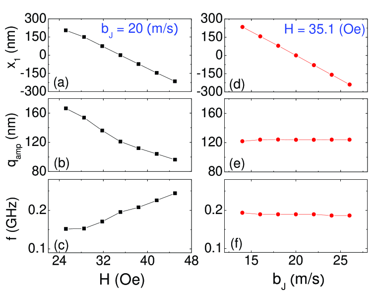
Figure 2:

References

- (1) S. I. Kiselev, J. C. Sankey, I. N. Krivorotov, N. C. Emley, R. J. Schoelkopf, R. A. Buhrman and D. C. Ralph, Nature 425, 380 (2003).
- (2) A. Yamaguchi, T. Ono, S. Nasu, K. Miyake, K. Mibu and T. Shinjo, Phys. Rev. Lett. 92, 077205 (2004).
- (3) M. Hayashi, L. Thomas, C. Rettner, R. Moriya and S. S. P. Parkin, Nature Physics 3, 21-25 (2007).
- (4) Y. Ji, C. L. Chien and M. D. Stiles, Phys. Rev. Lett. 90, 106601 (2003).
- (5) Z. Li and S. Zhang, Phys. Rev. Lett. 92, 207203 (2004).
- (6) M. Klui, P.-O. Jubert, R. Allenspach, A. Bischof, J. A. C. Bland, G. Faini, U. Rdiger, C. A. F. Vaz, L. Vila and C. Vouille, Phys. Rev. Lett. 95, 026601 (2005).
- (7) J. He, Z. Li and S. Zhang, J. Appl. Phys. 99, 08G509 (2006).
- (8) N. L. Schryer and L. R. Walker, J. Appl. Phys. 45, 5406 (1974).
- (9) A. P. Malozemoff, J. C. Slonczewski, Magnetic Domain Walls in Bubble Materials, Academic Press, New York, 1979.
- (10) Y. Nakatani, A. Thiaville and J. Miltat, Nature Materials 2, 521-523 (2003).
- (11) G. S. D. Beach, C. Nistor, C. Knutson, M. Tsoi and J. L. Erskine, Nature Materials 4, 741-744 (2005).
- (12) S. Zhang and Z. Li, Phys. Rev. Lett. 93, 127204 (2004).
- (13) A. Thiaville, Y. Nakatani, J. Miltat and Y. Suzuki, Europhys. Lett., 69 (6), 990-996 (2005).
- (14) Y. Tserkovnyak, H. J. Skadsem, A. Brataas and G. E. W. Bauer, Phys. Rev. B 74, 144405 (2006).
- (15) S. G. Reidy, L. Cheng and W. E. Bailey, Appl. Phys. Lett. 82, 1254 (2003).
- (16) M. Hayashi, L. Thomas, Ya. B. Bazaliy, C. Rettner, R. Moriya, X. Jiang and S. S. P. Parkin, Phys. Rev. Lett. 96, 197207 (2006).
- (17) G. S. D. Beach, C. Knutson, C. Nistor, M. Tsoi and J. L. Erskine, Phys. Rev. Lett. 97, 057203 (2006).
- (18) E. Saitoh, H. Miyajima, T. Yamaoka and G. Tatara, Nature 432, 203-206 (2004).
- (19) G. Tatara, E. Saitoh, M. Ichimura and H. Kohno, Appl. Phys. Lett. 86 232504 (2005).