Two-parameter scaling law of the Anderson transition

Abstract

It is shown that the Anderson transition (AT) in $3d$ obeys a two-parameter scaling law, derived from a pair of anisotropic scaling transformations, and corresponding critical exponents and scaling function calculated, using a high-precision numerical finite-size scaling study of the smallest Lyapunov exponent of quasi-$1d$ systems of rectangular cross-section of $L\times\delta L$ atoms in the limit of infinite $L$ and $\delta L<L$, for $x=\delta L/L$ ranging from $1/30$ to $1/4$. The second parameter is $x$, and there are two singularities: apart from the two-parameter scaling describing AT for $x>0$, corrections to scaling due to the irrelevant scaling field diverge when $x\to 0$, and the corresponding crossover length scale is also estimated. Furthermore, results suggest that the signatures of the AT in $3d$ should be present also in $2d$ strongly localized regime.

One of the long-standing open fundamental problems of the physics of quantum-mechanical disordered systems is the quantitative description of the metal-insulator transition induced by the Anderson localization of electronic eigenstates Anderson58 , known as the Anderson or localization-delocalization transition (AT). The subsequently developed scaling theory of localization of Abrahams et al. Abrahams79 (STL) proposed that: (i) in $3d$ the transition is a continuous phase transition with only one relevant scaling variable (which became known as the single- or one-parameter scaling hypothesis), (ii) the lower critical dimension is $2$ where all states are localized for arbitrarily small finite disorder strength, and (iii) the transition can be described in terms of the scaling law of the disorder-averaged dimensionless conductance $g$ that depends only on $g$, i.e $d\ln g/d\ln L=\beta_{d}(g)$. The theory is based on the renormalization-group (RG) considerations of the Thouless expression for $g$, and an additional calculation showing that $\beta_{d=2}(g)<0$, which was corroborated by a more detailed self-consistent study Vollhardt80 based on a resummation of the perturbation theory for weak disorder Langer66 .

The discovery of the universal conductance fluctuations Lee85 ; Mesoscopic91 showed that $g$ is not a self-averaging quantity, and therefore scaling of its whole distribution has to be studied. The STL nevertheless survived in the sense that one can still find a single parameter $g$ that characterizes scaling properties of the whole distribution, and there is a compelling evidence that the scaling properties of the distribution itself in the critical region of the transition are still governed by a single-parameter Shapiro86 .

Numerical studies of the transition using the transfer-matrix method (TMM) Pichard81 suggested a possibility that $\beta_{d=2}(g)=0$ for a finite amount of disorder, which would correspond to the existence of a line of critical points for disorder weaker than a certain finite disorder strength, but subsequent studies showed that the dependence of localization length on the disorder strength in $2d$ is in a quantitative agreement with analytical results MacKinnon81 ,

High precision numerical calculations of the critical exponent $\nu$ describing the divergence of the localization length $\xi$ at the critical point in $3d$, however, give $\nu\approx 1.54$ MacKinnon94 ; Slevin99 , in sharp contrast with $\nu=1$ obtained from the self-consistent analytical calculations Abrahams79 ; Vollhardt80 .

Theoretical breakthrough was made by Efetov Efetov83 , who introduced supersymmetry to calculate disorder-averaged products of Green’s functions, and provided a theoretical framework that, among other results, allows calculation of $\nu$ beyond the self-consistent approach, although technical difficulties with the $\epsilon$-expansion do not yet permit accurate estimate of $\nu$ despite the considerable theoretical progress Hikami81 , and currently $\nu$ is most accurately determined using TMM.

This Letter present three main results: (1) there is an additional scaling parameter $x$ in $d=3$ describing the thickness to width ratio of long quasi-$1d$ wires, and the corresponding two-parameter scaling law and critical exponents are estimated numerically; (2) results are in agreement with (ii) and additionally show that there should be possible to see signatures of $3d$ transition in $2d$; (3) the description of the transition in terms of the $\beta$-function depending only on $L$ is incomplete due to the geometric nature of both $x$ and $L$.

The starting point is the Anderson model Anderson58 :

$$H=\sum_{i}\epsilon_{i}|i\rangle\langle i|+t\sum_{\langle ij\rangle}(|i\rangle\langle j|+|j\rangle\langle i|),$$ (1)

where $\epsilon_{i}$ represents the impurity energy at site $i$. $\epsilon_{i}$ is randomly, independently and uniformly distributed in $[-W/2,W/2)$; $t$ is the hopping integral of electron (set to 1), $\langle ij\rangle$ denotes that the hopping takes place only between the nearest-neighbors of the simple cubic lattice, and the Fermi energy is set to 0 (band center).

The geometry studied is that of the quasi-$1d$ slabs of $L\times\delta L\times M$ atoms with $M\gg L$, ratio $x=\delta L/L$, open boundary conditions (b.c) in $\delta L$ direction and periodic b.c in $L$ direction. Similar geometry of cubic samples of $L_{0}\times L_{0}\times(qL_{0})$ atoms was studied in Ref. Potempa98 , where authors found that the critical disorder strength $W_{c}$ is approx. independent of the shape and that $g$ becomes strongly suppressed for $q\ll 1$ and $q\gg 1$ which is consistent with, respectively, the quasi-$2d$ and quasi-$1d$ character of samples in these cases.

The scaling properties of AT in $3d$ are studied by the standard calculation of the smallest Lyapunov exponent $\gamma$ of transfer matrices of long quasi-$1d$ samples MacKinnon94 ; Slevin99 . The inverse of $\gamma$ is the largest length scale in the problem, which is identified with the correlation length $\xi=1/\gamma$. The usually studied quantity is the rescaled correlation length $\Lambda$ defined as $\Lambda(L,W)\equiv(L\gamma(L,W))^{-1}$

The finite-size scaling analysis of $\Lambda$ gives the scaling properties of $3d$ systems in the thermodynamic $L\to\infty$ limit, by considering how $\Lambda(L,W)$ changes under the RG transformation $\mathcal{R}:L\mapsto b^{\prime}L,\delta L\mapsto b^{\prime}L$ Cardy96 . The corresponding scaling law, including the corrections to scaling due to one irrelevant field was considered in the context of AT first by Slevin and Othsuki Slevin99 , who were able to numerically show that

$$\Lambda(L,w)=F(L^{1\over{\nu}}\psi(w),L^{y}\phi(w)),\;w=\frac{W-W_{c}}{W_{c}},$$ (2)

where $\nu>0$ and $y<0$ are critical exponents associated with, respectively, the relevant and irrelevant scaling fields $\psi$ and $\phi$, and all functions are analytic. This is achieved by fitting numerically obtained values of $\Lambda$ with the truncated expansions of $F,\phi,$ and $\psi$, while the error-bars are estimated via calculation of $95\%$ confidence intervals that can be done either by the bootstrapping method Slevin99 or by a direct calculation of projections of the confidence region Cerovski07b .

In the case when there is an additional parameter $x$, we can repeated the above procedure for several values of $x$,

$$\Lambda(L,w,x)=F(L^{1\over{\nu}}\psi(w,x),L^{y}\phi(w,x),x),$$ (3)

where $\nu,y,W_{c}$ may in general also depend on $x$. The principal difference between Eq. (2) and Eq. (3) is that $F,\psi$ and $\phi$ do not have to be necessarily analytic in $x$.

Expansion in the second argument of $F$ gives:

$$\bar{\Lambda}(L,w,x) = F_{\pm}(L^{1\over\nu}\psi(w,x),x),\;\bar{\Lambda}=\Lambda-\Delta F,$$ (4)

$$\Delta F = \sum_{n=1}^{\infty}F_{n}(L^{1\over\nu}\psi(w,x),x)\phi(w,x)^{n}L^{ny},$$ (5)

where $F_{\pm}$ represents the universal part describing AT, and $\Delta F$ are corrections to scaling due to $\phi$. These vanish for large $L$ because $y<0$ but are important for a quantitative description of AT, including precise determination of all of the relevant parameters Slevin99 ; Cerovski07b .

$x$	$\delta L$	$W$	$N_{d}$	$N_{p}$	$\chi^{2}$	$Q$	$W_{c}$	$\nu$	$y$
$1$	$[4,14]$	$[15,18]$	$427$	$10$	$439.1$	$0.2$	$16.46(39,55)$	$1.60(55,65)$	$-1.39(1.16,1.62)$
$3/4$	$[3,15]$	$[15,18]$	$304$	$10$	$282.4$	$0.7$	$16.52(46,60)$	$1.62(57,66)$	$-1.13(0.98,1.29)$
$1/3$	$[1,4]$	$[15,18]$	$427$	$10$	$418.2$	$0.5$	$16.52(42,63)$	$1.54(48,61)$	$-1.00(0.90,1.10)$
$1/4$	$[1,7]$	$[15,18]$	$427$	$10$	$436.9$	$0.2$	$16.48(42,54)$	$1.55(51,60)$	$-1.00(0.97,1.04)$
$1/7$	$[1,5]$	$[14.25,18]$	$380$	$11$	$370.0$	$0.5$	$16.61(47,77)$	$1.52(39,67)$	$-0.89(0.84,0.95)$
$1/10$	$[1,6]$	$[14.5,18]$	$370$	$11$	$365.7$	$0.4$	$16.62(50,75)$	$1.52(41,66)$	$-0.88(0.84,0.93)$
$1/15$	$[1,4]$	$[14.5,18.25]$	$304$	$11$	$298.2$	$0.4$	$16.58(23,95)$	$1.62(41,87)$	$-0.90(0.80,0.99)$
$1/20$	$[1,4]$	$[14.5,18.25]$	$304$	$11$	$287.3$	$0.6$	$16.59(27,99)$	$1.57(37,89)$	$-0.90(0.80,1.00)$
$1/30$	$[1,4]$	$[14.5,18.5]$	$324$	$11$	$350.3$	$0.1$	$16.50(27,80)$	$1.59(51,69)$	$-0.93(0.85,1.01)$

Table 1: Input parameters of the simulation: $x$, thickness $\delta L$, the number of points $N_{d}$, the number of parameters $N_{p}$; Output values: the minimal least-square deviation $\chi^{2}$ obtained, the quality of fit parameter $Q$; and the values of the fitting parameters: the critical disorder strength $W_{c}$, the critical exponent $\nu$ and the irrelevant exponent $y$. All $\Lambda$’s are calculated with $0.1\%$ relative accuracy except for the largest systems studied ($x=1/30,\delta L=4$), which is calculated with accuracy of $0.12\%$. Error-bars are $95\%$ confidence intervals.

Figure 1 shows the typical behavior of $\Lambda(L,W)$ and the corresponding fit for small constant $x$ and several $\delta L$ starting with 1. As $L=\delta L/x$ increases, $\Lambda(L,W)$ at first decreases uniformly in $W$ (since for small $\delta L$ system is close to being $2d$) but with further increase of $L$ a characteristic behavior for the continuous transition begins to develop, since for large $\delta L$ and constant $x$ system is $3d$.

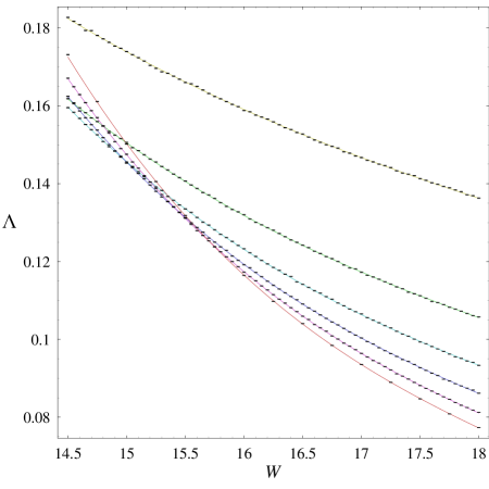
Figure 1: Values of $\Lambda(L,W)$ for $x=1/10$. The corresponding fits are represented with lines for $\delta L=1,...,6$ (going from the slowest changing curve to the fastest).

Table 1 summarizes the parameters and the results of the numerical simulation using the methods described above for several values of $x$. Results presented in the Table suggest that $\nu$ is approx. independent of $x$ and in agreement with Ref. MacKinnon94 ; Slevin99 ; Cerovski07b , which supports its universality. Similar can be said for $W_{c}$, in agreement with Ref. Potempa98 , while $y$ becomes approx. constant for $x\lessapprox 1/4$.

To better understand the scaling properties of AT w.r.t $x$, I consider an additional scaling transformation, $\mathcal{R}_{x}:x\mapsto bx$ under constant $L$ (this is equivalent to scaling only the thickness $\delta L$), and introduce a scaling field $\tilde{\psi}$ that depends on $x$ but not on $w$:

$$\bar{\Lambda}=F_{\pm}(L^{1\over\nu}\psi(w,x),\tilde{\psi}(x)),$$ (6)

where $W_{c},\nu$ and $y$ are assumed to be constant. The scaling law of $F_{\pm}$ w.r.t $x$ can be derived assuming that functions scale under $\mathcal{R}_{x}$ in the general way Cardy96 :

$$\mathcal{R}_{x}:F_{\pm}\mapsto b^{y_{1}}F_{\pm},\;\psi\mapsto b^{y_{2}}\psi,\;\tilde{\psi}\mapsto b^{y_{3}}\tilde{\psi},$$ (7)

Iterating $\mathcal{R}_{x}$ a finite number of times in the standard manner gives the two-parameter scaling law:

$$\bar{\Lambda}=x^{\alpha}\mathcal{F}_{\pm}(L^{1\over\nu}x^{\mu}\psi(w)),$$ (8)

where $\alpha\equiv-y_{1}/y_{3},\mu\equiv-y_{2}/y_{3}$.

At first it seems that Eq. (8) cannot be correct in the case of AT for small $x$ because numerical results give that the transition takes place at approx. const. $W_{c}$, and if $W_{c}$ would remain constant for smaller $x$ as well, Eq. (8) would imply that transition persists when $x\to 0$ (regardless of the value of $\alpha$), where one must find strongly localized states instead.

This is resolved if we notice that $\Delta F$ is also divergent as $x\to 0$, and that there is a characteristic crossover length-scale $L_{c}(x)$ such that for $L\gtrsim L_{c}(x)$ corrections to scaling become small, but $L_{c}(x)\to\infty$ when $x\to 0$. The source of the divergence for $W\approx W_{c}$ is in $\phi(x,w=0)=\phi_{0}(x)$, and the left panel of Fig. 2 shows that $\phi(x)\propto x^{\delta}$ for $x\lessapprox 1/7$, with $\delta=-0.17(05,29)$. $L_{c}(x)$ is determined from the condition $L_{c}(x)^{y}\phi(x)\sim 1$, giving

$$L_{c}(x)\sim x^{-{\delta\over y}}.$$ (9)

A more detailed discussion of the exponent $\delta$ will be carried out elsewhere since our main interest here is in the two-parameter scaling law Eq. (8) of AT.

$\alpha$ is calculated from the dependence of $\Lambda_{c}$ on $x$, where $\Lambda_{c}=\bar{\Lambda}(W=W_{c})$. The right panel of Fig. 2 shows that $\alpha=0.89(84,95)$. Numerical verification of Eq. (8) is done by a rescaling of the argument of $\bar{\Lambda}/\Lambda_{c}$ for each $x$ individually by a factor $\theta(x)$ chosen such that all $\bar{\Lambda}/\Lambda_{c}$ collapse, and Fig. 3 shows the result. Figure 4 shows that $\theta(x)\propto x^{\mu_{1}},\mu_{1}=2.75(2.28,3.16)$ and $\psi(x)\propto x^{\mu_{2}},\mu_{2}=1.34(22,46)$, which gives $\mu=\mu_{1}+\mu_{2}=4.1\pm 0.6$.

Figure 2: Dependence of $\phi_{0}(x)$ (left panel) and $\Lambda_{c}(x)$ (right panel) on $x$. The solid line in both panels is the least-square linear fit. Error-bars are $95\%$ confidence intervals.

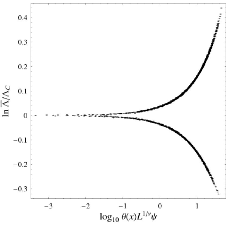
Figure 3: Collapse of $\bar{\Lambda}(L,W,x)$ onto the universal function $\mathcal{F}_{\pm}$, for 2109 points from Table 1 corresponding to $x\leq 1/4$.

Figure 4: Dependence of the rescaling factor $\theta(x)$ (left panel) and the relevant scaling field $\psi$ (right panel) on $x$. The solid line in both panels is the least-square linear fit. Error-bars in the right panel are $95\%$ confidence intervals.

The largest similarity with the one-parameter scaling Eq. (2) is achieved for $\alpha=1,\,\mu=1/\nu$, when Eq. (8), expressed in terms of $\xi$, becomes

$$\xi(L,w,x)\simeq(xL)\mathcal{F}_{\pm}((xL)^{1\over\nu}\psi(w)).$$ (10)

$x$ influences the divergence of the correlation length of the infinite system $\xi_{\infty}(w,x)\sim(|w|/x)^{-{1\over\nu}}$ for $L\gtrsim L_{c}(x)$. The numerical results are not incompatible with $\alpha=1$, but nonetheless strongly suggest $\mu\neq\alpha/\nu$.

The two-parameter scaling was obtained for samples of small $\delta L$, including the single-layered case (Table 1). This allows one to follow outflow RG trajectories from $L\to\infty$ back to the single-layered finite $L$ case, and therefore provides an analytical mapping of the phase diagram of $3d$ systems onto $2d$ systems, suggesting a possibility of signatures of $3d$ AT also in $2d$ strongly-localized regime. What exactly those signature are, including a possibility of their experimental observation in the mesoscopic regime, will be discussed elsewhere Cerovski07c .

Although the study carried here shows the possibility of AT in arbitrarily thin $3d$ films (which should be of size $L\gtrsim L_{c}(x)$ in order to reduce the large corrections to scaling due to the dimensional crossover) in the strong-disorder regime, the critical conductance is strongly suppressed due to the $x^{\alpha}$ prefactor.

The RG approach proposed seems to be a rather accurate description of AT and allows the nontrivial extension of the one-parameter STL to two parameters. It remains to be seen whether such an approach can be applicable to other problems in physics, for instance in addition to the dimensional regularization.

References

- (1) P. W. Anderson, Phys. Rev. 109, 1492 (1958).
- (2) E. Abrahams, P. W. Anderson, D. C. Licciardello and T. V. Ramakrishnan, Phys. Rev. Lett. 42, 673 (1979).
- (3) D. Vollhardt and P. Wölfle, Phys. Rev. Lett. 45, 842 (1980); Phys. Rev. B 22, 4666 (1980).
- (4) J. S. Langer and T. Neal, Phys. Rev. Lett. 16, 984 (1966).
- (5) P. A. Lee and A. D. Stone, Phys. Rev. Lett. 55, 1622 (1985).
- (6) B. L. Altshuler, P. A. Lee, and R. A. Webb, eds., Mesoscopic Phenomena in Solids (North-Holland, Amsterdam, 1991).
- (7) B. Shapiro, Phys. Rev. B 34, 4394 (1986); Philos. Mag. B 56, 1031 (1987); B. L. Altshuler, V. E. Kravtsov, and I. V. Lerner, Phys. Lett. A 134, 488 (1989); B. Shapiro, Phys. Rev. Lett. 65, 1510 (1990); K. Slevin, P. Markoš, and T. Ohtsuki, Phys. Rev. Lett. 86, 3594 (2001); Phys. Rev. B 67, 155106 (2003); K. Slevin, Y. Asada, and L. I. Deych, Phys. Rev. B 70, 054201 (2004).
- (8) J. L. Pichard and G. Sarma, J. Phys. C 34, L127 (1981).
- (9) A. MacKinnon and B. Kramer, Phys. Rev. Lett. 47, 1546 (1981); Z. Phys. B: Condens. Matter 53, 1 (1983).
- (10) A. MacKinnon, J. Phys.: Condens. Matter 6, 2511 (1994).
- (11) K. Slevin and T. Ohtsuki, Phys. Rev. Lett. 82, 382 (1999).
- (12) K. B. Efetov, Adv. Phys. 32, 53 (1983).
- (13) S. Hikami, Phys. Rev. B 24, 2671 (1981); V. E. Kravtsov, I. V. Lerner, and V. I. Yudson, Sov. Phys. JETP 67, 1441 (1988). F. Wegner, Nucl. Phys. B 316, 663 (1989); Z. Phys. B: Condens. Matter 78, 33 (1990); E. Breźin and S. Hikami, Phys. Rev. B 55, R10169 (1992); S. Hikami, Prog. Theor. Phys. Suppl. 107, 213 (1992).
- (14) H. Potempa and L. Schweitzer, J. Phys. Condens. Matter 10, L431 (1998).
- (15) J. Cardy, Scaling and Renormalization in Statistical Physics (Cambridge University Press, Cambridge, 1996).
- (16) V. Z. Cerovski, to appear in Phys. Rev. B, preprint No. cond-mat/0701306 (2007).
- (17) V. Z. Cerovski, (unpublished) (2007).