Precise asymptotics for a variable-range hopping model

Abstract

For a system of localised electron states the DC conductivity vanishes at zero temperature, but localised electrons can conduct at finite temperature. Mott gave a theory for the low-temperature conductivity in terms of a variable-range hopping model, which is hard to analyse. Here we give precise asymptotic results for a modified variable-range hopping model, proposed by S. Alexander [Phys. Rev. B, 26, 2956 (1982)].

1 Introduction

If a system has localised electron states the DC conductivity must be zero at zero temperature, but localised electrons can conduct at finite temperatures. Mott [1] proposed that the low-temperature dependence of the DC conductivity is

$$\sigma(T)\sim\exp\Big{[}-\Big{(}\frac{T_{0}}{T}\Big{)}^{\frac{1}{d+1}}\Big{]}$$ (1)

in $d$ spatial dimensions (variable-range hopping law).

The variable-range hopping process is described by specifying transition rates for an electron to hop from one localised site to another. The standard model is illustrated in one spatial dimension in figure 1. It is of the form of a resistor network, with nodes labelled by $n=1,\ldots,N$. The conductances $\Gamma_{nm}$ are given by the transition rates

$$\Gamma_{nm}=\Gamma_{0}\,\exp\left(-\frac{\displaystyle|E_{n}|+|E_{m}|+|E_{n}-E_{m}|}{\displaystyle 2k_{\rm B}T}\right)\,\epsilon^{\displaystyle|n-m|}$$ (2)

where $E_{m}$ are random on-site energies (measured relative to the Fermi energy). Here the exponential factor accounts for the temperature dependence of the rate constants and the factor $\epsilon^{|n-m|}$ models the decrease of the matrix elements as a function of distance between the sites. The matrix elements are assumed to decrease exponentially as a function of hopping distance, with parameter $\epsilon\equiv\exp(-\alpha)$ (where $\alpha$ is the inverse localisation length). In the low-temperature limit the rate constants differ by orders of magnitude, so that the conduction of the chain is determined by a single path, and the conductivity is the harmonic mean of the dominant transition rates. Transitions have a higher rate if they require a small increase in the energy of the electron, which favours finding a conduction path involving low-energy states. There is thus a competition between hopping to a nearby site, which is favoured by large transition matrix elements, and finding an energetically favoured site, which may be some distance away.

Despite the appealing simplicity of this physical picture, there are no precise asymptotic expressions and few significant results on variable-range hopping. Ambegaokar et al. [2] have employed the fact that the transition rates between localised electron states in disordered solids fluctuate wildly to map the variable-range hopping problem onto a percolation problem. This explains the exponent in (1) for $d>1$ and provides an estimate of $T_{0}$. Kurkijärvi [3] showed that the DC conductivity in infinitely long disordered chains is simple activated conduction, following the Arrhenius law: $\sigma(T)\sim\exp(-T_{0}/T)$. This result was later refined by Raikh and Ruzin [4]. In one dimension, Mott’s law (1) is expected to be valid for sufficiently short chains only.

Alexander [5] introduced a simplified model for variable-range hopping. In this paper we discuss the physical significance of his model and analyse it using an alternative method. We obtain a precise asymptotic expression for the conductivity according to this model.

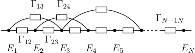
Figure 1: One-dimensional resistor-network model for a one-dimensional variable-range hopping problem. The conductances $\Gamma_{nm}$ are given by (2), $E_{n}$ are random on-site energies.

2 The Alexander model

Finding the true conduction path is a difficult problem. Here, following Ref. [5], we adopt a simpler approach. We construct a conduction path, visiting a sequence of sites by the following scheme. Given the $i$th site in the sequence, at position $n$ in the lattice, we take the site $i+1$ to be the site with position $m$ which has the largest transition rate $\Gamma_{nm}$ [given by equation (2)], considering only sites lying to the right. (That is, we maximise $\Gamma_{nm}$ with respect to $m$, subject to $m>n$). This approach will not usually produce the optimal conduction path, for which a non-optimal transition at one step may be more than compensated by a lower overall resistance. However, the model has the appealing feature that its asymptotics can be determined precisely, as we now show.

We can simplify the model further by assuming that the rate is $\Gamma_{nm}=\epsilon^{|n-m|-\omega_{n}/t}$, where $\omega_{n}$ is a random number and $t$ a small parameter. In the following we assume that the $\omega_{n}$ are independently, identically uniformly distributed in $[0,1]$.

3 Method of solution

Because the values of $\Gamma_{nm}$ differ by orders of magnitude we can approximate the largest rate $\Gamma$ from a given site to some other site by the sum over all rates

$$\Gamma=\sum_{n=0}^{\infty}\epsilon^{n}x_{n}$$ (3)

where $x_{n}={\rm e}^{-\omega_{n}/t}$. The probability density for the random variables $x_{n}$ is

$$\rho(x)=\left\{\begin{array}[]{ll}t/x&\mbox{for}\,\quad\exp(-t^{-1})\leq x\leq 1\\ 0&\mbox{otherwise.}\end{array}\right.$$ (4)

The conductivity of the system is obtained from the diffusion constant $D$, which is given by $D=-J\Delta N/\Delta p$, where $\Delta p$ is the change in occupation probability over $\Delta N$ sites. We have $\Delta p=J\sum_{i}\Gamma_{i}^{-1}=J\langle\Gamma^{-1}\rangle\Delta N_{\rm step}$, where $\Delta N_{\rm step}$ is the number of maximum-rate hops in the process described above. If the maximum-rate hops have average length $\langle\Delta n\rangle$, then $\Delta N_{\rm step}=\Delta N/\langle\Delta n\rangle$, and the diffusion constant is

$$D=\langle\Gamma^{-1}\rangle^{-1}\,\langle\Delta n\rangle\ .$$ (5)

The quantity $\langle\Delta n\rangle$ may be determined by considering

$$\epsilon{\partial\log\Gamma\over{\partial\epsilon}}={\sum_{n}n\epsilon^{n}x_{n}\over{\sum_{n}\epsilon^{n}x_{n}}}\,.$$ (6)

This will almost always be approximately equal to the value of $n$ for which the rate $\epsilon^{n}x_{n}$ is maximal. Thus we may write

$$\langle\Delta n\rangle=\epsilon{\partial\over{\partial\epsilon}}\langle\log\Gamma\rangle$$ (7)

and we have the ingredients necessary to determine $D$ from the probability density $\rho_{\Gamma}$ of $\Gamma$.

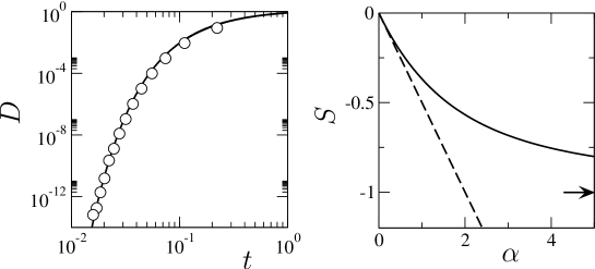
Figure 2: (Left) shows results of numerical simulations for diffusion constant $D$ as a function of $t$ ($\circ$) for $\epsilon=0.2$, compared to the exact asymptotic theory, equation (29). (Right) shows $S(\alpha)$, equation (30), as a function of $\alpha$ (solid line). Also shown is the approximate result $S(\alpha)\sim-\alpha/2$ from Ref. [5] (dashed line). The arrow indicates the nearest-neighbour limit $S=-1$.

4 Distribution of $\Gamma$

The distribution of $\Gamma$ may be obtained from $\rho(x)$ [the distribution of the variables $x_{n}$ in (3)], by application of the convolution theorem. Because $\Gamma$ is a sum of independent random variables, its probability density is the convolution of the probability density of each component, namely $\rho(x/\epsilon^{n})$. Correspondingly, the generalised Fourier transform $\tilde{\rho}_{\Gamma}(k)$ of the required probability density is a product:

$$\tilde{\rho}_{\Gamma}(k)=\prod_{n=0}^{\infty}\tilde{\rho}(k\epsilon^{n})$$ (8)

where the generalised Fourier transform is defined by

$$\tilde{\rho}(k)=\int_{-\infty}^{\infty}\!\!{\rm d}x\ \exp({\rm i}kx)\rho(x)\,.$$ (9)

Setting $u=kx$ we obtain

$$\tilde{\rho}(k) = t\int_{\raisebox{-8.53581pt}{$\scriptstyle k\exp(-1/t)$}}^{k}{\rm d}u\ u^{-1}\exp({\rm i}u)$$

$$= t\bigl{[}E_{1}(-{\rm i}k\exp(-1/t)-E_{1}(-{\rm i}k)\bigr{]}$$

where $E_{1}(v)$ is the exponential integral

$$E_{1}(v)=\int_{x}^{\infty}{\rm d}z\ {\exp(-z)\over z}\,.$$ (11)

From the asymptotic form for $E_{1}(v)$ we find $\tilde{\rho}(0)=1$ (which is required by normalisation). Further we find $|\tilde{\rho}(k)|<t$ for $k>\exp(1/t)$, and that for $1\ll k\ll\exp(1/t)$ we can apply the following approximation:

$$\tilde{\rho}(k)\sim 1-t\log k-\gamma t+\tfrac{1}{2}{\rm i}\pi t\,.$$ (12)

We now determine $\tilde{\rho}_{\Gamma}(k)$. In the case where $|k|\ll 1$ all of the factors are close to unity such that $\tilde{\rho}_{\Gamma}(k)\sim 1$ in that region. In the case where $|k|\gg\exp(1/t)$, the product is negligible, and we approximate $\tilde{\rho}_{\Gamma}(k)\sim 0$ in that region. Finally, when $1\ll k\ll\exp(1/t)$, most of the factors in the infinite product are very close to unity, and we can replace the infinite sum by a finite number $N^{\ast}$ of terms. This number is determined by the value $N^{\ast}$ of the index such that the argument of the corresponding term, $\epsilon^{N^{\ast}}k$ is equal to unity. Thus $N^{\ast}$ is the integer part ${\log k}/{\log(1/\epsilon)}={\log k}/{\alpha}$ and we have

$$\tilde{\rho}_{\Gamma}(k)\sim\prod_{n=0}^{{\rm Int}[(\log k)/\alpha]}\big{(}1-t\log\epsilon^{n}k-\gamma t+\tfrac{1}{2}\pi{\rm i}t\big{)}\,.$$ (13)

Evaluating the product we obtain an approximate expression for $\tilde{\rho}_{\Gamma}(k)$, valid for $t\ll 1$ and $1\ll k\ll\exp(1/t)$:

$$\tilde{\rho}_{\Gamma}(k) \sim (\alpha t)^{1+\alpha^{-1}\log k}\,\,\frac{\Gamma\displaystyle\Big{(}\frac{1+\alpha t-\gamma t+{\rm i}\pi t/2}{\alpha t}\Big{)}}{\Gamma\displaystyle\Big{(}\frac{1-t\log k-\gamma t+{\rm i}\pi t/2}{\alpha t}\Big{)}}\,.$$ (14)

We need to determine the asymptotic form for small values of $t$. Note that $x=\log k$ varies between $0$ and $t^{-1}$ so that $xt$ is of order unity. Using

$$\Gamma(z+a)\sim\sqrt{2\pi}\,{\rm e}^{-z}z^{-\frac{1}{2}+z+a}$$ (15)

for large $z$ and taking $z=(1-xt)/(\alpha t)$, we obtain

$$\tilde{\rho}_{\Gamma}(k) = {\rm e}^{\displaystyle-\frac{x}{\alpha}+\big{(}\frac{1}{2}-\frac{1-xt}{\alpha t}+\frac{\gamma}{\alpha}-\frac{{\rm i}\pi}{2\alpha}\big{)}\log(1-xt)}\,.$$

The calculation of $D$ requires two averages: $\langle\Gamma^{-1}\rangle$ and $\langle\log\Gamma\rangle$. Averages can be calculated in terms of the generalised Fourier transform of the probability density:

$$\langle f(\Gamma)\rangle=\int_{-\infty}^{\infty}{\rm d}\Gamma\ \rho(\Gamma)f(\Gamma)=\frac{1}{2\pi}\int_{-\infty}^{\infty}{\rm d}k\ \tilde{\rho}_{\Gamma}(k)\tilde{f}(k)$$ (17)

where $\tilde{f}(k)$ is the generalised Fourier transform of the weight function $f(\Gamma)$.

5 Harmonic average of $\Gamma$

We have

$$\langle\Gamma^{-1}\rangle=\int_{0}^{\infty}{\rm d}k\ \mbox{Im}[\tilde{\rho}_{\Gamma}(k)]$$ (18)

since the generalised Fourier transform of $1/\Gamma$ is $\pi{\rm i}\,\mbox{sgn}(k)$. We evaluate the integral in the saddle-point approximation. To this end let $y=xt=t\log k$. Note that the contribution to integrals with respect to $k$ from the interval $[0,1]$ is negligible and is not considered. We thus have

$$\langle\Gamma^{-1}\rangle\sim\frac{1}{t}\int_{0}^{1}\!{\rm d}y\,{\rm e}^{t^{-1}S(y)}{\rm e}^{(\frac{1}{2}+\frac{\gamma}{\alpha})\log(1-y)}\sin\phi(y)$$ (19)

with

$$S(y) = y-\frac{y}{\alpha}-\frac{1-y}{\alpha}\log(1-y)\,,$$ (20)

$$\phi(y) = \frac{\pi}{2\alpha}\log(1-y)\,.$$

The saddle-point equations are:

$$y^{\ast} = 1-{\rm e}^{-\alpha}\,,$$ (21)

$$S(y^{\ast}) = \frac{-1+\alpha+{\rm e}^{-\alpha}}{\alpha}\,,$$

$$\phi(y^{\ast}) = -\frac{\pi}{2}\,,$$

$$\frac{\partial^{2}S^{\ast}}{\partial y^{2}} = -\frac{{\rm e}^{\alpha}}{\alpha}\,.$$

It follows that

$$\langle\Gamma^{-1}\rangle\sim\sqrt{\frac{2\pi\alpha}{t}}\,{\rm e}^{\displaystyle-\alpha-\gamma}\,{\rm e}^{\displaystyle\frac{-1+\alpha+{\rm e}^{-\alpha}}{\alpha t}}\,.$$ (22)

6 Average of $\log\Gamma$

To calculate $\langle\log\Gamma\rangle$, we make use of the relation

$$\langle\log\Gamma\rangle=\frac{2}{\pi}\int_{0}^{\infty}{\rm d}k\ {\log|k|+\gamma\over k}\mbox{Im}[\tilde{\rho}_{\Gamma}(k)]\,.$$ (23)

From equation (23) we find

$$\langle\log\Gamma\rangle \sim \frac{1}{t^{2}}\frac{2}{\pi}\int_{0}^{1}\!\!\!{\rm d}y\,(y+\gamma t)\,{\rm e}^{(\alpha t)^{-1}R(y)}{\rm e}^{(\frac{1}{2}+\frac{\gamma}{\alpha})\log(1-y)}\sin\phi(y)\,.$$ (24)

with

$$R(y) = -y-(1-y)\log(1-y)$$ (25)

and $\phi$ as defined in (20). The integral is approximately

$$\langle\log\Gamma\rangle\sim-\frac{1}{t^{2}}\frac{2}{\pi}\frac{\pi}{2\alpha}\int_{0}^{1}\!\!\!{\rm d}y\,y(y+\gamma t)\,{\rm e}^{(\alpha t)^{-1}R(y)}\,.$$ (26)

Approximating $R(y)=-y^{2}/2$, we obtain

$$\langle\log\Gamma\rangle\sim-(\pi/2)^{1/2}(\alpha/t)^{1/2}\,.$$ (27)

7 Results

Using (7) it follows that

$$\langle\Delta n\rangle\sim\frac{1}{4}\sqrt{\frac{2\pi}{\alpha t}}\,.$$ (28)

Taking equations (5), (22), and (28) together we finally obtain:

$$D\sim\frac{1}{4\alpha}{\rm e}^{\alpha+\gamma}{\rm e}^{[1-\alpha-\exp(-\alpha)]/(\alpha t)}\,.$$ (29)

This is the main result of this paper. It describes the exact asymptotics of the diffusion constant in Alexander’s model, exhibiting Arrhenius behaviour, with action (excitation energy) given by

$$S(\alpha)=\frac{1-\alpha-\exp(-\alpha)}{\alpha}$$ (30)

which is plotted in Fig. 2. The limit $S(0)=-\alpha/2$ (dashed line in Fig. 2) was previously obtained in Ref. [5]. In the opposite limit ($\alpha\rightarrow\infty$) the action converges to $-1$, describing activated transport in a conventional nearest-neighbour model.

In addition to the precise form (30) of the action, our result (29) also gives the pre-exponential prefactor exactly. We know of no variable-range hopping model for which the pre-exponential factor has been obtained precisely. The precise asymptotic expression for $D$ allows for comparison with computer simulations. The simulations were performed as follows: we sampled the rate $\Gamma$ for the optimal hop from a given point to the right, as well as the corresponding length $\Delta n$. The diffusion constant was then calculated from (5). In figure 2, equation (29) is shown together with results of computer simulations for $\epsilon=0.2$ (corresponding to $\alpha\approx 1.62$). We observe excellent agreement between the simulations and the precise asymptotic theory.

Acknowledgements. BM acknowledges financial support from Vetenskapsrådet.

References

- [1] N. F. Mott, J. Non-Cryst. Solids, 1, 1, (1968).
- [2] V. Ambegaokar, B. I. Halperin, and J. S. Langer, Phys. Rev. B, 4, 2612 (1971).
- [3] J. Kurkijärvi, Phys. Rev. B, 8, 622, (1973).
- [4] M. E. Raikh and I. M. Ruzin, Sov. Phys. JETP, 66, 642-7, (1989) [Zh. Eksp. Teor. Fiz., 95, 1113-22, (1989).]
- [5] S. Alexander, Phys. Rev. B, 26, 2956 (1982).