Contact lines for fluid surface adhesion

Abstract

When a fluid surface adheres to a substrate, the location of the contact line adjusts in order to minimize the overall energy. This adhesion balance implies boundary conditions which depend on the characteristic surface deformation energies. We develop a general geometrical framework within which these conditions can be systematically derived. We treat both adhesion to a rigid substrate as well as adhesion between two fluid surfaces, and illustrate our general results for several important Hamiltonians involving both curvature and curvature gradients. Some of these have previously been studied using very different techniques, others are to our knowledge new. What becomes clear in our approach is that, except for capillary phenomena, these boundary conditions are not the manifestation of a local force balance, even if the concept of surface stress is properly generalized. Hamiltonians containing higher order surface derivatives are not just sensitive to boundary translations but also notice changes in slope or even curvature. Both the necessity and the functional form of the corresponding additional contributions follow readily from our treatment.

I Introduction

There exist a number of physical systems whose energetics is fully described by a surface Hamiltonian. The easiest and best known examples involve capillary phenomena RowlinsonWidom ; deGennesBrochardQuere , where the shape of a liquid-fluid interface (such as a sessile water droplet or the shape of a fluid meniscus) is determined by minimizing its area. The same physics governs the behavior of soap films. Higher order surface properties, notably its curvature, play a role in the description of fluid lipid membranes or microemulsions Canham70 ; Helfrich73 , and even higher derivatives have been implicated in the occurrence of certain corrugated membrane phases GoeHel96 . In all these cases the shape of the surface follows from minimizing the surface Hamiltonian, a variational problem. The corresponding Euler-Lagrange differential equations are known as the shape equations.

However, such surfaces are generally not isolated but rather in contact with something else. Water droplets or lipid membrane vesicles may rest on a substrate, and this generally influences their shape quite strongly. For instance, water droplets on hydrophilic substrates (e. g. clean glass) resemble flat contact lenses, while on very hydrophobic substrates (e. g. teflon) they are almost completely spherical. When gravity can be neglected gravity , the shape equation dictates a constant mean curvature surface in both cases (in fact, a spherical cap), but the contact angle at the three-phase line where water and substrate meet is different for the two different substrates.

In the majority of cases the spatial extension of the surface being studied exceeds the range of interaction between it and some substrate by a large amount. For instance, van der Waals forces, hydrophobic interactions, or (screened) electrostatic forces typically extend over several nanometers, while the extensions of vesicles or droplets can be microns or even millimeters. Under these conditions the interaction is well approximated by a contact energy, i. e., an energy per unit area, $w$, liberated when the surface makes contact with the substrate. It is this adhesion energy, together with the energy parameters characterizing the contacting surfaces, which determines the boundary conditions holding at the contact line. In the case of capillary phenomena for example the ratio between adhesion energy $w$ and surface tension $\sigma$ determines the contact angle $\vartheta$ between liquid and substrate surface by means of the well-known Young-Dupré equation RowlinsonWidom ; deGennesBrochardQuere

$$\frac{w}{\sigma}=1+\cos\vartheta\ .$$ (1)

The “standard” derivation of this result involves a balance of tangential forces at the contact line. Yet, despite being very intuitive, this requirement of surface stress balance does not yield the correct condition for more complicated surface Hamiltonians, even if the concept of surface stress is generalized properly. Higher order Hamiltonians give rise to additional energy contributions when the contact line is varied. It is the purpose of the present article to show how these contributions can be accounted for in a systematic and parametrization-free way, and without assuming any additional symmetries (such as axisymmetry or translation symmetry along the contact line). We study adhesion to rigid substrates as well as to deformable surfaces also characterized by a surface Hamiltonian. Our presentation generalizes and strongly simplifies the analysis previously given in Ref. CapovillaGuven_adhesion .

II Mathematical setup

II.1 Differential geometry

In order to describe the adhering surfaces in a parametrization-free way, we use a covariant differential geometric language. Our notation is essentially standard and will follow the one used in Refs. CapovillaGuven_adhesion ; surfacestresstensor ; auxiliary ; mem_inter_short ; mem_inter_long . Briefly, a surface $\mathcal{S}$ is described by the embedding function ${\boldsymbol{X}}(\xi^{1},\xi^{2})\in\mathbb{R}^{3}$, where the $\xi^{a}$ $(a\in\{1,2\})$ are a suitable set of local coordinates on the surface. This induces two local tangent vectors ${\boldsymbol{e}}_{a}=\partial{\boldsymbol{X}}/\partial\xi^{a}=\partial_{a}{\boldsymbol{X}}$ and a normal vector satisfying ${\boldsymbol{n}}\cdot{\boldsymbol{e}}_{a}=0$ and ${\boldsymbol{n}}^{2}=1$. Furthermore, the two fundamental forms of the surface are needed, namely ($i$) the metric tensor $g_{ab}={\boldsymbol{e}}_{a}\cdot{\boldsymbol{e}}_{b}$ and ($ii$) the extrinsic curvature tensor $K_{ab}={\boldsymbol{e}}_{a}\cdot\nabla_{b}{\boldsymbol{n}}=-{\boldsymbol{n}}\cdot\nabla_{a}{\boldsymbol{e}}_{b}$. The symbol $\nabla_{a}$ is the metric-compatible covariant derivative. The trace of the extrinsic curvature tensor will be denoted by $K=K_{a}^{a}=K_{ab}g^{ab}$, which for a sphere of radius $r$ with outward pointing normal vector is positive and has the value $K=2/r$. As usual, indices are lowered or raised with the metric or its inverse, respectively, and a repeated index $i$ (one up, one down) implies a summation over $i=1,2$. More background on differential geometry can be found in Refs. doCarmo ; Spivak ; Kreyszig .

II.2 Geometry at the contact line

By “contact line” we will denote the curve $\mathcal{C}$ at which the surface detaches from the substrate. Its local direction is given by the tangent vector ${\boldsymbol{t}}=t^{a}{\boldsymbol{e}}_{a}$ (see Fig. 1), which is tangential to $\mathcal{C}$, the surface $\mathcal{S}$, and the substrate surface $\underline{\mathcal{S}}$ (which itself might also be deformable). Here and in what follows (with the exception of Sec. IV.2) we will use underlining in order to indicate quantities referring to the substrate.

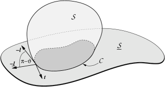
Figure 1: Illustration of the geometry of surface adhesion. Perpendicular to the contact line $\mathcal{C}$ two vectors exist, ${\boldsymbol{l}}$ and $\underline{{\boldsymbol{l}}}$, which are tangential to surface $\mathcal{S}$ and substrate $\underline{\mathcal{S}}$, respectively.

Perpendicular to $\mathcal{C}$ we can define local normal vectors which are either tangential to $\mathcal{S}$ or $\underline{\mathcal{S}}$, namely ${\boldsymbol{l}}=l^{a}{\boldsymbol{e}}_{a}$ and $\underline{{\boldsymbol{l}}}=\underline{l}^{a}\underline{{\boldsymbol{e}}}_{a}$, respectively (see Fig. 1). Also, we will have two surface normals ${\boldsymbol{n}}$ and $\underline{{\boldsymbol{n}}}$. If the surface contacts the substrate at zero contact angle, we will have ${\boldsymbol{e}}_{a}=\underline{{\boldsymbol{e}}}_{a}$, ${\boldsymbol{n}}=\underline{{\boldsymbol{n}}}$, and ${\boldsymbol{l}}=\underline{{\boldsymbol{l}}}$ there; however, their derivatives perpendicular to the contact line need not coincide, since the curvatures of surface and substrate generally need not be identical. In fact, the values of perpendicular and parallel components of these curvatures (and possibly their higher derivatives) will be among the primary focus of this paper. They will be denoted by

$$K_{\perp} \;=\; l^{a}l^{b}K_{ab} \;=\;-{\boldsymbol{n}}\cdot\nabla_{\perp}{\boldsymbol{l}}\ ,$$ (2a)

$$K_{||} \;=\; t^{a}t^{b}K_{ab} \;=\;-{\boldsymbol{n}}\cdot\nabla_{||}{\boldsymbol{t}}\ ,$$ (2b)

$$K_{\perp||}\,=\,K_{||\perp} \;=\; l^{a}t^{b}K_{ab} \;=\;-{\boldsymbol{n}}\cdot\nabla_{\perp}{\boldsymbol{t}}\,=\,-{\boldsymbol{n}}\cdot\nabla_{||}{\boldsymbol{l}}\ ,$$ (2c)

where we also introduced the two directional surface derivatives perpendicular and parallel to $\mathcal{C}$,

$$\nabla_{\perp}=l^{a}\nabla_{a}\qquad\text{and}\qquad\nabla_{||}=t^{a}\nabla_{a}\ .$$ (3)

Notice that we can analogously define $\underline{K}_{\perp}$, $\underline{K}_{||}$, and $\underline{K}_{\perp||}$.

II.3 Hamiltonian

In the present work we will exclusively study surfaces whose energy $H$ is given by a surface integral over a scalar energy density $\mathcal{H}$, which is constructed from the local surface geometry:

$$H=\int_{\mathcal{S}}{\operatorname{d}}A\;\mathcal{H}(g_{ab},K_{ab},\nabla_{a}K_{bc},\ldots)\ .$$ (4)

The integral extends over the entire surface $\mathcal{S}$, and the area element ${\operatorname{d}}A$ is given by $\sqrt{g}\,{\operatorname{d}}\xi^{1}{\operatorname{d}}\xi^{2}$, where $g=\det(g_{ab})$ is the metric determinant. For those parts of the surface which adhere to a substrate we will assume an additional adhesion energy density

$$\mathcal{H}_{\text{adhesion}}=-w(\xi^{1},\xi^{2})\leq 0\ ,$$ (5)

which may in general be a function of position.

III Determining the boundary conditions

III.1 Continuity considerations

As we will see, the adhesion balance between surface and substrate will result in a discontinuous change of some surface property across the contact line. However, the form of the energy density restricts which quantities can be discontinuous, since it needs to remain integrable.

Most obviously, the shape itself has to be continuous. Yet, already its first derivative may display a jump, as it does in the case of capillary adhesion. The energy density is given simply by

$$\mathcal{H}_{\text{capillary}}=\sigma\ ,$$ (6)

and a kink in the surface at the contact line, i. e. a finite contact angle, is not associated with an extra energy.

For curvature elastic surfaces the situation is different. There, the energy density of the surface is given by the well known expression Canham70 ; Helfrich73

$$\mathcal{H}_{\text{bend}}=\frac{1}{2}\kappa(K-K_{0})^{2}\ ,$$ (7)

where $\kappa$ is the bending modulus (with units of energy) and $K_{0}$ describes a spontaneous curvature of the elastic surface GaussBonnet . A kink in the surface at the contact line implies a $\delta$-singularity in the curvature, whose square is non-integrable. Hence, the surface needs to be differentiable across the contact line, and the distinction between surface- and substrate tangents and normals drawn in Sec. II.2 becomes unnecessary. Moreover, a quick glance at Eqns. (2b,2c) shows that both $K_{||}$ and the off-diagonal curvature $K_{\perp||}$ is expressible as a tangential derivative along the curve $\mathcal{C}$ of a quantity continuous across $\mathcal{C}$, hence both these curvatures will also be continuous. It is only the perpendicular curvature component $K_{\perp}$ which might possess a discontinuity, and indeed we will see that it does.

Finally, even higher order derivatives might occur in surface Hamiltonians. For instance, Goetz and Helfrich have studied a curvature-gradient term of the form

$$\mathcal{H}_{\text{grad}}=\frac{1}{2}\kappa_{\nabla}(\nabla_{a}K)(\nabla^{a}K)\equiv\frac{1}{2}\kappa_{\nabla}(\nabla K)^{2}\ ,$$ (8)

which in a generalized higher-curvature Hamiltonian prevents the occurrence of infinitely sharp curvature changes GoeHel96 . In this case it is obvious that all curvature components have to be continuous along the substrate, since otherwise again a squared $\delta$-singularity results. Moreover, most of the first order directional derivatives are automatically continuous: The parallel ones, $\nabla_{||}$, again differentiate quantities along $\mathcal{C}$ which are continuous across $\mathcal{C}$ and thus are itself continuous. For the perpendicular ones it turns out that $\nabla_{\perp}K_{||}$ and $\nabla_{\perp}K_{\perp||}$ are continuous, while $\nabla_{\perp}K_{\perp}$ is not. This is intuitively reasonable, since every term involving a “$||$” features at least one less derivative across the contact line and thus cannot jump. A rigorous proof is however a bit more involved. One may for instance proceed like this: Start with the contracted Codazzi-Mainardi equation doCarmo ; Spivak ; Kreyszig $\nabla_{a}K^{ab}-\nabla^{b}K=0$ and project onto $l_{b}$. By decomposing the resulting identity into the local $({\boldsymbol{l}},{\boldsymbol{t}})$ frame, it can be cast in the form

$$\nabla_{\perp}K_{||}=\nabla_{||}K_{\perp||}+(K_{\perp}-K_{||}){\boldsymbol{t}}\cdot\nabla_{||}{\boldsymbol{l}}+2K_{\perp||}{\boldsymbol{l}}\cdot\nabla_{\perp}{\boldsymbol{t}}\ .$$ (9)

Since every term on the right hand side is continuous across $\mathcal{C}$ (recall that derivatives of tangent vectors are essentially curvatures), $\nabla_{\perp}K_{||}$ must be continuous as well. By projecting the contracted Codazzi-Mainardi equation on $t_{b}$ instead, one can show continuity for $\nabla_{\perp}K_{\perp||}$.

III.2 Contact line variation

For an adhering surface the total energy is stationary with respect to variations of the contact line along the substrate. Such a variation contributes twofold to the Hamiltonian: Assume that locally the contact line is moved such that a bit of surface unbinds from the substrate. This removes its corresponding binding energy, as well as any elastic energy associated with the constraint of conforming to the substrate, and thus gives rise to an energy change $\delta H_{\text{bound}}$. On the other hand, the unbound part of the surface acquires at the contact line a new boundary strip which implies also a change $\delta H_{\text{free}}$ in its elastic energy. The boundary condition at the contact line then follows from the stationarity condition

$$\delta H_{\text{cl}}=\delta H_{\text{bound}}+\delta H_{\text{free}}=0\ .$$ (10)

In the case of adhesion to a rigid substrate the bound contribution involves the variation along a surface of known shape. The corresponding term is thus conceptually very different from a deformable substrate or even the free variation, because in both these cases the local shape of the surface is not known. Below we will see how these differences manifest themselves when computing the boundary terms.

III.2.1 The bound variation

For definiteness, let the normal $\underline{{\boldsymbol{l}}}$ to the contact line $\mathcal{C}$ be directed towards the adhering portion of the surface (see Fig. 1). A local infinitesimal normal displacement $\varepsilon$ of the contact line along a rigid substrate thus implies the following obvious change in the bound part of the surface:

$$\delta H_{\text{bound}}=-\int_{\mathcal{C}}{\operatorname{d}}s\;\big{(}\underline{\mathcal{H}}-w\big{)}\varepsilon(s)\ .$$ (11)

The underlining of $\mathcal{H}$ should again indicate that it is evaluated with geometric surface scalars (such as for instance curvatures) pertaining to the substrate. If the substrate is flexible, the $w$ term remains, but the change in elastic energy will instead be taken care of by an additional free boundary variation.

III.2.2 The free variation

The change in energy due to the addition or removal of unbound parts to the boundaries of the surface is identical to the boundary terms in the variation of the free surface. In Ref. auxiliary it has been shown that for Hamiltonians up to curvature order these terms are given by en_ne

$$\delta H_{\text{free}}=-\int_{\mathcal{C}}{\operatorname{d}}s\;l_{a}\Big{[}{\boldsymbol{f}}^{a}\cdot\delta{\boldsymbol{X}}+\mathcal{H}^{ab}{\boldsymbol{n}}\cdot\delta{\boldsymbol{e}}_{b}\Big{]}\ .$$ (12)

Here, ${\boldsymbol{f}}^{a}$ is the surface stress tensor, given by

$${\boldsymbol{f}}^{a}=(T^{ab}-\mathcal{H}^{ac}K_{c}^{b}){\boldsymbol{e}}_{b}-(\nabla_{b}\mathcal{H}^{ab}){\boldsymbol{n}}\ ,$$ (13)

and we have also defined

$$\mathcal{H}^{ab} = \frac{\delta\mathcal{H}}{\delta K_{ab}}\quad\text{and}$$ (14a)

$$T^{ab} = -\frac{2}{\sqrt{g}}\frac{\delta(\sqrt{g}\mathcal{H})}{\delta g_{ab}}\ .$$ (14b)

Finally, $\delta{\boldsymbol{X}}$ and $\delta{\boldsymbol{e}}_{b}$ denote the change of contact line position and the associated change in the slope of the tangent vectors, respectively. Notice that the latter term is only relevant if $\mathcal{H}^{ab}\neq 0$.

IV Specific examples

In this section we will illustrate the above formalism by applying it to several important situations and surface Hamiltonians. In Sec. IV.1 we first treat the problem of adhesion to a rigid substrate. We will see how known results (the Young-Dupré equation and the contact curvature condition for Helfrich-membranes) follow with remarkable ease and can be extended just as quickly to new Hamiltonians. In Sec. IV.2 we look at the boundary conditions involving adhesion to deformable substrates. Specifically, in IV.2.1 we look at the triple line between three tension surfaces, and in IV.2.2 we study the adhesion of two vesicles.

A central ingredient in all this will be the knowledge of the two tensors $\mathcal{H}^{ab}$ and $T^{ab}$ defined in Eqns. (14a,14b). While their determination is not particularly involved, these calculations have been performed previously by us surfacestresstensor ; auxiliary ; mem_inter_short ; mem_inter_long and we will thus simply reuse the results here.

IV.1 Adhesion to a rigid substrate

Since the variation of the contact line has to proceed along the substrate, we must have

$$\delta{\boldsymbol{X}}=\varepsilon\,\underline{{\boldsymbol{l}}}\ .$$ (15)

No component in ${\boldsymbol{t}}$ direction is necessary, since for fluid surfaces this would merely amount to a reparametrization of $\mathcal{C}$. Notice that (15) is nothing but the Lie derivative of ${\boldsymbol{X}}$ along the substrate, since $\mathcal{L}_{\varepsilon\underline{{\boldsymbol{l}}}}{\boldsymbol{X}}=\varepsilon\underline{l}^{a}\nabla_{a}{\boldsymbol{X}}=\varepsilon\underline{l}^{a}\underline{{\boldsymbol{e}}}_{a}=\varepsilon\,\underline{{\boldsymbol{l}}}$. This property holds generally, and we will make use of it later.

The normal component of the change in the surface tangent vectors ${\boldsymbol{e}}_{b}$ only contributes if $\mathcal{H}^{ab}\neq 0$, i. e., if curvature terms enter the Hamiltonian. We will assume that they do it in such a way that differentiability of the surfaces is implied (see Sec. III.1), so that no distinction needs to be drawn between normal and tangent vectors of substrate and adhering surface. We then find

$${\boldsymbol{n}}\cdot\delta{\boldsymbol{e}}_{b}={\boldsymbol{n}}\cdot\nabla_{b}\delta{\boldsymbol{X}}=\varepsilon l^{c}{\boldsymbol{n}}\cdot\nabla_{b}\underline{{\boldsymbol{e}}}_{c}=-\varepsilon l^{c}\underline{K}_{bc}\ ,$$ (16)

where in the last step the equation of Weingarten doCarmo ; Spivak ; Kreyszig has been used; this is again the Lie derivative along the substrate Lie_again . Notice that there still remains a distinction between curvatures of substrate and surface; hence, the derivative of the tangent vectors resulting from a variation along the substrate yields the substrate curvature and not the free surface curvature.

IV.1.1 Capillary surfaces

In this case the energy density is given by Eqn. (6), and as we have seen in Sec. III.1, we will expect a discontinuity in slope at $\mathcal{C}$. The bound variation is

$$\delta H_{\text{bound}}=-\int_{\mathcal{C}}{\operatorname{d}}s\;(\sigma-w)\varepsilon(s)\ .$$ (17)

For this Hamiltonian we have surfacestresstensor ; auxiliary ; mem_inter_short ; mem_inter_long $\mathcal{H}^{ab}=0$ and ${\boldsymbol{f}}^{a}=-\sigma g^{ab}{\boldsymbol{e}}_{b}=-\sigma{\boldsymbol{e}}^{a}$, and therefore

$$l_{a}{\boldsymbol{f}}^{a}\cdot\delta{\boldsymbol{X}}=-\sigma l_{a}{\boldsymbol{e}}^{a}\cdot\varepsilon\underline{{\boldsymbol{l}}}=-\sigma\varepsilon{\boldsymbol{l}}\cdot\underline{{\boldsymbol{l}}}=-\sigma\varepsilon\cos(\pi-\vartheta)\ ,$$ (18)

where $\vartheta$ is the angle between capillary surface and substrate – in other words, the contact angle (see Fig. 1). Equation (10) thus specializes to

$$\delta H_{\text{cl}}=-\int_{\mathcal{C}}{\operatorname{d}}s\;\big{[}\sigma-w+\sigma\cos\vartheta\big{]}\,\varepsilon(s)\ .$$ (19)

Since $\varepsilon(s)$ is arbitrary, the term in square brackets must vanish – which gives the Young-Dupré equation (1).

IV.1.2 Helfrich Hamiltonian

Let us now look at the energy density (7) which describes the continuum behavior of (tensionless) fluid lipid bilayers. In this case $\mathcal{H}^{ab}=\kappa(K-K_{0})g^{ab}$ and for the stress tensor we have surfacestresstensor ; auxiliary ; mem_inter_short ; mem_inter_long

$$l_{a}{\boldsymbol{f}}^{a}\cdot{\boldsymbol{l}}=-\frac{1}{2}\kappa(K-K_{0})^{2}+\kappa(K-K_{0})K_{\perp}\ .$$ (20)

Together with the expressions for the contact line position and tangent variation from Eqns. (15,16) we find

$$\delta H_{\text{cl}} = -\int_{\mathcal{C}}{\operatorname{d}}s\;\bigg{\{}\frac{1}{2}\kappa(\underline{K}-K_{0})^{2}-w$$ (21a)

$$\qquad\qquad-\frac{1}{2}\kappa(K-K_{0})^{2}+\kappa(K-K_{0})K_{\perp}$$

$$\qquad\qquad-\kappa(K-K_{0})\underline{K}_{\perp}\bigg{\}}\;\varepsilon(s)$$

$$= -\int_{\mathcal{C}}{\operatorname{d}}s\;\bigg{\{}\frac{1}{2}\kappa(K_{\perp}-\underline{K}_{\perp})^{2}-w\bigg{\}}\;\varepsilon(s)\ ,$$ (21b)

where in the second step we made use of the continuity condition $K_{||}=\underline{K}_{||}$ discussed in Sec. III.1. Equation (21b) implies a discontinuity in the perpendicular curvature $K_{\perp}$ as the appropriate adhesion boundary condition:

$$K_{\perp}-\underline{K}_{\perp}\;=\;\sqrt{\frac{2w}{\kappa}}\ .$$ (22)

The correct sign after taking the square root follows from the fact that the detaching surface must not penetrate the substrate; unfortunately this depends on ones specific choice of the surface normal vectors.

Quite remarkably, this boundary condition depends neither on the spontaneous curvature $K_{0}$, nor on the local parallel curvature $K_{||}$. It would also remain unaffected if the bilayer were under a finite tension $\sigma$. Formally, it is easily seen to cancel; physically, the reason is that the jump we would expect from the Young-Dupré equation (1) cannot materialize since the curvature terms in the energy density enforce differentiability of the profile at $\mathcal{C}$.

Equation (22) coincides with the result given previously in Ref. CapovillaGuven_adhesion . Its axisymmetric version was first quoted in Ref. Seifert90 , and its specialization to a straight contact line can be found in Ref. LaLi_elast . We want to stress that the $\mathcal{H}^{ab}{\boldsymbol{n}}\cdot\delta{\boldsymbol{e}}_{b}$ term in Eqn. (12), which is responsible for the third line in Eqn. (21a), was crucial in obtaining equation (22). Leaving it out – i. e., only treating the problem as a stress balance – will not result in the correct boundary condition. The only exception (treated via stress-balance in Ref. CapovillaGuven_adhesion ) is the special case of a flat substrate, in which case $\delta{\boldsymbol{e}}_{b}\equiv 0$ and the missing contribution vanishes anyway.

IV.1.3 General Hamiltonians involving $K$

The analysis in the previous section readily extends to Hamiltonians which are expressible in terms of the total extrinsic curvature, $\mathcal{H}=\mathcal{H}(K)$. One finds $\mathcal{H}^{ab}=\mathcal{H}^{\prime}g^{ab}$, where the prime denotes differentiation with respect to $K$, and the tangential stress tensor contribution is

$$l_{a}{\boldsymbol{f}}^{a}\cdot{\boldsymbol{l}}=-\mathcal{H}+\mathcal{H}^{\prime}K_{\perp}\ .$$ (23)

The remarkably simple general boundary condition then reads continuity

$$(\underline{\mathcal{H}}-\mathcal{H})-\mathcal{H}^{\prime}(\underline{K}_{\perp}-K_{\perp})\;=\;w\ .$$ (24)

Notice that unlike the form it takes for the quadratic Hamiltonian discussed in Sec. IV.1.2, this condition generally involves the parallel curvature $K_{||}$ on the contact line.

IV.1.4 Curvature gradients

Finally, we want to study surfaces described by the Hamiltonian density (8), i. e., involving curvature gradients. From earlier work mem_inter_short ; mem_inter_long we know that

$$\mathcal{H}^{ab} = -\kappa_{\nabla}(\Delta K)g^{ab}\qquad\text{and}$$ (25a)

$$l_{a}{\boldsymbol{f}}^{a}\cdot{\boldsymbol{l}} = \kappa_{\nabla}\Big{[}(\nabla_{\perp}K)^{2}-\frac{1}{2}(\nabla K)^{2}-K_{\perp}\Delta K\Big{]}\ .\;\;\;\;$$ (25b)

However, simplemindedly inserting these expressions into the formulas we have used so far does not give the correct result. Here is why: When calculating $\mathcal{H}^{ab}$ and $T^{ab}$ to obtain Eqns. (25), we varied the Hamiltonian (8) with respect to $K_{ab}$ and $g_{ab}$, respectively, and identified the bulk terms (see Sec. 4 in the Appendix of Ref. mem_inter_long ). These variations also leave boundary terms, since the curvature $K=g^{ab}K_{ab}$ appears differentiated. For the purpose of identifying $\mathcal{H}^{ab}$ and $T^{ab}$ they are irrelevant, but they evidently matter now that we are interested in the total energy change upon displacing the boundary. Moreover, the auxiliary framework introduced in Ref. auxiliary teaches us that the $\delta K_{ab}$ and $\delta g_{ab}$ variations are indeed independent from the $\delta{\boldsymbol{X}}$ and $\delta{\boldsymbol{e}}_{a}$ terms already included in Eqn. (12), so they can be simply added there. If we go through the calculation, we see that the two tensor variations can be nicely combined into a single scalar one, since they occur in the combination $g^{ab}\delta K_{ab}+K_{ab}\delta g^{ab}=\delta K$, and we end up with the additional boundary contribution

$$\delta H_{\text{free,grad}}=\kappa_{\nabla}\int_{\mathcal{C}}{\operatorname{d}}s\;l_{a}(\nabla^{a}K)\delta K\ .$$ (26)

This is of course exactly the boundary term we would expect for the variation of a Hamiltonian density whose functional form is the square of the gradient of a scalar, so everything is consistent.

To evaluate the right hand side of Eqn. (26), note that the variation is once more given by the Lie-derivative along the substrate. Since $K$ is a scalar, we obtain the simple expression

$$\delta K=\mathcal{L}_{\varepsilon{\boldsymbol{l}}}K=\varepsilon l^{a}\nabla_{a}\underline{K}=\varepsilon\nabla_{\perp}\underline{K}\ .$$ (27)

Together with Eqns. (25) we then obtain the total contact line variation as

$$\delta H_{\text{cl}} = -\int_{\mathcal{C}}{\operatorname{d}}s\;\bigg{\{}\frac{1}{2}\kappa_{\nabla}(\nabla\underline{K})^{2}-w$$ (28a)

$$\qquad\qquad+\kappa_{\nabla}\Big{[}(\nabla_{\perp}K)^{2}-\frac{1}{2}(\nabla K)^{2}-K_{\perp}\Delta K\Big{]}$$

$$\qquad\qquad+\kappa_{\nabla}(\Delta K)\underline{K}_{\perp}$$

$$\qquad\qquad-\kappa_{\nabla}(\nabla_{\perp}K)(\nabla_{\perp}\underline{K})\bigg{\}}\;\varepsilon(s)$$

$$= -\int_{\mathcal{C}}{\operatorname{d}}s\;\bigg{\{}\frac{1}{2}\kappa_{\nabla}(\nabla_{\perp}K_{\perp}-\nabla_{\perp}\underline{K}_{\perp})^{2}-w\bigg{\}}\;\varepsilon(s)\ ,$$ (28b)

where in the last step we used the continuity of curvatures and their $\nabla_{||}$-derivatives (as discussed in Sec. III.1) as well as the decomposition $(\nabla K)^{2}=(\nabla_{\perp}K)^{2}+(\nabla_{||}K)^{2}$. The boundary condition following from this specifies a jump in the perpendicular derivative of the perpendicular curvature

$$\nabla_{\perp}\big{(}K_{\perp}-\underline{K}_{\perp}\big{)}\;=\;\sqrt{\frac{2w}{\kappa_{\nabla}}}\ .$$ (29)

The similarity with Eqn. (22) is quite striking, and one might surmise a pattern that would be followed by even higher derivative theories. Notice, however, that the terms entering the derivation of Eqn. (29) are quite different and that the additional term stemming from Eqn. (26), which is absent in the simple curvature square case, is essential.

IV.2 Adhesion to deformable surfaces

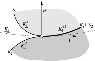
Figure 2: Illustration of the geometry at the contact line between two adhering vesicles.

Compared to the previous section, there are two key differences if the substrate is not rigid. First, the absence of a known substrate shape along which a certain amount of deformation energy is to be paid removes the term involving $\underline{\mathcal{H}}$ in the bound variation (11). Second, for the same reason the contact line variation is no longer restricted to proceed along a substrate and will thus be of the more general form

$$\delta{\boldsymbol{X}}=\varepsilon_{\perp}{\boldsymbol{l}}+\varepsilon_{n}{\boldsymbol{n}}\ .$$ (30)

The corresponding tangent vector variation, which occurs if $\mathcal{H}^{ab}\neq 0$, then leaves a term

$${\boldsymbol{n}}\cdot\delta{\boldsymbol{e}}_{b}={\boldsymbol{n}}\cdot\nabla_{b}(\varepsilon_{\perp}{\boldsymbol{l}}+\varepsilon_{n}{\boldsymbol{n}})=-\underline{K}_{bc}l^{c}\varepsilon_{\perp}+\nabla_{b}\varepsilon_{n}\ .$$ (31)

Note that $\underline{K}_{bc}$ plays a different role here than previously. It no longer describes the curvature of the evidently nonexistent substrate. Rather, the tangential variation may proceed locally along a fictitious surface which is tangential to the other three surfaces that meet at the contact line. Encoding higher order derivative information necessary here, $\underline{K}_{bc}$ describes the curvature of that fictitious surface, and $\underline{K}_{\perp}$ is the component perpendicular to $\mathcal{C}$ (see Fig. 2). This surface is of course not unique, and thus $\underline{K}_{\perp}$ is arbitrary – just as the two variations $\varepsilon_{\perp}$ and $\varepsilon_{n}$ themselves.

IV.2.1 Three phase capillary equilibrium

The simplest example of a three phase line between deformable surfaces occurs when three capillary interfaces meet, for instance at the three-phase-line between three mutually immiscible liquids 1, 2, and 3, having mutual surface tensions $\sigma^{12}$, $\sigma^{23}$ and $\sigma^{31}$. In this case no adhesion energy is involved (or, alternatively, it may be considered as part of the surface tension). The contact line variation thus consists of three identical boundary variations

$$\delta H_{\text{cl}} = -\int{\operatorname{d}}s\;\Big{\{}l_{a}^{12}{\boldsymbol{f}}^{12a}+l_{a}^{23}{\boldsymbol{f}}^{23a}+l_{a}^{31}{\boldsymbol{f}}^{31a}\Big{\}}\delta{\boldsymbol{X}}$$ (32)

$$= \int{\operatorname{d}}s\;\Big{\{}\sigma^{12}{\boldsymbol{l}}^{12}+\sigma^{23}{\boldsymbol{l}}^{23}+\sigma^{31}{\boldsymbol{l}}^{31}\Big{\}}\delta{\boldsymbol{X}}\ ,$$

from which we immediately find the boundary condition

$${\boldsymbol{\sigma}}^{12}+{\boldsymbol{\sigma}}^{23}+{\boldsymbol{\sigma}}^{31}=0\ .$$ (33)

This expresses nothing but the force balance between the three directional line tensions ${\boldsymbol{\sigma}}^{12}=\sigma^{12}{\boldsymbol{l}}^{12}$ etc. and is known as the Neumann triangle RowlinsonWidom . The vector equation (33) corresponds to two scalar equations (since there is no component along ${\boldsymbol{t}}$). These are sufficient to determine the three contact angles between the three phases (because their sum equals $360^{\circ}$). Notice that this conversely implies that by measuring these angles one can only determine the ratios between the three tensions, not absolute values. How all this information is conveniently extracted is discussed in detail in Ref. (RowlinsonWidom, , Chap. 8).

IV.2.2 Adhesion of two vesicles

For the case of two adhering vesicles we assume that vesicle 1 has bending modulus $\kappa_{1}$ and tension $\sigma_{1}$, while vesicle 2 has corresponding values $\kappa_{2}$ and $\sigma_{2}$. If the two bilayers can slide past each other in the region where they adhere, their joint bending modulus is given by $\kappa_{12}=\kappa_{1}+\kappa_{2}$, because the energies required to bend either one just add; the same applies to the tension: $\sigma_{12}=\sigma_{1}+\sigma_{2}$. We will for simplicity look at the case where the spontaneous curvature is zero. The contact line variation now contains one adhesion term and three free boundary variations. Using the decomposition of $\delta{\boldsymbol{X}}$ and $\delta{\boldsymbol{e}}_{b}$ as given in Eqns. (30) and (31), respectively, we find the total energy change to be

$$\delta H_{\text{cl}} = -\int{\operatorname{d}}s\bigg{\{}\Big{[}-w-\frac{1}{2}(\kappa_{1}+\kappa_{2})(K_{\perp}^{12})^{2}$$ (34)

$$+\frac{1}{2}\kappa_{1}(K_{\perp}^{1})^{2}+\frac{1}{2}\kappa_{2}(K_{\perp}^{2})^{2}\Big{]}\varepsilon_{\perp}$$

$$-\nabla_{\perp}\Big{[}\kappa_{1}K_{\perp}^{1}+\kappa_{2}K_{\perp}^{2}-(\kappa_{1}+\kappa_{2})K_{\perp}^{12}\Big{]}\varepsilon_{n}$$

$$-\Big{[}\kappa_{1}K_{\perp}^{1}+\kappa_{2}K_{\perp}^{2}-(\kappa_{1}+\kappa_{2})K_{\perp}^{12}\Big{]}\underline{K}_{\perp}\varepsilon_{\perp}$$

$$+\Big{[}\kappa_{1}K_{\perp}^{1}+\kappa_{2}K_{\perp}^{2}-(\kappa_{1}+\kappa_{2})K_{\perp}^{12}\Big{]}\nabla_{\perp}\varepsilon_{n}\bigg{\}}\ .\;\;\;\;\;\;\;$$

All corresponding $K_{||}$ contributions cancel, since $K_{||}$ is again continuous across $\mathcal{C}$; the same happens to the tensions. The four terms belonging to the independent variations $\varepsilon_{\perp}$, $\varepsilon_{n}$, $\underline{K}_{\perp}\varepsilon_{\perp}$, and $\nabla_{\perp}\varepsilon_{n}$ must vanish individually. Since the last two terms have identical prefactors, we finally end up with three boundary conditions:

$$\kappa_{1}(K_{\perp}^{1})^{2}+\kappa_{2}(K_{\perp}^{2})^{2}-(\kappa_{1}+\kappa_{2})(K_{\perp}^{12})^{2} = 2w\ ,\;\;\;\;$$ (35a)

$$\kappa_{1}K_{\perp}^{1}+\kappa_{2}K_{\perp}^{2}-(\kappa_{1}+\kappa_{2})K_{\perp}^{12} = 0\ ,$$ (35b)

$$\nabla_{\perp}\Big{(}\kappa_{1}K_{\perp}^{1}+\kappa_{2}K_{\perp}^{2}-(\kappa_{1}+\kappa_{2})K_{\perp}^{12}\Big{)} = 0\ .$$ (35c)

Notice that three conditions is just what we need in order to fix three curvatures. Yet, contrary to the case of vesicle adhesion to a substrate, Eqn. (22), these conditions also contain one which involves derivatives of the curvatures, namely (35c). The origin of this term stems from the $\varepsilon_{n}$-variation, which is forbidden for the case of a rigid substrate. Since the normal variation also multiplies the normal component of the stress tensor, which (as Eqn. (13) informs us) always contains one more derivative than the tangential one, this brings about the higher derivative condition.

Regrettably, Eqns. (35) do not look particularly transparent. It is however possible to symmetrize Eqns. (35a,35b) and thus obtain the two more suggestive equations

$$\Big{(}1+\frac{\kappa_{1}}{\kappa_{2}}\Big{)}\Big{(}K_{\perp}^{1}-K_{\perp}^{12}\Big{)}^{2} = \frac{2w}{\kappa_{1}}\ ,$$ (36a)

$$\Big{(}1+\frac{\kappa_{2}}{\kappa_{1}}\Big{)}\Big{(}K_{\perp}^{2}-K_{\perp}^{12}\Big{)}^{2} = \frac{2w}{\kappa_{2}}\ .$$ (36b)

From Eqn. (35b) it follows that one of the $K_{\perp}^{i}$ is bigger and the other one smaller than $K_{\perp}^{12}$. Hence, when taking the square root in Eqns. (36), exactly one of the two will necessitate a minus sign.

To conclude this section, let us look at two special cases of these boundary conditions which turn out to be quite instructive. First, if $\kappa_{2}\rightarrow\infty$, the second vesicle approaches the limit of a rigid substrate. In this case Eqn. (36b) shows that $K_{\perp}^{12}=K_{\perp}^{2}$ and Eqn. (36a) reduces to the old contact-curvature-condition we had just derived for rigid substrates, Eqn. (22). And the curvature of this effective substrate is determined from $\nabla_{\perp}(K_{\perp}^{2}-K_{\perp}^{12})=0$. This latter condition shows that the “substrate”-curvature is even differentiable across $\mathcal{C}$ – or, in other words, the “substrate” shape is a three times continuously differentiable function.

And second, if the two membranes have identical bending moduli $\kappa_{1}=\kappa_{2}=\kappa$, a “symmetrized” contact curvature condition ensues which reads

$$\Big{(}K_{\perp}^{1}-K_{\perp}^{12}\Big{)}^{2}=\Big{(}K_{\perp}^{2}-K_{\perp}^{12}\Big{)}^{2}=\frac{w}{\kappa}\ ,$$ (37)

which tells us that the (squared) curvature jump $2w/\kappa$ demanded by the rigid substrate version (22) is shared between the two membranes, while the final condition becomes $\nabla_{\perp}(K_{\perp}^{1}+K_{\perp}^{2}-2K_{\perp}^{12})=0$.

V Summary

We have shown how the boundary conditions pertaining to the contact line between a fluid surface adhering to a solid substrate or another deformable surface can be extracted from a systematic boundary variation in a completely parametrization independent way. We would like to close with a summary of our main results and some remarks:

• Integrability of the surface energy density $\mathcal{H}$ enforces continuity of certain geometric variables across the contact line.

• The highest derivative in $\mathcal{H}$ thus dictates which geometric variables may change discontinuously across $\mathcal{C}$ in response to adhesion. Hence, for the Helfrich Hamiltonian the tension $\sigma$ does not enter the boundary condition even if it enters $\mathcal{H}$; likewise, neither tension $\sigma$ nor bending modulus $\kappa$ enter the boundary condition if also a gradient-curvature-squared term is present in $\mathcal{H}$.

• Higher order derivatives in $\mathcal{H}$ create boundary terms in the variation which pick up surface variations that are one order lower. If the curvature enters $\mathcal{H}$, then a change in slope is noticed, if a gradient in curvature enters $\mathcal{H}$, then changes in curvature are noticed. For this reason the capillary Hamiltonian is the only one which only picks up translations, such that the energy minimization can be reinterpreted as a force balance. In all other cases higher derivative deformations (such as torques or even more complicated constructs) contribute to the boundary variation.

• Generalizations to surfaces hosting additional scalar or vector fields (such as composition or tilt order) appear straightforward, since these are readily incorporated into the present framework mem_inter_long .

• To be sure, knowing the boundary conditions does not mean that one also knows the position of the contact line. Rather, the latter has to be determined simultaneously with the surface shape. In general this task is very difficult, but it is not the subject of the present work.

- (1) J.S. Rowlinson and B. Widom, Molecular Theory of Capillarity, (Dover, New York, 2002).
- (2) P.G. DeGennes, F. Brochard-Wyart, and D. Quere, Capillarity and Wetting Phenomena, (Springer, 2003).
- (3) P. B. Canham, J. Theoret. Biol. 26, 61 (1970).
- (4) W. Helfrich, Z. Naturforsch. 28c, 693 (1973).
- (5) R. Goetz and W. Helfrich, J. Phys. II France 6, 215 (1996).
- (6) This is true for droplets small compared to the capillary length , where and are surface tension and density of the liquid, and is the earth’s acceleration. For instance, water under ambient conditions has .
- (7) R. Capovilla and J. Guven, Phys. Rev. E 66, 041604 (2002).
- (8) R. Capovilla and J. Guven, J. Phys. A: Math. Gen. 35, 6233 (2002).
- (9) J. Guven, J. Phys. A: Math. Gen. 37, L313 (2004).
- (10) M. M. Müller, M. Deserno, and J. Guven, Europhys. Lett. 69, 482 (2005).
- (11) M. M. Müller, M. Deserno, and J. Guven, Phys. Rev. E 72, 061407 (2005).
- (12) M. Do Carmo, Differential Geometry of Curves and Surfaces, (Prentice Hall, 1976).
- (13) M. Spivak, A Comprehensive Introduction to Differential Geometry, vol 4, 2nd ed. (Boston, MA: Publish or Perish, 1979).
- (14) E. Kreyszig, Differential Geometry, (Dover, New York 1991).
- (15) We have omitted a second quadratic term in the energy density proportional to the Gaussian curvature, since by virtue of the Gauss-Bonnet theorem doCarmo ; Spivak ; Kreyszig it will not contribute to the boundary conditions.
- (16) Equation (12) is written slightly differently in Ref. auxiliary . That the two forms are identical may be seen from the fact that since , we have .
- (17) This is most easily seen in the following way: , which is exactly the right hand side of Eqn. (16).
- (18) U. Seifert and R. Lipowsky, Phys. Rev. A 42, 4768 (1990).
- (19) L. D. Landau and E. M. Lifshitz, Theory of Elasticity, 3rd ed. (Butterworth-Heinemann, Oxford, 1986); Sec. 12, problem 6.
- (20) For simplicity we have assumed differentiability of the profile across , which holds (see Sec. III.1) if is of higher than linear order. The treatment of the special case can be found in Ref. CapovillaGuven_adhesion .