Semiclassical quantization of the Bogoliubov spectrum

Abstract

We analyze the Bogoliubov spectrum of the 3-sites Bose-Hubbard model with finite number of Bose particles by using a semiclassical approach. The Bogoliubov spectrum is shown to be associated with the low-energy regular component of the classical Hubbard model. We identify the full set of the integrals of motions of this regular component and, quantizing them, obtain the energy levels of the quantum system. The critical values of the energy, above which the regular Bogoliubov spectrum evolves into a chaotic spectrum, is indicated as well.

The Bose-Hubbard model (BH-model),

$$\widehat{H}=-\frac{T}{2}\sum_{l=1}^{L}\left(\hat{a}^{\dagger}_{l+1}\hat{a}_{l}+h.c.\right)+\frac{U}{2}\sum_{l=1}^{L}\hat{a}^{\dagger}_{l}\hat{a}^{\dagger}_{l}\hat{a}_{l}\hat{a}_{l}\;,$$ (1)

constitutes one of the fundamental Hamiltonians in the condensed matter theory. The number of phenomena, discussed in the frame of the BH-model, is so diverse that sometimes it is difficult to see any link between them. In particular, this concerns the phenomena of superfluidity and Quantum Chaos. Indeed, the former phenomenon assumes the regular phonon-like excitation spectrum, described by the Bogoliubov theory Land41 ; Legg01 , while the latter phenomenon implies a highly irregular excitation spectrum, described by the random matrix theory Cruz90 ; 66 ; Hill06 ; 70 . This seeming contradiction is resolved by noting that these two spectra refer to different characteristic energies of the system. It is the aim of the present work to understand of how the regular Bogoliubov spectrum evolves into an irregular one as the system energy is increased.

To approach the outlined problem we consider the simplest non-trivial case of the 3-sites BH-model. Indeed, as shown below, the 3-sites BH-model is well entitled for the Bogoliubov analysis and, at the same time, is known to be chaotic. It is worth of noting that the 3-sites BH-system has been intensively studied during the last decade with respect to phenomenon of self-trapping in the system of coupled nonlinear equations Eilb85 ; Henn95 , generalization of the dynamical regimes of the celebrated 2-sites BH-system Nemo00 ; Fran01 , and as a model for multiparticle quantum chaos Cruz90 ; Hill06 . In the present work we use the 3-sites BH-system as a model for studying the Bogoliubov spectrum of the interacting Bose particles in a lattice.

First we discuss the Bogoliubov spectrum of this system, following the particularly suited for our aims method of Ref. 70 . The starting point of the analysis is the Hamiltonian of the BH-model in the Bloch basis,

$$\widehat{H}=-T\sum_{k=-1,0,+1}\cos\left(\frac{2\pi k}{3}\right)\hat{b}_{k}^{\dagger}\hat{b}_{k}$$ (2)

$$+\frac{U}{6}\sum_{k_{1},k_{2},k_{3},k_{4}}\hat{b}_{k_{1}}^{\dagger}\hat{b}^{\dagger}_{k_{2}}\hat{b}_{k_{3}}\hat{b}_{k_{4}}\tilde{\delta}(k_{1}+k_{2}-k_{3}-k_{4})\;,$$

which ones obtains from (1) by using the canonical transformation $\hat{b}_{k}=(1/\sqrt{L})\sum_{l}\exp(i2\pi kl/L)\hat{a}_{l}$. The Hilbert space of (2) is spanned by the quasimomentum Fock states $|n_{-1},n_{0},n_{+1}\rangle$, where $\sum_{k}n_{k}=N$ is the total number of particles. To find the Bogoliubov states of the system (2) one uses the anzatz Legg01

$$|\Psi\rangle=\sum_{n=0}^{N/2}c_{n}|n,N-2n,n\rangle\;.$$ (3)

Substituting (3) in (2) and assuming the limit $N\rightarrow\infty$, $U\rightarrow 0$, $g=UN/L=const$, we obtain the following equation on the coefficients $c_{n}$,

$$2(\delta+g)nc_{n}+gnc_{n-1}+g(n+1)c_{n+1}=Ec_{n}\;,$$ (4)

where $g=NU/3$ and $\delta=[1-\cos(2\pi/3)]=1.5$ are the so-called macroscopic interaction constant and single-particle excitation energy, respectively. (From now on we set the hopping matrix element $T$ to unity.) The matrix equation (4) can be solved analytically by mapping it to a differential equation. Namely, introducing the generating function $\Phi(\theta)=(1/\sqrt{2\pi})\sum_{n}c_{n}e^{i2n\theta}$, we have

$$\widehat{H}_{eff}\Phi(\theta)=E\Phi(\theta)\;,\quad\Phi(\theta+2\pi)=\Phi(\theta)\;,$$ (5)

$$\widehat{H}_{eff}=(\delta+g)\hat{n}+g\left(e^{-i2\theta}\hat{n}+\hat{n}e^{i2\theta}\right)\;,\quad\hat{n}=-i\partial/\partial\theta\;.$$ (6)

It takes only a few lines to prove that the spectrum of the eigenvalue problem (5) is given by $E_{n}=-E_{0}+2\Omega n$, where $\Omega=\sqrt{2g\delta+\delta^{2}}$ is the Bogoliubov frequency and $E_{0}=\Omega/2-(\delta+g)$ is the Bogoliubov correction to the Gross-Pitaevskii ground energy 70 .

It should be mentioned that, instead of (3), one can use a slightly different ansatz, $|\Psi\rangle=\sum_{n}c_{n}|n,N-2n-p,n+p\rangle$. Repeating the above described procedure, we again obtain a linear spectrum which, however, is now shifted by $p$ quanta of the Bogoliubov energy with respect to the previous spectrum. As a consequence, the excited energy levels of the Bogoliubov spectrum are multiple degenerate. To fix the notation we shall call the number $m$ (which counts the Bogoliubov levels begging from the ground state $m=0$) by the primary quantum number and the number $j$, which labels the degenerate sublevels, by the secondary quantum number. This second quantum number takes integer values for even $m$ and half-integer values for odd $m$ in the interval $|j|\leq m/2$. Thus we have

$$E_{m,j}=\Omega m\;,\quad\Omega=\sqrt{2g\delta+\delta^{2}}\;,\quad|j|\leq m/2\;.$$ (7)

The corresponding to (7) wave functions are denoted by $|\Psi_{m,j}\rangle$ where, by construction, $|\Psi_{m,j}\rangle=|m/2-j,N-m,m/2+j\rangle$ for $g=0$.

We would like to stress that the above result is valid only in the limit $N=\infty$ and for any finite $N$ the low-energy spectrum of the system deviates from (7). As an illustration to this statement, Fig. 1 shows the energy spectrum of the 3-sites BH-model for $N=40$ and $0\leq g\leq 4$. It is seen in the figure that (i) the spectrum is not linear, and (ii) the Bogoliubov levels are splitted with respect to the secondary quantum number. In the rest of the paper we shall quantify both of these effects by using a semiclassical approach. This approach will also allow us to indicate the critical value of the energy above which the spectrum of the BH-model is chaotic.

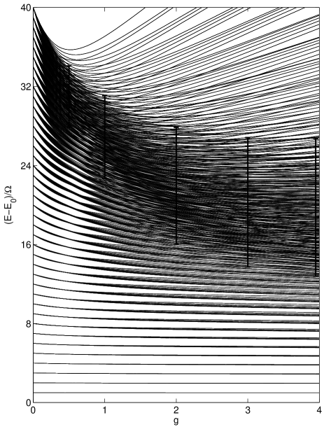
Figure 1: Low-energy spectrum of the 3-sites BH-model for $N=40$. The energy is measured with respect to the ground energy $E_{0}$ and scaled with respect to the Bogoliubov frequency $\Omega$. Error bars indicate the energy intervals, where the classical counterpart of the system shows chaotic dynamics.

As an intermediate step, let us derive the Bogoliubov spectrum (7) by using semiclassical arguments. The classical counterpart of the Hamiltonian (2) is obtained by scaling it with respect to the total number of particles, $\widehat{H}/N\rightarrow H$, and identifying the operators $\hat{b}_{k}^{\dagger}/\sqrt{N}$ and $\hat{b}_{k}/\sqrt{N}$ with pairs of canonically conjugated variables $(b^{*}_{k},b_{k})$. Next we switch to the action-angle variable, $b_{k}=\sqrt{I_{k}}\exp(i\theta_{k})$, and explicitly take into account that $\sum_{k}I_{k}=1$ is an integral of motion. This reduces our system of 3 degrees of freedom to a system of two degrees of freedom,

$$\begin{array}[]{lll}H&=&(\delta+g)(I_{-1}+I_{+1})+2gI_{0}\sqrt{I_{-1}I_{+1}}\cos(\theta_{-1}+\theta_{+1})\\ &-&g(I_{-1}I_{+1}+I_{-1}^{2}+I_{+1}^{2})\\ &+&2g\sum_{\pm}I_{\mp}\sqrt{I_{0}I_{\pm 1}}\cos(2\theta_{\mp 1}-\theta_{\pm 1})\;,\end{array}$$ (8)

where $I_{0}=1-I_{-1}-I_{+1}$ and the phases $\theta_{\pm 1}$ of variables $b_{\pm 1}(t)$ are measured with respect to the phase of $b_{0}(t)$. The low-energy dynamics of the system (8), which is associated with the low-energy spectrum of the system (1), implies $I_{\pm 1}\ll I_{0}$. Keeping in the Hamiltonian (8) only the terms linear on $I_{\pm 1}$, and using one more canonical transformation,

$$I=I_{+1}+I_{-1}\;,\quad\theta=(\theta_{+1}+\theta_{-1})/2\;,$$ (9)

$$J=(I_{+1}-I_{-1})/2\;,\quad\vartheta=\theta_{+1}-\theta_{-1}\;,$$

we obtain

$$H_{eff}=(\delta+g)I+g\sqrt{I^{2}-4J^{2}}\cos(2\theta)\;.$$ (10)

[Note that for $J=0$ this Hamiltonian coincides with the classical counterpart ($\hat{n}/N\rightarrow I$) of the effective Hamiltonian (6).] Finally, we integrate the system (10) by introducing a new action,

$$\tilde{I}=\frac{1}{2\pi}\oint I(\theta,\widetilde{E})d\theta\;,$$ (11)

and resolving Eq. (11) with respect to the energy. This gives

$$\widetilde{E}=\Omega\tilde{I}\;,\quad\Omega=\sqrt{2g\delta+\delta^{2}}\;,\quad\tilde{I}\ll 1\;.$$ (12)

Note that the energy is independent of the action $J$, which may be chosen arbitrary in the interval $|J|\leq\tilde{I}/2$. Referring to the original quantum problem, this action $J$ obviously labels the degenerate sublevels of the excited Bogoliubov states remark0 .

Now we are prepared to discuss the finite-$N$ corrections to the Bogoliubov spectrum. Let us analyze the dynamics of the classical system (8) in more detail, without assuming $I_{\pm 1}\ll I_{0}$. First we shall consider the symmetric solutions, where $b_{-1}(t)=b_{+1}(t)$. Expressing the Hamiltonian (8) in terms of the canonical variables (9) and setting there $\vartheta=0$ and $J=0$, we have

$$H_{1D}=(\delta+g)I+g(1-I)I\cos(2\theta)$$ (13)

$$-3gI^{2}/4+gI\sqrt{2(1-I)I}\cos(\theta)\;.$$

The phase portrait of the 1D system (13) is depicted in Fig. 2(a). Our particular interest in this phase portrait are the trajectories near the origin $I=0$, which can be associated with the Bogoliubov states. It is seen in the figure, that these trajectories are strongly affected by the elliptic point in the upper part of the phase space. As a consequence, the eigen-frequency of the system depends on the action $\tilde{I}$. Namely, $\widetilde{\Omega}=\widetilde{\Omega}(\tilde{I})$ vanishes for the separatrix action $\tilde{I}^{*}$, and for $\tilde{I}\ll\tilde{I}^{*}$ one has

$$\widetilde{\Omega}(\tilde{I})=\Omega-\gamma\tilde{I}\;,$$ (14)

where the nonlinearity $\gamma$ is a unique function of $g$. (For instance, for $g=0.1,1,4$ we have $\gamma/\Omega=0.1,0.6,1$, respectively.) Referring to the original quantum problem the result (14) means that the energy difference between $(m+1)$-th and $m$-th Bogoliubov levels decreases as $\gamma m/N$.

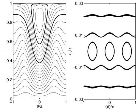
Figure 2: Left: phase portrait of the 1D system (13) for $g=1$. The bold lines restrict the chaotic region, where the trajectories are unstable with respect to variation of $(J,\vartheta)$. Right: slow dynamics of the variables $\bar{J}=\langle J\rangle$ and $\bar{\vartheta}=\langle\vartheta\rangle$ for $g=1$ and $\tilde{I}=0.133$.

Next we address the ‘stability’ of the symmetry plane trajectories depicted in Fig. 2(a) with respect to variation of $J$. Within the Bogoliubov approximation the action $J$ is an integral of motion and may be chosen arbitrary in the interval $|J|\leq\tilde{I}/2$. It should be understood, however, that in reality the action $J$ does depend on time. An example of this dependence is given in Fig. 3. It is seen that the time evolution of the system is a superposition of fast dynamics, where $J(t)$ and $\vartheta(t)$ oscillate with the Bogoliubov frequency (more precisely, with the frequency $\widetilde{\Omega}$), and slow dynamics, with the characteristic frequency of the orders of magnitude smaller than the Bogoliubov frequency. Going ahead, we note that this new frequency defines the splitting of the Bogoliubov levels in Fig. 1, and for the moment we only stress that the system dynamics remains regular. This conclusion holds for any trajectory of the effective 1D system (13), providing that the trajectory lies well below the separatrix. If we choose a trajectory closer to the separatrix, we observe a transition from regular to chaotic dynamics. We identify the exact border of the transition to chaos by calculating the Poincare cross-section of (8) for different values of the energy $\widetilde{E}$ and evaluating the volume of the chaotic component as the function of energy remark1 . It is found that the chaotic region is restricted to a relatively narrow energy interval $\widetilde{E}_{min}(g)\leq\widetilde{E}\leq\widetilde{E}_{max}(g)$. For $g=1$ the phase trajectories of the system (13), corresponding to $\widetilde{E}_{min}$ and $\widetilde{E}_{max}$, are marked by the bold lines in Fig. 2(a). Additionally, the error bars in Fig. 1 indicate the chaotic energy intervals for different values of $g$. The depicted borders are consistent with the visual analysis of the spectrum and suggest the following simple criteria of the transition to chaos: it takes place when the total splitting of the Bogoliubov levels with respect to the second quantum number exceeds the mean distance $\widetilde{\Omega}$ between the levels.

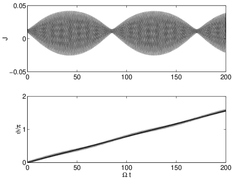
Figure 3: An example of time evolution of the conjugated variables $J(t)$ and $\vartheta(t)$ in the regular regime. Parameters correspond to the second from top trajectory in Fig. 2(a).

The question on the sublevels splitting is in turn. As it was already mentioned, this splitting is defined by the slow dynamics of the system. To address this slow dynamics we introduce the new variables $\bar{J}=(1/2\pi)\oint Jd\tilde{\theta}$ and $\bar{\vartheta}=(1/2\pi)\oint\vartheta d\tilde{\theta}$, where $\tilde{\theta}=\widetilde{\Omega}t$ is the phase conjugated to the action $\tilde{I}$. (Note that the action $\tilde{I}$ is an adiabatic integral of motion and, hence, does not depend on time.) The Hamiltonian equations of the motion for the variables $\bar{J}$ and $\bar{\vartheta}$ read,

$$\begin{array}[]{lllll}\dot{\bar{\vartheta}}&=&\langle\partial H/\partial\vartheta\rangle&\approx&-2g\bar{J}\;,\\ \dot{\bar{J}}&=&-\langle\partial H/\partial J\rangle&\approx&6gV(g,\tilde{I})\sin(3\bar{\vartheta}/2)\;,\end{array}$$ (15)

where $V(g,\tilde{I})\approx\langle(I/2)^{3/2}\cos{\theta}\rangle$ and $\langle\ldots\rangle$ means time average over one period of the fast dynamics. Thus the slow dynamics is defined by the pendulum-like Hamiltonian,

$$H_{slow}=-g\bar{J}^{2}+4gV(g,\tilde{I})\cos(3\bar{\vartheta}/2)\;.$$ (16)

It is worth of noting that, to obtain (16), we have assumed the quantity $V(g,\tilde{I})$ to be independent of $\bar{J}$, which can be justified only if $\bar{J}\ll\tilde{I}/2$. Nevertheless, the Hamiltonian (16) is found to well capture the main features of the low-energy regular dynamics for arbitrary $\bar{J}$. In particular, it correctly predicts the existence of stable points at $\vartheta=0,\pm 4\pi/3$, where the phases of $b_{\pm 1}(t)$ are locked to 0 and 120 degrees with respect to each other [see Fig. 2(b)]. The size of the stability islands around these fixed points is obviously given by the separatrix trajectory of the pendulum, i.e., is proportional to $|V(g,\tilde{I})|^{1/2}$.

It is instructive to consider the limiting case $g\rightarrow 0$. As easy to show, in this limit $V(g,\tilde{I})\rightarrow 0$ and, hence, $H_{slow}=-g\bar{J}^{2}$. Let us prove that this results corresponds to the first order quantum perturbation theory on $U$. Indeed, calculating the first order corrections to the energies of the quasimomentum Fork states $|\Psi_{m,j}\rangle=|m/2-j,N-m,m/2+j\rangle$, we have $\Delta E=(U/2L)\langle\Psi_{m,j}|\sum\hat{b}_{k_{1}}^{\dagger}\hat{b}^{\dagger}_{k_{2}}\hat{b}_{k_{3}}\hat{b}_{k_{4}}\tilde{\delta}(k_{1}+k_{2}-k_{3}-k_{4})|\Psi_{m,j}\rangle\sim-(U/L)j^{2}$, or $\Delta\widetilde{E}=-g\bar{J}^{2}$, where $\bar{J}=j/N$ and $\widetilde{E}=E/N$. Thus for small $g$ the splitting between sublevels grows linearly with $g$. This linear regime changes to a nonlinear one as soon as the second term in the Hamiltonian (16) takes a non-negligible value. This second term also causes the rearrangement of the sublevels, clearly seen in Fig. 1. Needless to say that in this case the second quantum number is defined by the action $\tilde{J}=(1/2\pi)\oint\bar{J}d\bar{\vartheta}$, which amounts to the phase volume encircled by the trajectories in Fig. 2(b).

We conclude the paper by formulating quantitative criteria for the onset of Quantum Chaos. As mentioned earlier, the transition to irregular spectrum occurs when the total splitting of the $m$-th Bogoliubov level compares with the Bogoliubov frequency. Ignoring the nonlinear corrections, one has $g(m+1)^{2}/4N\sim\Omega$, or

$$m_{cr}\approx\left(\frac{4N\sqrt{\delta^{2}+2\delta g}}{g}\right)^{1/2}\;.$$ (17)

Through the relation $E_{cr}\approx\Omega m_{cr}$ this estimate defines the critical value of energy above which the regular spectrum transforms into a chaotic one.

In conclusion, we have analyzed the Bogoliubov spectrum of the BH-model. This spectrum corresponds to low-energy excitations of the system and is usually introduced by using the Bogoliubov-de Gennes transformation. This standard method, however, is rather formal and hides the underlying classical dynamics of the BH-model. In this work we use a semiclassical method which, by definition, explicitly refers to the classical dynamics and provides in this way a deeper insight in the structure of the low-energy spectrum of the system. In the present work we restricted ourselves by considering the 3-sites BH-model, although many of the reported results hold for $L>3$ as well. An advantage of the 3-sites model is that, thanks to a relative low dimensionality of the system, its classical dynamics can be understood in every detail. In particular, the phase space of the system essentially consists of two regular and one chaotic component in between, where the low-energy regular component is shown to be associated with the Bogoliubov spectrum. We identify the full set of the integrals of motion for this low-energy regular component and, quantizing them, obtain the low-energy levels of the quantum BH-model. These levels are labelled by two quantum numbers, $m$ and $j$. The first quantum number $m$ corresponds to usual Bogoliubov ladder, where the distance between neighboring levels is approximately given by the Bogoliubov frequency $\Omega$ (i.e., $E_{m+1,j}-E_{m,j}\sim\Omega$). The second quantum number $j$ labels $(m+1)$ sublevels of the $m$-th Bogoliubov level, where the splitting between the sublevels is proportional to the interaction constant $g$ and inverse proportional to the system size $N$ (i.e., $E_{m,j+1}-E_{m,j}\sim g/N$). If we go up the energy axis, the total splitting of the Bogoliubov levels compares the distances between the levels and the energy spectrum shows a transition from a regular to irregular (chaotic) one.

The described scenario of evolution of the Bogoliubov spectrum into a regular, Bogoliubov-like spectrum and further into a chaotic spectrum also holds for the BH-model with $L>3$ sites. However, to indicate the critical energies for these transitions remains an open problem. The qualitative difference between the 3-sites and, for example, 5-sites BH-models is that the latter system has two different Bogoliubov frequencies, associated with two different single-particle excitation energies. For some values of the macroscopic interaction constant $g$, these frequencies become commensurable, which strongly affects the onset of chaos. We reserve this problem of interacting Bogoliubov spectra for future studies.

Fruitful discussions with S. Tomsovic and partial support by Deutsche Forshungsgemeinschaft (within the SPP1116 program) is gratefully acknowledged.

References

- (1) L. D. Landau, J. Phys. USSR 5, 71 (1941).
- (2) A. J. Leggett, Rev. of Mod. Phys. 73, 307 (2001).
- (3) L. Cruzeiro-Hansson et. al, Phys. Rev. B 42, 522 (1990);
- (4) A.R.Kolovsky and A.Buchleitner, Europhys. Lett. 68 (2004), 632.
- (5) M. Hiller, T. Kottos, and T. Geisel, Phys. Rev. A 73, 061604 (2006).
- (6) A. R. Kolovsky, New Journal of Physics 8, 197 (2006).
- (7) J. C. Eilbeck, P. S. Lomdahl and A. C. Scott, Physica D 16, 318 (1985).
- (8) D. Hennig et al., Phys. Rev. E 51, 2870 (1995).
- (9) K. Nemoto et al., Phys. Rev. A 63, 013604 (2000).
- (10) R. Franzosi and V. Penna, Phys. Rev. A 65, 013601 (2001); Phys. Rev. E 67, 046227 (2003); P. Buonsante, R. Franzosi, and V. Penna, Phys. Rev. Lett. 90, 050404 (2003).
- (11) Since plays the role of Planck’s constant in the considered problem, the semiclassical quanitization of (13) corresponds to , , and , .
- (12) There is some freedom in defining the border of the transition to chaos. In what follows we define it as the energy below which the chaotic component occupies less than one percent of the energy shell.