Impurity resonant state in $d$-wave superconductors: in favor of a Kondo-like response

Abstract

We investigate the impurity resonant state induced by non-magnetic impurities in $d$-wave cuprate superconductors in two different impurity models: (i) in a pure potential scattering model within the $T$-matrix approach and (ii) in a Bose-Fermi Kondo model within the large-$\mathcal{N}$ formalism. We modify the superconducting host to resemble the nanoscale electronic inhomogeneities seen in the scanning tunneling microscopy (STM) spectra (i.e., the small- and large-gap domains) and study how this influences the impurity resonance. In the pure potential scattering model the resonant state is found to be a rather robust feature appearing in all host domains. On the other hand, in the Kondo-like model the impurity resonance can appear in the small-gap regions of the host and be completely suppressed in the large-gap regions; this is in agreement with the STM experimental data for Zn-doped Bi₂Sr₂CaCu₂O_8+δ. Our results imply that the Kondo spin dynamics of the impurity moment is the origin of the impurity resonant state in $d$-wave superconductors, rather than the pure potential scattering.

I Introduction

Scanning tunneling microscopy (STM) experiments on surfaces of the high temperature cuprate superconductor Bi₂Sr₂CaCu₂O_8+δ (BSCCO) provide a powerful tool for probing strong electronic correlations in this material.hudson ; panBSCCO ; langBSCCO ; uchida Since the STM measures a local density of states (LDOS) with a high real-space resolution it is widely used for studying impurity effects in $d$-wave superconductors (SC). balatskyIMP Extensive STM studies have been performed on both magnetic Ni and non-magnetic Zn impurities in BSCCO. Particularly interesting is the Zn resonant state, i.e., a large peak in the differential conductance (i.e., in the LDOS) at small but finite energy which is mainly localized near the Zn site.yazdani ; hudson ; panBSCCO Despite the fact that there are numerous theoretical studies dealing with the resonant state induced by non-magnetic impurities in $d$-wave cuprates, no consensus on the theoretical description has been reached yet.balatskyIMP

The Zn²⁺ impurity has spin $S=0$ and it might be natural to describe it as a delta-function potential scatterer within a potential scattering (PS) model.balatsky ; hirschfeld In the PS model the resonance peak can be identified with a quasibound state whose energy can be tuned by varying the strength of the potential. However, a low-energy state appears only for large potential values, i.e., in the unitary limit. Moreover, some experimental findings cannot be easily explained within the PS model like the spatial dependence of the resonance peak which shows a global maximum on the Zn site and local maxima on the next-nearest neighbor Cu sites.notefilter

Nuclear magnetic resonance (NMR) experiments are another powerful probe of strongly correlated systems like cuprates. In a series of NMR experiments it has been established that each non-magnetic impurity (e.g., Zn²⁺ or Li⁺) induces a net local $S=1/2$ moment that is distributed on the Cu ions in its vicinity.alloulNMR ; mahajanNMR ; julienNMR ; bobroff Furthermore, the effective induced moment interacts with the elementary excitations of the bulk material giving rise to Kondo-like physics which has indeed been observed in NMR experiments.bobroff Consequently, one can treat a non-magnetic Zn impurity in the $d$-wave SC within the Kondo model and identify the low-energy impurity state in the STM spectra with the Kondo resonance.polkovnikovSTM ; vojtabullaSTM However, it is still not completely settled whether the potential scattering or the Kondo-like description is more appropriate for modeling the non-magnetic impurities in the cuprates and for explaining all experimental facts.balatskyIMP The main objective of the present study is to resolve this question. In principle, Kondo-like behavior should be suppressed by an external magnetic field which would allow to identify the origin of the observed impurity STM signal. So far, no such experiments have been performed and it has been shown that for this purpose rather high magnetic fields would be needed.zitzler

Recently the STM measurements on BSCCO have revealed the presence of nanoscale electronic inhomogeneities which show up as spatial modulation of both the gap amplitude and the LDOS.howald ; panBSCCOa ; langBSCCO ; mcelroy These electronic inhomogeneities and variations of the LDOS attracted numerous theoretical and experimental studies.nunner ; mcelroySCI ; uchida Random out-of-plane dopant atoms which change the pair interaction locallynunner and a competing order like antiferromagnetismatkinson have been proposed to be a possible origin of the LDOS modulations in the cuprates. Importantly, the STM studies on BSCCO have identified two distinct electronic domains: (i) the domains with a small-gap magnitude and with well-developed SC coherence peaks and (ii) the large-gap domains without SC coherence peaks. Remarkably, in the presence of impurities it was observed that impurity resonances are present only in the small-gap domains and no impurity resonances can be detected in the large-gap domains.langBSCCO Using this experimental fact and motivated by the question about the origin of the impurity resonance in $d$-wave cuprate SC we investigate how the resonance state is influenced by putting the impurity into different domains of the SC host in both the PS model and in the Kondo model. To get quantitative results we employ a $T$-matrix and a large-$\mathcal{N}$ approach for the PS and the Kondo model, respectively. We conclude that the Zn impurity resonance in BSCCO has predominantly a Kondo-like character.

Very recently a new possibility for the origin of the Zn resonance peak in BSCCO has been proposed.andreev Namely, in $d$-wave SC short-ranged off-diagonal ($\tau^{x}$) impurities generate low-energy Andreev states which are then associated with the impurity resonance seen in the STM spectra. If the usual $\tau^{z}$ impurity scattering is absent, the Andreev resonant state exists symmetrically around the Fermi level. However, by including a weak $\tau^{z}$ potential this symmetry is broken. This gives results which bear closer resemblance to the STM data. Below, we will comment on some of these results.

The remainder of the paper is organized as follows. In Sec. II we introduce the relevant models for describing a non-magnetic impurity embedded in a $d$-wave superconductor. In Sec. III the $T$-matrix approach and the large-$\mathcal{N}$ formalism are explained. Our numerical results and a comparison with experimental data are presented in Sec. IV. We conclude the paper in Sec. V.

II The Model

To describe a single impurity atom in a superconducting material we will consider a Hamiltonian consisting of a bulk and an impurity part, $H=H_{\text{bulk}}+H_{\text{imp}}$. Both terms are specified below.

II.1 The Superconducting Host

As a model for the cuprate superconductor we use the usual BCS Hamiltonian

$$H_{\text{BCS}}^{\phantom{\dagger}}=\sum_{{\bf k}}\Psi_{\bf k}^{\dagger}\bigl{[}(\varepsilon_{\bf k}^{\phantom{\dagger}}-\mu)\tau^{z}+\Delta_{\bf k}^{\phantom{\dagger}}\tau^{x}\bigr{]}\Psi_{\bf k}^{\phantom{\dagger}},$$ (1)

where $\Psi_{\bf k}^{\dagger}=(c_{{\bf k}\uparrow}^{\dagger}\,\,\,c_{{-\bf k}\downarrow}^{\phantom{\dagger}})$ is a Nambu spinor with momentum ${\bf k}=(k_{x},k_{y})$, $c_{{\bf k}\sigma}^{\dagger}$ ($c_{{\bf k}\sigma}^{\phantom{\dagger}}$) creates (annihilates) an electron with momentum ${\bf k}$ and spin $\sigma$, and the three Pauli matrices in particle-hole space are denoted by $\tau^{x,y,z}$. We use a tight-binding dispersion of the form

$$\varepsilon_{\bf k}^{\phantom{\dagger}}=\frac{t_{1}}{2}\bigl{(}\cos k_{x}+\cos k_{y}\bigr{)}+t_{2}\cos k_{x}\cos k_{y}+\frac{t_{3}}{2}\bigl{(}\cos 2k_{x}+$$

$$\quad\quad+\cos 2k_{y}\bigr{)}+\frac{t_{4}}{2}\bigl{(}\cos 2k_{x}\cos k_{y}+\cos k_{x}\cos 2k_{y}\bigr{)}+$$

$$\quad\quad+t_{5}\cos 2k_{x}\cos 2k_{y},$$ (2)

with values for the hopping elements that fit the ARPES data:normanBSCCO $t_{1}=-0.5951$ eV, $t_{2}=0.1636$ eV, $t_{3}=-0.0519$ eV, $t_{4}=-0.1117$ eV, $t_{5}=0.0510$ eV, and $\mu=-0.1305$ eV for optimal doping ($p=19.5\,\%$). The $d$-wave pairing function is given by $\Delta_{\bf k}=\Delta_{0}\bigl{(}\cos k_{x}-\cos k_{y}\bigr{)}/2$ where $\Delta_{0}=40$ meV. In order to model the nanoscale electronic inhomogeneities seen by the STM (i.e., the small- and large-gap domains) it is necessary to modify the pure BCS state; this will be discussed in Sec. IV.1.

II.2 The Impurity Hamiltonian

We consider an effective impurity Hamiltonian which consists of a potential scattering and a magnetic term, $H_{\text{imp}}=H_{\text{pot}}+H_{\text{K}}$. The potential scattering term describes electrostatic interactions between the impurity atom and the conduction electrons whereas the magnetic term represents an impurity moment embedded in the SC host.

II.2.1 Potential Scattering Model

We assume that the potential scattering is completely localized at the impurity site ${\bf r}_{0}=(0,0)$, i.e., $V({\bf r})=V_{0}\,\delta({\bf r}-{\bf r}_{0})$. Consequently, the scattering occurs only in the isotropic $s$-wave channel and the scattering term is given by $H_{\text{pot}}^{\phantom{\dagger}}=V_{0}^{\phantom{\dagger}}\sum_{\sigma}c_{0\sigma}^{\dagger}c_{0\sigma}^{\phantom{\dagger}}$, where $c_{0\sigma}^{\phantom{\dagger}}=N^{-1/2}\sum_{\bf k}c_{{\bf k}\sigma}$, and $N$ is the number of sites. In the PS model the bulk Hamiltonian is defined as $H_{\text{bulk}}=H_{\text{BCS}}$.

II.2.2 Bose-Fermi Kondo Model

To specify the magnetic term in the impurity Hamiltonian we use the so-called Bose-Fermi Kondo model.bfkSi ; BFK1 ; BFK2 ; mvIMP It describes a spin-$1/2$ impurity, ${\bf S}_{\text{imp}}$, coupled both to the electrons of the conduction band and to a bosonic bath representing bosonic collective excitations in the host material. (Apart from its application to the impurity moments in the cuprates,BFK1 the Bose-Fermi Kondo model has attracted considerable interest in the context of local quantum criticality within an extended dynamical mean-field theory,edmft and also in certain mesoscopic systems like a quantum dot coupled to ferromagnetic leads.set )

In the $d$-wave cuprate SC it is reasonable to separate the low-energy degrees of freedom into fermionic Bogoliubov quasiparticles around the nodal points, and into bosonic antiferromagnetic spin-1 collective fluctuations near the ordering wave-vector ${\bf Q}=(\pi,\pi)$.bkVBS ; BFK1 ; BFK2 The effective impurity moment induced by non-magnetic impurity interacts with both the fermionic and the bosonic bulk excitations. Therefore, a non-magnetic impurity in cuprates is expected to be well described by the Bose-Fermi Kondo modelBFK1

$$H_{\text{K}}^{\phantom{\dagger}}=J_{\text{K}}^{\phantom{\dagger}}\,{\bf S}_{\text{imp}}^{\phantom{\dagger}}\cdot{\bf s}_{0}^{\phantom{\dagger}}+\gamma_{0}^{\phantom{\dagger}}\,{\bf S}_{\text{imp}}^{\phantom{\dagger}}\cdot{\boldsymbol{\phi}}_{0}^{\phantom{\dagger}}.$$ (3)

Here, ${\bf s}_{0}^{\phantom{\dagger}}=1/(2N)\sum_{{\bf kk^{\prime}}\sigma\sigma^{\prime}}c_{{\bf k}\sigma}^{\dagger}{\boldsymbol{\sigma}}_{\sigma\sigma^{\prime}}^{\phantom{\dagger}}c_{{\bf k^{\prime}}\sigma^{\prime}}^{\phantom{\dagger}}$ is the conduction electron spin operator at the impurity site, ${\boldsymbol{\sigma}}$ are the Pauli matrices in spin space, and $J_{\text{K}}$ is the usual Kondo coupling. The impurity moment is coupled to the bosonic bath via a coupling constant $\gamma_{0}$. The local field ${\boldsymbol{\phi}}_{0}$ represents the local orientation of the antiferromagnetic order parameter and it is given by ${\phi}_{0\gamma}^{\phantom{\dagger}}=\sum_{\bf q}(b^{\phantom{\dagger}}_{{\bf q}\gamma}+b^{\dagger}_{-{\bf q}\gamma})\sqrt{2JA_{\bf q}/\omega_{\bf q}}$, where $J$ is the bulk exchange constant, $A_{\bf q}$ is a dimensionless function containing the geometry of the system, and $\gamma=x,y,z$.bkVBS The simplest bosonic bath consists of free vector bosons, $H_{\text{bos}}^{\phantom{\dagger}}=\sum_{{\bf q}\gamma}\omega_{\bf q}^{\phantom{\dagger}}b_{{\bf q}\gamma}^{\dagger}b_{{\bf q}\gamma}^{\phantom{\dagger}}$, with the dispersion $\omega_{\bf q}^{2}=m^{2}+c^{2}{\bf q}^{2}$, where the momentum ${\bf q}$ is measured relative to the ordering wave-vector ${\bf Q}$ and $c$ is the velocity of the spin excitations.bkVBS At zero temperature, the effective bosonic mass $m$ is equivalent to the bulk spin gap $\Delta_{\text{s}}$ (as seen in neutron scattering experimentsfong ). A spin gap $\Delta_{\text{s}}=0$ corresponds to a bulk quantum-critical point controlling a transition between a quantum paramagnet ($\Delta_{\text{s}}>0$) and the antiferromagnetically ordered phase.bkVBS

In the present study the Kondo Hamiltonian (3) describes the physics of the so-called pseudogap (i.e., softgap) Bose-Fermi Kondo model.BFK1 ; BFK2 There, a fermionic LDOS follows a power-law close to the Fermi energy, $\rho_{c}^{0}(\omega)\sim|\omega|^{r}$, where $\omega$ is measured from the Fermi level. Clearly, the $d$-wave superconductor has $r=1$. In addition, at zero temperature and for $\Delta_{\text{s}}=0$, the bosonic LDOS also follows a power-law, $\rho_{\phi}^{0}\sim\text{sgn}(\omega)|\omega|^{1-\epsilon}$, where $\epsilon=3-d$, and $d$ is the dimension of the system (for cuprates $d=2$). It is important to note that for $\gamma_{0}=0$ the Bose-Fermi Kondo model (3) reduces to the extensively studied fermionic pseudogap Kondo model.withofffradkin ; cassanellofradkin ; ingersent ; vojtabullaSTM Depending on the value of $r$ and the presence or absence of particle-hole symmetry, the fermionic pseudogap Kondo model exhibits a quantum phase transition between a phase with Kondo screening for $J_{\text{K}}>J_{\text{Kc}}$, and a phase where the magnetic moment is free (i.e., decoupled from the bath) for $J_{\text{K}}<J_{\text{Kc}}$. It is also known that the presence of an additional bosonic bath for $\gamma_{0}\neq 0$, leads to a suppression of the Kondo screening.bfkSi ; BFK1 ; BFK2 Note that in the present analysis we will use the Bose-Fermi Kondo model with the bulk Hamiltonian $H_{\text{bulk}}=H_{\text{BCS}}+H_{\text{bos}}$.notecoupling

To describe non-magnetic impurities like Zn (or Li) in the copper oxide planes it is appropriate to use the so-called extended magnetic impurity.polkovnikovSTM ; vojtabullaSTM NMR experiments have shown that the effective moment induced by a non-magnetic impurity is spatially distributed around the impurity site, ${\bf r}_{0}$, and mainly resides on the four nearest neighbor copper sites.julienNMR Therefore, the Kondo model with an extended magnetic impurity is required in order to explain both the STM and NMR measurements on cuprates with non-magnetic impurities.polkovnikovSTM ; vojtabullaSTM In the present calculation we consider a four-site Kondo model in $d$-wave superconductors where the effective magnetic moment is coupled to the four Cu sites ${\bf s}=(\pm 1,0),(0,\pm 1)$ adjacent to the impurity. One should bare in mind that in this four-site model the effective LDOS of the fermionic bath seen by the impurity changes; this will be shortly discussed in Sec. III.2.1.

III Method

We start with the definition of the conduction electron Green’s function in the absence of impurities, which is given by $\underline{\mathcal{G}}_{\,c}^{0}(\tau,{\bf k})=-\langle T_{\tau}^{\phantom{\dagger}}\Psi_{\bf k}^{\phantom{\dagger}}(\tau)\Psi_{\bf k}^{\dagger}(0)\rangle$. (In our notation all underlined symbols denote matrices.) Its Fourier transform is given by $\underline{\mathcal{G}}_{\,c}^{0}(i\nu_{n},{\bf k})=\int_{0}^{\beta}\text{d}\tau\,\underline{\mathcal{G}}_{\,c}^{0}(\tau,{\bf k})\,\text{e}^{i\nu_{n}\tau}$, where $\nu_{n}=(2n+1)\pi T$ represents the fermionic Matsubara frequencies and $\beta$ is the inverse temperature. Note that the bare Green’s function in real space is simply given by $\underline{\mathcal{G}}_{\,c}^{0}(i\nu_{n},{\bf r})=N^{-1}\sum_{\bf k}\text{e}^{i{\bf k}\cdot{\bf r}}[i\nu_{n}-(\varepsilon_{\bf k}-\mu)\tau^{z}-\Delta_{\bf k}\tau^{x}]^{-1}$.

III.1 $T$-matrix Approach

The single scatterer problem, $H_{\text{pot}}$, can be solved exactly with the usual result for the perturbed Green’s functionbalatskyIMP

$$\underline{\mathcal{G}}_{\,c}(i\nu_{n},{\bf r},{\bf r^{\prime}})=\underline{\mathcal{G}}_{\,c}^{0}(i\nu_{n},{\bf r}-{\bf r^{\prime}})+$$

$$\hskip 28.45274pt+\underline{\mathcal{G}}_{\,c}^{0}(i\nu_{n},{\bf r}-{\bf r}_{0})\,\underline{T}(i\nu_{n})\,\underline{\mathcal{G}}_{\,c}^{0}(i\nu_{n},{\bf r}_{0}-{\bf r^{\prime}}),$$ (4)

where the $T$-matrix is given by

$$\underline{T}(i\nu_{n})=V_{0}\,\tau^{z}\bigl{[}\underline{1}-V_{0}\,\underline{\mathcal{G}}_{\,c}^{0}(i\nu_{n},{\bf r}_{0})\,\tau^{z}\bigr{]}^{-1}.$$ (5)

The $T$-matrix depends on the strength of the scattering potential and on the local conduction electron Green’s function, $\underline{\mathcal{G}}_{\,c}^{0}(i\nu_{n},{\bf r}_{0})$. It is important to note that this local Green’s function is the only input quantity representing the bulk material; it differs significantly in the small-gap and the large-gap regions of the SC host (more details are given in Sec. IV.1).

III.2 Large-$\mathcal{N}$ Formalism

In order to obtain quantitative results in the Bose-Fermi Kondo model we use the large-$\mathcal{N}$ formalism. The large-$\mathcal{N}$ theory can be constructed by generalizing the spin symmetry of the impurity moment, the conduction electrons, and the vector bosons from SU(2) to SU($\mathcal{N}$). An antisymmetric representation of the impurity spin is given by ${\bf S}_{\text{imp}}^{\mu\mu^{\prime}}=f_{\mu}^{\dagger}f_{\mu^{\prime}}^{\phantom{\dagger}}-q_{0}^{\phantom{\dagger}}\delta_{\mu\mu^{\prime}}^{\phantom{\dagger}}$ with the constraint $\sum_{\mu}f_{\mu}^{\dagger}f_{\mu}^{\phantom{\dagger}}=q_{0}^{\phantom{\dagger}}\mathcal{N}$, where $f_{\mu}^{\dagger}$ ($f_{\mu}^{\phantom{\dagger}}$) creates (annihilates) auxiliary fermions with $\mu=1,\ldots,\mathcal{N}$ spin flavors. The constraint is enforced by introducing a Lagrange multiplier $\lambda_{0}$. The generalization of the spin symmetry leads to $\mathcal{N}^{2}-1$ triplet bosons denoted by $b_{{\bf q}\mu\mu^{\prime}}$.bkVBS In what follows we consider only the particle-hole symmetric case for which $q_{0}=1/2$. Therefore, in the large-$\mathcal{N}$ formalism the impurity Hamiltonian (3) is given by

$$H_{\text{K}}=\frac{J_{\text{K}}}{\mathcal{N}}\sum_{\mu\mu^{\prime}}f_{\mu}^{\dagger}f_{\mu^{\prime}}^{\phantom{\dagger}}c_{0\mu}^{\dagger}c_{0\mu^{\prime}}^{\phantom{\dagger}}+\frac{\gamma_{0}}{\sqrt{\mathcal{N}}}\sum_{\mu\mu^{\prime}}f_{\mu}^{\dagger}f_{\mu^{\prime}}^{\phantom{\dagger}}\phi_{0\mu\mu^{\prime}}^{\phantom{\dagger}}+$$

$$\quad\quad+\lambda_{0}\Bigl{(}\sum_{\mu}f_{\mu}^{\dagger}f_{\mu}^{\phantom{\dagger}}-q_{0}^{\phantom{\dagger}}\mathcal{N}\Bigr{)}.$$ (6)

It is important to emphasize that in the limit $\mathcal{N}\to\infty$ physics of both the fermionic Kondo model and the Bose Kondo model is controlled by a corresponding saddle point.readnewns ; bkVBS

We proceed with defining the pseudo-fermion Green’s function $\mathcal{G}_{f}^{0}(\tau)=-\langle T_{\tau}f(\tau)f^{\dagger}(0)\rangle$ and its Fourier transform $\mathcal{G}_{f}^{0}(i\nu_{n})=(i\nu_{n}-\lambda_{0})^{-1}$. We drop the spin indices since the SU($\mathcal{N}$) symmetry is preserved. The full pseudo-fermion Green’s function is determined from the Dyson equation

$$\mathcal{G}_{f}^{-1}(i\nu_{n})=\bigl{[}\mathcal{G}_{f}^{0}(i\nu_{n})\bigr{]}^{-1}-\Sigma_{f}(i\nu_{n}),$$ (7)

where the self-energy $\Sigma_{f}(i\nu_{n})$ has to be calculated. In addition, the Lagrange multiplier, $\lambda_{0}$, can be determined by employing the occupation constraint for the pseudo-fermions, which yields

$$\frac{1}{2}\equiv q_{0}=\langle f^{\dagger}f\rangle,\hskip 14.22636pt\text{where}\hskip 14.22636pt\langle f^{\dagger}f\rangle=\mathcal{G}_{f}(\tau=0^{-}).$$ (8)

In order to determine $\Sigma_{f}(i\nu_{n})$ in the Bose-Fermi Kondo model we first briefly present the known results for two limiting cases, namely for (i) the fermionic Kondo, $\gamma_{0}=0$, and (ii) the Bose Kondo model, $J_{\text{K}}=0$.

III.2.1 Fermionic Kondo Model: $\gamma_{0}=0$

For $\gamma_{0}=0$ by using a simple decoupling approximation one can obtain the non-interacting form of the Kondo Hamiltonian (III.2), i.e., $H_{\text{K}}^{\phantom{\dagger}}=\sum_{\mu}\bigl{[}-(vf_{\mu}^{\dagger}c_{0\mu}^{\phantom{\dagger}}+\text{h.c.})+\lambda_{0}f_{\mu}^{\dagger}f_{\mu}^{\phantom{\dagger}}\bigr{]}$ with the self-consistently determined condensation amplitude $v=J_{\text{K}}^{\phantom{\dagger}}/\mathcal{N}\sum_{\mu}\langle c_{0\mu}^{\dagger}f_{\mu}^{\phantom{\dagger}}\rangle$. This scheme, the so-called slave-boson mean-field approximation, becomes exact in the limit $\mathcal{N}\to\infty$ when the physics is dominated by a static saddle point. The known result for the pseudo-fermion self-energy is given bymvIMP

$$\Sigma_{f}^{(\text{f})}(i\nu_{n})=v^{2}\,\mathcal{G}_{c}^{0}(i\nu_{n},{\bf r}_{0}),$$ (9)

where $\mathcal{G}_{c}^{0}(i\nu_{n},{\bf r}_{0})=\text{Tr}\bigl{[}\underline{\mathcal{G}}_{\,c}^{0}(i\nu_{n},{\bf r}_{0})(\underline{1}+\tau^{z})/2\bigr{]}$ is the local Green’s function of the fermionic bath; for $V_{0}\neq 0$ one should use (III.1) instead. The condensation amplitude, $v$, measures the interaction between the conduction electrons and the impurity spin. The non-zero value of $v$ signals Kondo screening whereas for $v=0$ the moment is unscreened (free). $v$ can be determined by calculating the corresponding expectation value of the bosonic operator $c^{\dagger}_{0}f$ which is related to the mixed propagator $\mathcal{G}_{fc}(\tau)=-\langle T_{\tau}f(\tau)c_{0}^{\dagger}(0)\rangle$. Hence,

$$v=J_{\text{K}}^{\phantom{\dagger}}\langle c^{\dagger}_{0}f\rangle,\hskip 14.22636pt\text{where}\hskip 14.22636pt\langle c^{\dagger}_{0}f\rangle=\mathcal{G}_{fc}(\tau=0^{-}).$$ (10)

A simple diagrammatic analysis leads to

$$\mathcal{G}_{fc}(i\nu_{n})=-v\,\mathcal{G}_{f}(i\nu_{n})\,\mathcal{G}_{c}^{0}(i\nu_{n},{\bf r}_{0}).$$ (11)

The factor $v$ arises due to the fact that no bare mixed propagator exists and the minus sign as a result of the anticommutation relations. A non-zero condensation amplitude, $v$, at $T=0$, decreases with increasing temperature and vanishes continuously at the so-called Kondo temperature, $T_{\text{K}}$.

The equations (7)-(11) are a self-consistent system of equations for determining the full $f$-propagator, the condensation amplitude, $v$, and the Lagrange multiplier, $\lambda_{0}$. These equations can be solved for a given Kondo coupling, $J_{\text{K}}$, and a local conduction Green’s function at the impurity site. From the full $f$-propagator we can easily obtain the pseudo-fermion spectral function, $\rho_{f}(\omega)=-\text{Im}\,\mathcal{G}_{f}(\omega+i0^{+})/\pi$. A trivial solution of the self-consistent system of equations is given by $v=0$ and $\lambda_{0}=0$, which corresponds to an impurity spin which is completely decoupled from the conduction electrons. At high enough temperature this is the only solution. With decreasing temperature another non-trivial solution with $v\neq 0$ can appear. The non-trivial solution signaling the Kondo screening arises only below the Kondo temperature and for $J_{\text{K}}>J_{\text{Kc}}$. Note that $T_{\text{K}}$ can be determined for a given $J_{\text{K}}$ using (10) in the limit $v\to 0$, $\lambda_{0}\to 0$; at zero temperature we use (10) in the same limit to calculate the critical value of the Kondo coupling, $J_{\text{Kc}}$.

It is known that the slave-boson mean-field method has numerous artifacts at finite temperatures or in the vicinity of the quantum critical point for $\mathcal{N}=2$ which is the case of physical interest. Nevertheless, this approach has been extensively used in the context of the pseudogap Kondo modelwithofffradkin ; cassanellofradkin ; polkovnikov and is known to capture the qualitative physics of the Kondo screened phase.

We emphasize that in the four-site Kondo model, which we use in the present study, the LDOS seen by the impurity is given by the effective propagator $\sum_{{\bf s},{\bf s^{\prime}}}\varphi_{\bf s}\varphi_{\bf s^{\prime}}\text{Tr}\bigl{[}\underline{\mathcal{G}}_{\,c}(i\nu_{n},{\bf s},{\bf s^{\prime}})(\underline{1}+\tau^{z})/2\bigr{]}$. The Green’s function $\underline{\mathcal{G}}_{\,c}$ is defined in Eq. (III.1) (i.e., if the potential scattering is present, $V_{0}\neq 0$, we assume that it is located at the impurity site, ${\bf r}_{0}$) and $\varphi_{\bf s}=+[-]1$ for ${\bf s}-{\bf r}_{0}=(\pm 1,0)[(0,\pm 1)]$. For a more detailed discussion see Ref. vojtabullaSTM, .

III.2.2 Bose Kondo Model: $J_{\text{K}}=0$

For $J_{\text{K}}=0$ the Bose-Fermi Kondo model reduces to the so-called Bose Kondo model. In the large-$\mathcal{N}$ limit the pseudo-fermion self-energy is given bybkVBS

$$\Sigma_{f}^{(\text{b})}(i\nu_{n})=-\frac{\gamma_{0}^{2}}{\beta}\sum_{i\omega_{n}}\mathcal{G}_{f}(i\nu_{n}+i\omega_{n})\,\mathcal{D}_{\phi}^{0}(i\omega_{n},{\bf r}_{0}),$$ (12)

where $\mathcal{D}^{0}_{\phi}(\tau,{\bf r}_{0})=-\langle T_{\tau}^{\phantom{\dagger}}\phi_{0}^{\phantom{\dagger}}(\tau)\phi_{0}^{\dagger}(0)\rangle$ is the local Green’s function of the bosonic bath. The self-energy $\Sigma_{f}^{(\text{b})}(i\nu_{n})$ is derived by summing all diagrams with non-crossing bosonic lines (the so-called “rainbow” diagrams) which is known as the non-crossing approximation (NCA).bkVBS ; mvIMP The self-consistency is obtained using (7), (8), and (12).

Interestingly, in the Bose Kondo model there is always a non-trivial interaction between the impurity and the bosonic bath, i.e., $\Sigma_{f}^{(\text{b})}(i\nu_{n})\neq 0$. At zero temperature and at the bulk quantum critical point ($m=\Delta_{\text{s}}=0$ and $\omega_{\bf q}=cq$) the self-consistent solution yields a power-law behavior for the pseudo-fermion spectral function, $\rho_{f}(\omega)\sim|\omega|^{\epsilon/2-1}$. This behavior does not correspond to the usual Kondo screening which occurs in the fermionic Kondo model, but rather reflects non-trivial fluctuations that are usually referred to as the bosonic fractional (fluctuating) phase. For finite but small $\Delta_{\text{s}}$ there are no bulk spin excitations at low energies. For $\omega\ll\Delta_{\text{s}}$ the impurity moment is decoupled from the bath while the case $\omega\gg\Delta_{\text{s}}$ is analogous to the case $\Delta_{\text{s}}=0$; the crossover between these two regimes has been studied in detail in Ref. bkVBS, .

III.2.3 Bose-Fermi Kondo Model

A generalization of the large-$\mathcal{N}$ approach for the Bose-Fermi Kondo model cannot be done in a straightforward manner and further approximations are necessary. (We note, however, that the large-$\mathcal{N}$ analysis has been applied to a multi-channel version of the Bose-Fermi Kondo model.bfkLN ) Guided by the fact that the physics of both the fermionic and the bosonic Kondo model is controlled by a saddle point in the $\mathcal{N}\to\infty$ limit, we combine both effects through the pseudo-fermion self-energy

$$\Sigma_{f}^{\phantom{\dagger}}(i\nu_{n})=\Sigma_{f}^{(\text{f})}(i\nu_{n})+\Sigma_{f}^{(\text{b})}(i\nu_{n}).$$ (13)

The fermionic part obtained within the slave-boson mean-field approach (9) and the bosonic NCA contribution (12) are only formally decoupled. Their mutual effect can be easily understood through the self-consistency which we present below. Namely, diagrams containing both the conduction electron and the bosonic propagators are included through the full $f$-propagator in $\Sigma_{f}^{(\text{b})}(i\nu_{n})$. In addition, according to Eq. (11) the mixed propagator, $\mathcal{G}_{fc}$, also contains the full pseudo-fermion propagator. Therefore, the interaction with the bosonic bath entering the mixed propagator through $\mathcal{G}_{f}$ influences the condensation amplitude, i.e., Kondo screening.

The system of equations (7)-(13) can be solved self-consistently in order to obtain the full $f$-propagator, $v$, and $\lambda_{0}$ for given couplings $J_{\text{K}}$ and $\gamma_{0}$, and for given local Green’s functions of the fermionic and the bosonic bath, $\mathcal{G}_{c}^{0}(i\nu_{n},{\bf r}_{0})$ and $\mathcal{D}_{\phi}^{0}(i\omega_{n},{\bf r}_{0})$, respectively; the results obtained by numerically solving this self-consistent system are presented Sec. IV.3.

Before we show our numerical results in the next section, we discuss some limiting cases. For small coupling $J_{\text{K}}$ and the fermionic bath exponent $r>0$ we expect no Kondo screening, $v=0$, and that the problem reduces to the Bose Kondo model. On the other hand, for large $J_{\text{K}}$ and small $\gamma_{0}$ the pseudo-fermion self-energy is dominated by its fermionic term and we should recover the results of the fermionic pseudogap Kondo model. Consequently, the two interactions of the impurity with the fermionic and the bosonic bath (i.e., the fermionic and the bosonic Kondo physics) compete; the same conclusion has been reached within the renormalization group approach.bfkSi ; BFK1 ; BFK2

For $m=\Delta_{\text{s}}=0$ there is a quantum phase transition between a fermionic Kondo-dominated phase, for $J_{\text{K}}\gg\gamma_{0}$, and a bosonic fluctuation-dominated phase, for $J_{\text{K}}\ll\gamma_{0}$. Note that there is no zero temperature free moment phase as long as $\gamma_{0}\neq 0$ and $m=\Delta_{\text{s}}=0$; this is the so-called bosonic fractional moment phase.bkVBS An interesting quantity is $T_{\text{K}}=T_{\text{K}}(J_{\text{K}})$ where the Kondo screening sets in. It can be derived using Eq. (10) provided that $v\to 0$ and $\lambda_{0}\to 0$. In our calculation we determine the critical value of the Kondo coupling, $J_{\text{Kc}}$, in the $T_{\text{K}}\to 0$ limit.

IV Results

In this section we present our numerical results which are obtained for a system at zero temperature. First we explain the way in which the LDOS of the host SC is modified. Afterwards, we show the results for both (i) the pure PS model and (ii) the Kondo model with and without the potential scattering at the impurity site. Finally, we compare them with the existing STM experimental data.

IV.1 Host Local Density of States

As already noted recent STM measurements of the LDOS in cuprates have led to numerous studies; they deal with the possible origin of the nanoscale spatial variationmcelroySCI ; nunner ; uchida or identify the processes contributing to the tunneling spectra.pilgram In the present calculation we do not attempt to explain the origin of the nanoscale inhomogeneities but we model the host LDOS in a way to get close resemblance to the STM data.langBSCCO ; mcelroy

The STM experiments have established that the LDOS shows a nanoscale spatial modulation with two types of regions:howald ; langBSCCO (i) The first type corresponds to domains with small gaps and well-defined coherence peaks. In this region we assume that the BCS Hamiltonian (1) describes the bulk superconductor and we use the conduction electron Green’s function defined in Eq. (III.1) to obtain the LDOS. (ii) The second type of domains have large gaps and very broad gap-edge peaks whose amplitude is relatively low. In the following we will refer to these regions as the “pseudogaps”.

In order to describe the host superconductor in the “pseudogap” domains we use a rather phenomenological approach. We write the conduction electron Green’s function as $[\underline{\tilde{\mathcal{G}}}_{\,c}(i\nu_{n},{\bf k})]^{-1}=[\underline{\mathcal{G}}_{\,c}^{0}(i\nu_{n},{\bf k})]^{-1}-\underline{\Sigma}_{\,c}(i\nu_{n},{\bf k})$, where the bare propagator is the propagator in the pure BCS state. The main approximation enters through the form of the conduction electron self-energy, $\underline{\Sigma}_{\,c}(i\nu_{n},{\bf k})$, which we do not calculate but we employ a simple model for it. (For a thorough discussion about the conduction electron self-energy we refer the reader to Ref. chubukov1, .) It is important to note that the self-energy is chosen in such a way that the corresponding LDOS obtained from the perturbed Green’s function, $\underline{\tilde{\mathcal{G}}}_{\,c}(i\nu_{n},{\bf k})$, mimics the LDOS measured by the STM on BSCCO.langBSCCO ; mcelroy ; mcelroySCI As already mentioned, the local Green’s function of the host SC is used further as an input (i.e., a given) quantity for the $T$-matrix and the large-$\mathcal{N}$ calculations. We assume that the imaginary part of the self-energy is given by $\Sigma_{11}^{\prime\prime}(\omega,{\bf k})\sim-\omega^{2}/\Delta_{0}$ for $|\omega|\leq\Delta_{0}$, and $\Sigma_{11}^{\prime\prime}(\omega,{\bf k})\sim-\Delta_{0}$ otherwise.note_k The $\omega^{2}$-dependence ensures that the low-energy region of the LDOS (e.g., for $\omega\ll\Delta_{0}$) is not modified in all nanoscale domains which is in accordance with the STM measurements.langBSCCO ; mcelroy The real part of the self-energy is obtained by using the Kramers-Kronig relation. In addition, for simplicity we assume that $\Sigma_{11}=\Sigma_{12}=\Sigma_{21}^{\ast}=\Sigma_{22}$.

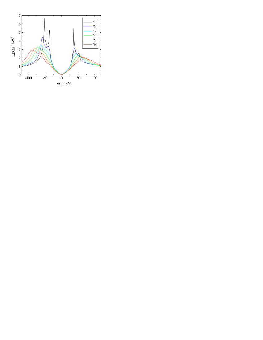
Figure 1: (color online) The different local densities of states (LDOS) of the bulk superconductor which are used as inputs for the $T$-matrix and the large-$\mathcal{N}$ calculations. By going from a pure BCS state (denoted by “1”) towards a “pseudogap” state (denoted by “6”) the gap value increases and the superconducting coherence peaks disappear. The low-energy region remains unchanged.

The host LDOS which we use in the present calculation are shown in Fig. 1 and are denoted by $``1,\ldots,6"$. The case “1” corresponds to the pure BCS state with well-defined coherence peaks and a small gap while in other spectra the gap increases and the coherence peaks disappear. In this way we can model the STM spectra with small (large) gap regions with (without) SC coherence peaks. Furthermore, the STM measurements show that the low-energy region close to the Fermi level remains unchanged;langBSCCO ; mcelroy this feature is also captured in Fig. 1. Note that larger gap values correspond to a lower hole doping level; we use the gap values $(1.0,\,1.1,\,1.2,\,1.4,\,1.6,\,1.8)\,\Delta_{0}$ for the spectra $``1,\ldots,6"$, respectively. By adjusting the chemical potential $\mu$ one obtains the correct doping; more precisely we fixed $\mu=-$($130.5$,$\,125$,$\,120$,$\,115$,$\,110$,$\,105$) meV for the doping levels $p=$($19.5$,$\,17.5$,$\,15.9$,$\,14.5$,$\,13.1$,$\,11.8$)$\,\%$.note_gap It is important to emphasize that the doping level does not significantly change our results and it can be in principle completely ignored. Nevertheless, we include the different dopings in order to model the experimental situation as close as possible.

IV.2 Potential Scattering

We start our discussion with the pure PS model ($J_{\text{K}}=\gamma_{0}=0$). It is known that the delta-function potential scatterer generates a resonant state in the superconductor LDOS and the resonance can be tuned towards the Fermi level by increasing $V_{0}$; the low-energy resonant state is possible only in unitary limit, i.e., when $V_{0}$ is the largest energy scale in the problem. However, the PS model is not able to explain the spatial distribution of the resonance which is seen in STM experiments.panBSCCO ; notefilter These results are summarized, for instance, in Fig. 1 of Ref. andreev, .

Here, we consider a non-magnetic impurity as a pure potential scatterer placed in different regions of the $d$-wave superconductor; those regions are characterized by the corresponding host LDOS (shown in Fig. 1). In Fig. 2 we show the LDOS in a $d$-wave SC at the impurity site obtained within the $T$-matrix approach for a given $V_{0}$ and different host LDOS. The potential scattering strength is chosen such that one gets a resonance in the low-energy region.

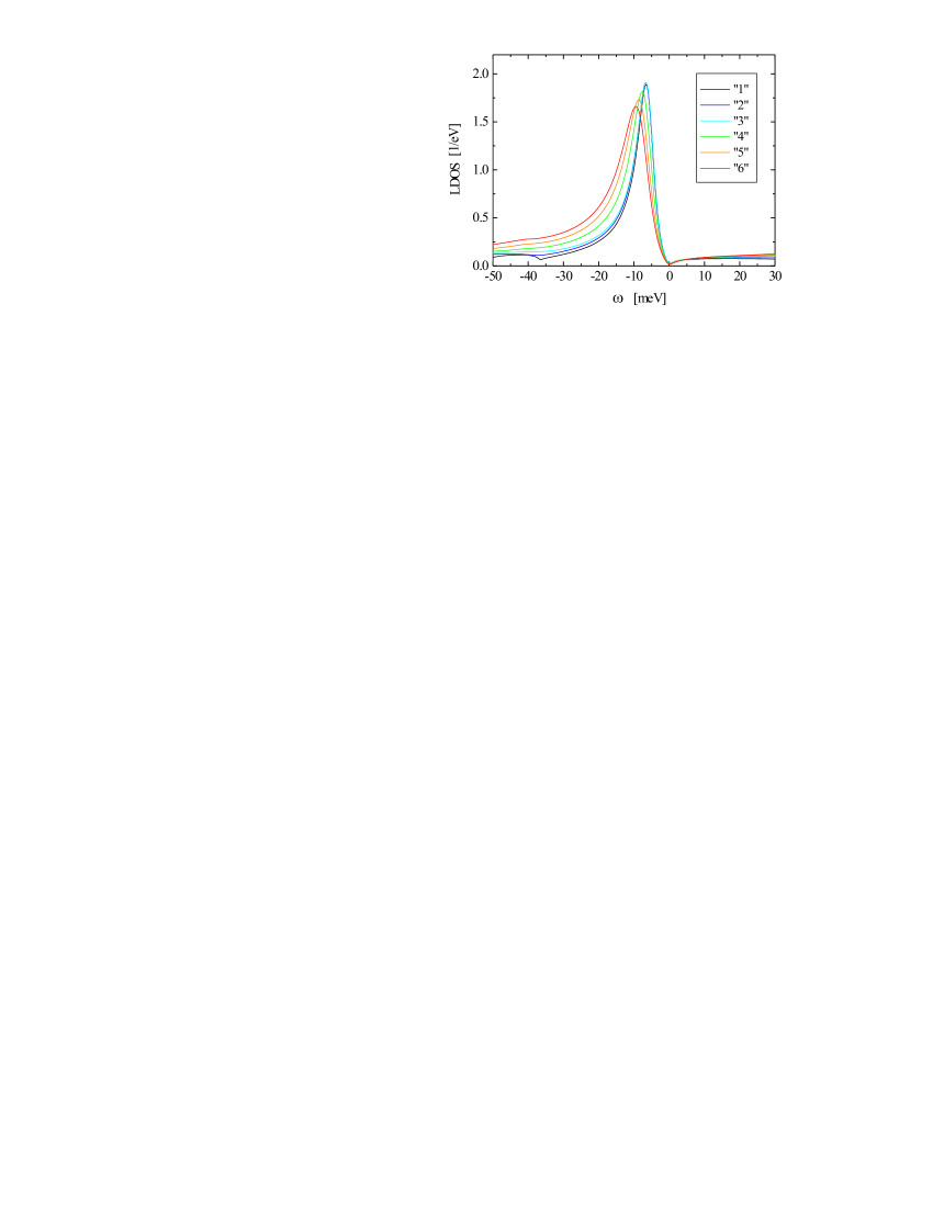
Figure 2: (color online) LDOS at the impurity site in the PS model for $V_{0}=0.2$ eV and different host LDOS. A resonance appears at a low-energy scale $\sim\mathcal{O}(\text{meV})$; it is slightly suppressed and moved away from the Fermi level by modifying the superconducting host, i.e., by going from “1” to “6” in Fig. 1.

Modifying the pure BCS state towards the “pseudogap” state does not change the resonance significantly. The resonance is slightly moved away from the Fermi level and its amplitude is somewhat suppressed. We conclude that if the Zn resonance in BSCCO were of the PS type then it would be present in all regions (both small- and large-gap regions). This result is not surprising if we recall that in the $T$-matrix approach only the low-energy part of the host LDOS can influence the resonance close to the Fermi level. According to the STM experiments the low-energy part of the host LDOS remains unchanged (as in Fig. 1) so that the Zn resonance in the PS model survives in all regions which is in disagreement with the STM data. Note that for larger $V_{0}$ (i.e., for lower energy of the resonant state) the change in the position and the amplitude of the resonance state is even less pronounced.

IV.3 Kondo Response

Here we present numerical results for the Bose-Fermi Kondo model obtained within the large-$\mathcal{N}$ approach.

IV.3.1 Impurity Spectral Function

In Fig. 3 the typical impurity spectrum in the Kondo screened phase ($v\neq 0$) is shown; it is obtained by solving the self-consistent system of equations (7)-(13) presented above. In the Kondo screened phase the impurity spectral function, $\rho_{f}(\omega)$, develops a pronounced peak at small but finite energy, typically of the order of $T^{\ast}\sim\mathcal{O}(\text{meV})$. Such a peaked feature does not develop in the local moment phase where the Kondo screening is completely suppressed and $v=0$.

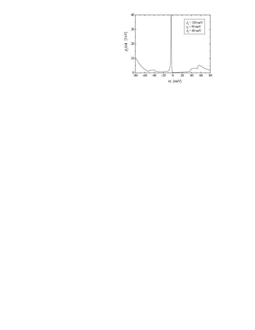
Figure 3: A typical impurity spectrum in the Kondo screened phase for given fermionic and bosonic coupling constants and for a given spin gap. The scattering potential is $V_{0}=0.2$, and the SC host is in the pure BCS state (“1”). The impurity spectral function develops a peaked structure at a characteristic Kondo energy scale $T^{\ast}$.

In the present large-$\mathcal{N}$ analysis $T_{\text{K}}$ and $T^{\ast}$ are not equivalent, i.e., they do not behave in the same manner upon approaching the transition. Nevertheless, $T^{\ast}$ can be used to characterize Kondo screening since (i) the local magnetic susceptibility changes its behavior at $T^{\ast}$ and (ii) the peaked structure at $T^{\ast}$ also appears in the conduction electron $T$-matrix as seen both in the large-$\mathcal{N}$ and the NRG calculations.cassanellofradkin ; polkovnikovSTM ; vojtabullaSTM (Note, however, that in the NRG calculations the characteristic energy scale, $T^{\ast}$, can be identified with the Kondo temperature up to a numerical factor of order unity.polkovnikovSTM ; vojtabullaSTM ) In the present work we perform a zero temperature calculation so that $T^{\ast}$ serves as a natural choice to characterize the Kondo screening. Furthermore, we associate the peaked structure in the impurity spectral function with the Zn resonance in the STM data.panBSCCO In other words, the Zn resonance is likely caused by a Kondo-like behavior of the induced effective magnetic moment with the Kondo temperature as a natural low-energy scale.

As already noted the resonance peak seen by STM does not decay monotonically with distance from the Zn site but rather oscillates, producing local minima and maxima in the DOS map. Remarkably, the four nearest neighbor Cu sites around the impurity have no DOS local maxima associated with them (in contrast to the next-nearest and next-next-nearest neighbor Cu sites).panBSCCO This non-monotonic spatial dependence cannot be naturally explained within the PS model. On the other hand, the four-site Kondo model for an impurity in a $d$-wave superconductor can capture this feature.polkovnikovSTM ; vojtabullaSTM

IV.3.2 Characteristic Kondo Energy Scale

Here we analyze how the characteristic energy scale changes with the Kondo coupling when the impurity is placed in different regions of the SC host. In Fig. 4 we show how $T^{\ast}$ depends on the Kondo coupling when a host LDOS is modified from the pure BCS to the “pseudogap” case (the corresponding LDOS are shown in Fig. 1). We see that a larger value of the Kondo coupling is required in order to screen the impurity moment in the large-gap regions (i.e., the large-gap regions have larger critical Kondo coupling, $J_{\text{Kc}}$, below which the moment is free and above which the moment is screened). In particular, for certain values of $J_{\text{K}}$ the screening is possible only in the small-gap regions and not possible in the large-gap regions. In other words, the Kondo-like impurity resonance is suppressed by going from the pure BCS to the “pseudogap” state; this is an important result which is supported by the experimental data.langBSCCO This fact cannot be explained within the PS model but naturally arises in the Kondo model.

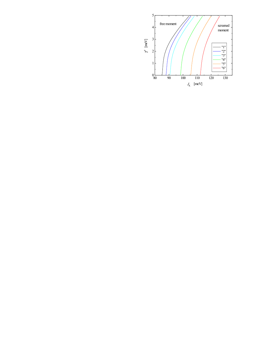
Figure 4: (color online) The characteristic energy scale as a function of the Kondo coupling for different host regions (the corresponding LDOS are given in Fig. 1). The potential scattering and the bosonic bath are absent: $V_{0}=0$, $\gamma_{0}=0$. The pure BCS state (small-gap domain) has lowest $J_{\text{Kc}}$.

Note that the values of $T^{\ast}\sim\mathcal{O}(\text{meV})$ also agree well with the Kondo temperatures estimated in NMR experiments $\sim\mathcal{O}(10\,\text{K})$.bobroff In Ref. vojtabullaSTM, it has already been shown that the presence of weak to moderate potential scattering does not change the results of the four-site fermionic Kondo model. In contrast, large values of the scattering potential induce a large DOS on the neighboring sites of the Zn impurity. As a consequence the critical Kondo coupling is strongly reduced and the Kondo scale is increased up to temperatures $\sim\mathcal{O}(100\,\text{K})$, which is in disagreement with the NMR data.bobroff On the other hand, the Kondo temperature is suppressed in the presence of the collective bosonic modes which are included in the Bose-Fermi Kondo model. In what follows we present the phase diagram of the Bose-Fermi Kondo model obtained using the large-$\mathcal{N}$ approach and also show the suppression of the Kondo screening in the presence of the collective bosonic modes.

IV.3.3 The Phase Diagram

The projection of the phase diagram onto the $J_{\text{K}}$-$\gamma_{0}$ plane is shown in Fig. 5 where the critical coupling $J_{\text{Kc}}$ is determined for different values of the spin gap and the host SC in the pure BCS state (“1”). For $\gamma_{0}=0$ we recover a fermionic pseudogap Kondo model with a finite value of $J_{\text{Kc}}$ which is, as expected, independent of the spin gap; below $J_{\text{Kc}}$ the impurity moment is free. For $\gamma_{0}\neq 0$ and $J_{\text{K}}<J_{\text{Kc}}$ we distinguish two different cases: (i) For the gapless bosonic bath, $\Delta_{\text{s}}=0$, the impurity moment is not completely free but rather placed into a bosonic fractional (fluctuating) phase.bkVBS (ii) A coupling to a gapped bosonic bath, $\Delta_{\text{s}}\neq 0$, leaves the impurity completely decoupled from both baths. Furthermore, fermionic and bosonic Kondo physics compete since the larger $\gamma_{0}$ values require larger $J_{\text{Kc}}$ in order to screen the moment. (Note that the same conclusion was reached within the RG approach for the Bose-Fermi Kondo model with $\Delta_{\text{s}}=0$.BFK1 ; BFK2 ) Also, for larger spin-gap values the bosonic bath is less effective in destroying the fermionic Kondo screening. (This fact was proposed earlier to explain the NMR data showing a suppression of the Kondo screening by underdoping.BFK1 )

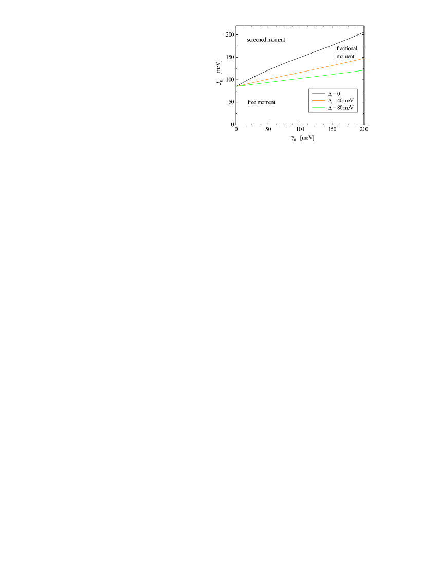
Figure 5: (color online) The projection of the phase diagram onto the $J_{\text{K}}$-$\gamma_{0}$ plane; the critical coupling $J_{\text{Kc}}$ is determined for different spin-gap values and the host SC in the pure BCS state (“1”). For $\Delta_{\text{s}}=0$ and $\gamma_{0}=0$ ($\gamma_{0}\neq 0$) there is a transition between the free (fractional) moment phase and the Kondo screened phase. For $\Delta_{\text{s}}\neq 0$ there is only a transition between the screened and the free moment phase. The potential scattering is absent, $V_{0}=0$.

In Fig. 6 we show the projection of the phase diagram onto the $J_{\text{K}}$-$\Delta_{\text{s}}$ plane. The critical Kondo coupling is determined for different values of the bosonic coupling. For $\Delta_{\text{s}}=0$ ($\Delta_{\text{s}}\neq 0$) there is a transition between the fractional (free) moment phase for $J_{\text{K}}<J_{\text{Kc}}$, and the Kondo screened phase for $J_{\text{K}}>J_{\text{Kc}}$. By increasing the spin gap the number of low-energy bosonic excitations is reduced which makes the bosonic bath less effective in destroying the Kondo screening and as a consequence $J_{\text{Kc}}$ decreases. The bosonic spin gap is doping dependent and decreases with underdoping.fong As a consequence, one expects that the bosonic bath stronger suppresses the Kondo screening in the region with lower hole doping which corresponds to the region with the larger-gap in LDOS.

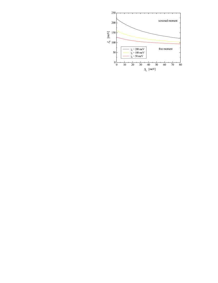
Figure 6: (color online) The projection of the phase diagram onto the $J_{\text{K}}$-$\Delta_{\text{s}}$ plane; the critical coupling $J_{\text{Kc}}$ is determined for different values of the bosonic coupling and the host SC in the pure BCS state (“1”). For $\Delta_{\text{s}}=0$ ($\Delta_{\text{s}}\neq 0$) there is a transition between the fractional (free) moment phase and the Kondo screened phase. The potential scattering is absent: $V_{0}=0$.

As mentioned above in the presence of the potential scattering the DOS on the neighboring sites of the Zn impurity increases which results in a decrease of the critical Kondo coupling. For example, for $\gamma_{0}=50$ meV and $\Delta_{\text{s}}=40$ meV and the host SC in the region “1”, we have $J_{\text{Kc}}=(101.3,\,100.4,\,97.3)$ meV for $V_{0}=(0,\,0.2,\,0.5)$ eV, respectively.

IV.3.4 Suppression of the Kondo Resonance

Here we discuss how the characteristic energy scale changes by modifying the superconducting host. Figure 7 shows the Kondo scale, $T^{\ast}$, as a function of an average energy gap $\bar{\Delta}_{0}$. The average energy gap is defined as $\bar{\Delta}_{0}=(\Delta_{-}+\Delta_{+})/2$ where the quantity $\Delta_{-}$ ($\Delta_{+}$) is the energy of the first peak below (above) the Fermi level in the host LDOS without impurity. For the pure BCS state $\bar{\Delta}_{0}$ corresponds to a superconducting gap $\Delta_{0}$ while in the “pseudogap” state one can estimate it from the LDOS shown in Fig. 1.

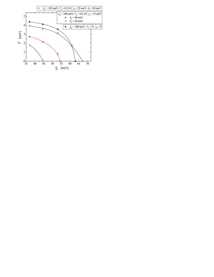
Figure 7: (color online) The characteristic energy scale as a function of the average energy gap: $J_{\text{K}}=120$ meV, $V_{0}=0.5$ eV, $\gamma_{0}=25$ meV, $\Delta_{\text{s}}=20$ meV (open squares); $J_{\text{K}}=100$ meV, $V_{0}=0.2$ eV, $\gamma_{0}=25$ meV, $\Delta_{\text{s}}=40$ meV (solid circles) and $\Delta_{\text{s}}=20$ meV (open circles); $J_{\text{K}}=100$ meV, $V_{0}=0$, $\gamma_{0}=0$ (solid squares); the lines are guides to the eye. By going from the small-gap region to the large-gap region the Kondo screening of the impurity moment vanishes.

All sets of data points in Fig. 7 indicate that the Kondo effect is more suppressed in the regions with a larger energy gap. Furthermore, the suppression of the Kondo screening is a monothonic function of the average energy gap and it is, in principle, possible to identify the maximum value of the energy gap above which the impurity resonance cannot appear in the LDOS; this agrees with the STM measurements.langBSCCO (Note that the amplitude of the Andreev resonant state in Ref. andreev, is a non-monotonic function of the energy gap; the largest resonance amplitude one obtains for intermediate gap values.) It is important to note that the Kondo energy scale $\sim\mathcal{O}(\text{meV})$ can be tuned to zero by simply modifying the host LDOS; we have shown that this is not possible in the PS model (Fig. 2). On the other hand, in the Kondo model the low-energy region of the bath LDOS is important for the Kondo effect, but through the self-consistent procedure also the LDOS away from the Fermi level influences the Kondo screening. Since the high-energy part of the bath LDOS differs significantly in small- and large-gap regions, it is natural to expect that the Kondo resonance will be affected when the host LDOS is modified.

Figure 7 also suggests that the presence of the bosonic bath additionally suppresses the Kondo screening. For the spin gap, $\Delta_{\text{s}}$, we use a constant value regardless of the specific host LDOS, i.e., regardless of doping level. We could, however, associate different spin gaps to different host LDOS since the spin gap is doping dependent;fong the underdoped regions (i.e., the regions with a larger energy gap $\bar{\Delta}_{0}$) have smaller $\Delta_{\text{s}}$. In this case, the suppression of $T^{\ast}$ with $\bar{\Delta}_{0}$ would be even more pronounced.

V Conclusions

Motivated by the question about the origin of the impurity resonance in $d$-wave SC we have compared two frequently discussed scenarios, i.e., the potential scattering model and the Kondo model. We have investigated how the STM impurity resonant state is influenced when the SC host is chosen in such a way that it resembles the nanoscale electronic inhomogeneities seen by STM.langBSCCO (i) If the impurity atom is assumed to be a pure potential scatterer we have shown within the $T$-matrix approach that the impurity resonance appears as a robust feature. The resonant state is rather insensitive to changes of the SC host. It is present in both small- and large-gap regions which is in disagreement with the experimental data. (ii) The suppression of the impurity resonance in the large-gap domains observed by STM can be naturally explained by assuming that the impurity atom gives rise to Kondo-type physics. We have used the Bose-Fermi Kondo model and the large-$\mathcal{N}$ method to show that the characteristic Kondo energy scale is affected by changing the host properties (i.e., by changing the corresponding host LDOS). The impurity resonance resulting from the Kondo screening can appear in the host small-gap regions and can be completely suppressed in the large-gap regions; this is in agreement with the STM experimental data for Zn-doped Bi₂Sr₂CaCu₂O_8+δ. Therefore, we conclude that the Kondo spin dynamics of the impurity moment is the origin of the impurity resonant state and that the pure potential scattering model is not sufficient to capture the physics of the non-magnetic impurity in $d$-wave superconductors.

- (1) E. W. Hudson, S. H. Pan, A. K. Gupta, K.-W. Ng, and J. C. Davis, Science 285, 88 (1999).
- (2) S. H. Pan, E. W. Hudson, K. M. Lang, H. Eisaki, S. Uchida, and J. C. Davis, Nature 403, 746 (2000).
- (3) K. M. Lang, V. Madhavan, J. E. Hoffman, E. W. Hudson, H. Eisaki, S. Uchida, and J. C. Davis, Nature 415, 412 (2002).
- (4) A. Sugimoto, S. Kashiwaya, H. Eisaki, H. Kashiwaya, H. Tsuchiura, Y. Tanaka, K. Fujita, and S. Uchida, Phys. Rev. B 74, 094503 (2006).
- (5) A. V. Balatsky, I. Vekhter, and J.-X. Zhu, Rev. Mod. Phys. 78, 373 (2006).
- (6) A. Yazdani, C. M. Howald, C. P. Lutz, A. Kapitulnik, and D. M. Eigler, Phys. Rev. Lett. 83, 176 (1999).
- (7) A. V. Balatsky, M. I. Salkola, and A. Rosengren, Phys. Rev. B 51, 15 547 (1995); M. I. Salkola, A. V. Balatsky, and D. J. Scalapino, Phys. Rev. Lett. 77, 1841 (1996).
- (8) W. A. Atkinson, P. J. Hirschfeld, A. H. MacDonald, and K. Ziegler, Phys. Rev. Lett. 85, 3926 (2000).
- (9) To obtain the results which are in qualitative agreement with the STM data one must include the so-called filter effect.martinfilter ; balatskyIMP
- (10) I. Martin, A. V. Balatsky, and J. Zaanen, Phys. Rev. Lett. 88, 097003 (2002).
- (11) H. Alloul, P. Mendels, H. Casalta J. F. Marucco, and J. Arabski, Phys. Rev. Lett. 67, 3140 (1991).
- (12) A. V. Mahajan, H. Alloul, G. Collin, and J. F. Marucco, Phys. Rev. Lett. 72, 3100 (1994).
- (13) M.-H. Julien, T. Fehér, M. Horvatić, C. Berthier, O. N. Bakharev, P. Ségransan, G. Collin, and J.-F. Marucco, Phys. Rev. Lett. 84, 3422 (2000).
- (14) J. Bobroff, H. Alloul, W. A. MacFarlane, P. Mendels, N. Blanchard, G. Collin, and J.-F. Marucco, Phys. Rev. Lett. 86, 4116 (2001).
- (15) A. Polkovnikov, S. Sachdev, and M. Vojta, Phys. Rev. Lett. 86, 296 (2001).
- (16) M. Vojta and R. Bulla, Phys. Rev. B 65, 014511 (2001).
- (17) M. Vojta, R. Zitzler, R. Bulla, and Th. Pruschke, Phys. Rev. B 66, 134527 (2002).
- (18) C. Howald, P. Fournier, and A. Kapitulnik, Phys. Rev. B 64, 100504(R) (2001).
- (19) S. H. Pan, J. P. O’Neal, R. L. Badzey, C. Chamon, H. Ding, J. R. Engelbrecht, Z. Wang, H. Eisaki, S. Uchida, A. K. Gupta, K.-W. Ng, E. W. Hudson, K. M. Lang, and J. C. Davis, Nature 413, 282 (2001).
- (20) K. McElroy, D.-H. Lee, J. E. Hoffman, K. M. Lang, E. W. Hudson, H. Eisaki, S. Uchida, J. Lee, and J. C. Davis, preprint cond-mat/0404005.
- (21) T. S. Nunner, B. M. Andersen, A. Melikyan, and P. J. Hirschfeld, Phys. Rev. Lett. 95, 177003 (2005).
- (22) K. McElroy, J. Lee, J. A. Slezak, D.-H. Lee, H. Eisaki, S. Uchida, and J. C. Davis, Science 309, 1048 (2005).
- (23) W. A. Atkinson, Phys. Rev. B 71, 024516 (2005).
- (24) B. M. Andersen, A. Melikyan, T. S. Nunner, and P. J. Hirschfeld, Phys. Rev. Lett. 96, 097004 (2006).
- (25) M. R. Norman, M. Randeria, H. Ding, and J. C. Campuzano, Phys. Rev. B 52, 615 (1995).
- (26) L. Zhu and Q. Si, Phys. Rev. B 66, 024426 (2002); G. Zaránd and E. Demler, ibid. 66 024427 (2002).
- (27) M. Vojta and M. Kirćan, Phys. Rev. Lett. 90, 157203 (2003).
- (28) M. Kirćan and M. Vojta, Phys. Rev. B 69, 174421 (2004).
- (29) M. Vojta, Phil. Mag. 86, 1807 (2006).
- (30) Q. Si, S. Rabello, K. Ingersent, and J. L. Smith, Nature 413, 804 (2001); M. T. Glossop and K. Ingersent, preprint cond-mat/0607566; J.-X. Zhu, S. Kirchner, R. Bulla, and Q. Si, preprint cond-mat/0607567.
- (31) S. Kirchner, L. Zhu, Q. Si, and D. Natelson, Proc. Natl. Acad. Sci. USA 102, 18824 (2005).
- (32) M. Vojta, C. Buragohain, and S. Sachdev, Phys. Rev. B 61, 15152 (2000).
- (33) H. F. Fong, P. Bourges, Y. Sidis, L. P. Regnault, J. Bossy, A. Ivanov, D. L. Milius, I. A. Aksay, and B. Keimer, Phys. Rev. B 61, 14773 (2000).
- (34) D. Withoff and E. Fradkin, Phys. Rev. Lett. 64, 1835 (1990).
- (35) C. R. Cassanello and E. Fradkin, Phys. Rev. B 53, 15079 (1996); Phys. Rev. B 56, 11246 (1997).
- (36) K. Ingersent, Phys. Rev. B 54, 11936 (1996); C. Gonzales-Buxton and K. Ingersent, ibid. 57, 14 254 (1998).
- (37) It has been shown that in the low-energy limit a possible coupling between the fermionic and the bosonic bath is forbidden by momentum conservation.bkVBS
- (38) N. Read and D. M. Newns, J. Phys. C: Solid State Phys. 16, 3273 (1983).
- (39) A. Polkovnikov, Phys. Rev. B 65, 064503 (2002).
- (40) L. Zhu, S. Kirchner, Q. Si, and A. Georges, Phys. Rev. Lett. 93, 267201 (2004).
- (41) S. Pilgram, T. M. Rice, and M. Sigrist, Phys. Rev. Lett. 97, 117003 (2006).
- (42) A. V. Chubukov, D. Pines, and J. Schmalian, preprint cond-mat/0201140.
- (43) In principle, we could introduce a -dependent factor in the expression for the self-energy to account for the difference in the nodal and antinodal regions; a suitable choice would be or . However, after the momentum summation this change would not affect the low-energy local DOS because the -dependence in the self-energy is subdominant in comparison with the linearly vanishing DOS for the bare -wave superconductor.
- (44) Experimentally it is not possible to determine the local hole doping and associate it with the certain gap value.mcelroy Nevertheless, one can measure the bulk hole doping and then associate it with the spatially averaged gap value, .