Diagrammatic determinantal quantum Monte Carlo methods:
Projective schemes and applications to the Hubbard-Holstein model

Abstract

We extend the weak-coupling diagrammatic determinantal algorithm to projective schemes as well as to the inclusion of phonon degrees of freedom. The projective approach provides a very efficient algorithm to access zero temperature properties. To implement phonons, we integrate them out in favor of a retarded density-density interaction and simulate the resulting purely electronic action with the weak-coupling diagrammatic determinantal algorithm. Both extensions are tested within the dynamical mean field approximation for the Hubbard and Hubbard-Holstein models.

I Introduction

Diagrammatic determinantal quantum Monte Carlo (DDQMC), be it the weak-coupling expansion Rubtsov05 , or hybridization expansion Werner06 approach, is emerging as the method of choice for impurity solvers Gull06 . In comparison to the Hirsch-Fye approach HirschFye86 they are continuous time methods and thereby free of Trotter errors, more efficient, and more flexible. In this article we concentrate on the weak-coupling algorithm. After a short review of our implementation of the algorithm, we show how to generalize it to projective schemes as well as to the inclusion of phonon degrees of freedom.

Projective schemes have already been implemented in the framework of the Hirsch-Fye algorithm and used in the context of dynamical mean field theories Feldbach04 ; Feldbach04_com ; Feldbach04_rep . Very similar ideas for the formulation of a projective DDQMC algorithm may be used and are reviewed in Sec. III. With the projective DDQMC, we can reproduce results of Feldbach04 at a fraction of the computational cost and access much lower projection parameters.

Phonon degrees of freedom have very recently been implemented in the hybridization formulation of the DDQMC Werner07 . Since the hybridization approach is based on the expansion in the hybridization, the inclusion of phonons relies on a Lang-Firsov transformation. In the weak coupling approach it is more convenient to integrate out the phonons in favor of a retarded interaction. The purely electronic model may then be solved efficiently within the weak coupling DDQMC. In Sec. IV we present some details of the algorithm and provide test simulations for the Hubbard-Holstein model in the dynamical mean-field theory (DMFT) approximation.

II The diagrammatic determinantal method for Hubbard interactions

Here we will briefly review the diagrammatic determinantal method for the Hubbard model

$$\hat{H}_{U}=\underbrace{-\sum_{i,j,\sigma}t_{i,j}\hat{c}^{\dagger}_{i,\sigma}\hat{c}_{j,\sigma}}_{\hat{H}_{0}}+U\sum_{i}\left(\hat{n}_{i,\uparrow}-1/2\right)\left(\hat{n}_{i,\downarrow}-1/2\right)\;,$$ (1)

where $\hat{n}_{i,\sigma}=\hat{c}^{\dagger}_{i,\sigma}\hat{c}_{i,\sigma}$ and $\hat{c}^{\dagger}_{i,\sigma}$ ($\hat{c}_{i,\sigma}$) creates (annihilates) a fermion in a Wannier state centered around site $i$ ($j$) and with $z$-component of spin $\sigma$.

As will become apparent in subsequent sections, we rewrite the Hubbard interaction as

$$\frac{U}{2}\sum_{i}\sum_{s=\pm 1}\left(\hat{n}_{i,\uparrow}-1/2-s\delta\right)\left(\hat{n}_{i,\downarrow}-1/2+s\delta\right)\;.$$ (2)

to avoid the negative sign problem at least for impurity and one-dimensional models. After carrying out the sum over the Ising spins, $s$, one recovers the original Hubbard interaction up to a constant. As will be seen below an adequate choice of $\delta$ to avoid the sign problem for a one-dimensional chain reads ${\delta=\frac{1}{2}+0^{+}}$.

A weak coupling perturbation expansion yields for the partition function:

$$\frac{Z}{Z_{0}}=\sum_{n=0}^{\infty}\left(\frac{-U}{2}\right)^{n}\int_{0}^{\beta}{\rm d}\tau_{1}\sum_{i_{1},s_{1}}\cdots\int_{0}^{\tau_{n-1}}{\rm d}\tau_{n}\sum_{i_{n},s_{n}}\prod_{\sigma}\langle\left[\hat{n}_{i_{1},\sigma}(\tau_{1})-\alpha_{\sigma}(s_{1})\right]\cdots\left[\hat{n}_{i_{n},\sigma}(\tau_{n})-\alpha_{\sigma}(s_{n})\right]\rangle_{0}\;.$$ (3)

Here, we have defined

$$\alpha_{\sigma}(s)=1/2+\sigma s\delta$$ (4)

and $\langle\bullet\rangle_{0}={\rm Tr\,}\left[e^{-\beta\hat{H}_{0}}\bullet\right]/Z_{0}$ with $Z_{0}={\rm Tr\,}\left[e^{-\beta\hat{H}_{0}}\right]$. Note that the Ising field $s$ has obtained an additional time index. The thermal expectation value is the sum over all diagrams, connected and disconnected, of a given order $n$. Using Wick’s theorem this sum can be expressed as a determinant where the entries are the Green’s functions of the non-interacting system.

$$\langle T\left[\hat{n}_{\sigma,i_{1}}(\tau_{1})-\alpha_{\sigma}(s_{1})\right]\cdots\left[\hat{n}_{\sigma,i_{n}}(\tau_{n})-\alpha_{\sigma}(s_{n})\right]\rangle_{0}=\qquad\qquad\qquad\qquad\qquad\qquad\qquad\qquad\>$$

$$\det\left(\begin{array}[]{cccc}G^{0}_{i_{1},i_{1}}(\tau_{1},\tau_{1})-\alpha_{\sigma}(s_{1})&G^{0}_{i_{1},i_{2}}(\tau_{1},\tau_{2})&\cdots&G^{0}_{i_{1},i_{n}}(\tau_{1},\tau_{n})\\ G^{0}_{i_{2},i_{1}}(\tau_{2},\tau_{1})&G^{0}_{i_{2},i_{2}}(\tau_{2},\tau_{2})-\alpha_{\sigma}(s_{2})&\cdots&G^{0}_{i_{2},i_{n}}(\tau_{2},\tau_{n})\\ \cdot&\cdot&\cdot&\cdot\\ \cdot&\cdot&\cdot&\cdot\\ \cdot&\cdot&\cdot&\cdot\\ G^{0}_{i_{n},i_{1}}(\tau_{n},\tau_{1})&G^{0}_{i_{n},i_{2}}(\tau_{n},\tau_{2})&\cdots&G^{0}_{i_{n},i_{n}}(\tau_{n},\tau_{n})-\alpha_{\sigma}(s_{n})\end{array}\right)\;,$$ (11)

with Green’s functions

$$G^{0}_{i,j}(\tau_{1},\tau_{2})=\langle T\hat{c}^{\dagger}_{i}(\tau_{1})\hat{c}_{j}(\tau_{2})\rangle_{0}\;,$$ (12)

which we have assumed to be spin independent. In the above, $T$ corresponds to the time ordering. Defining a configuration, $C_{n}$, by the $n$ Hubbard vertices, as well as the Ising spins introduced in Eq. (2)

$$C_{n}=\left\{\left[i_{1},\tau_{1},s_{1}\right]\cdots\left[i_{n},\tau_{n},s_{n}\right]\right\}\;,$$ (13)

and the sum over the configuration space by

$$\sum_{C_{n}}=\sum_{n=0}^{\infty}\int_{0}^{\beta}{\rm d}\tau_{1}\sum_{i_{1},s_{1}}\cdots\int_{0}^{\tau_{n-1}}{\rm d}\tau_{n}\sum_{i_{n},s_{n}}\;,$$ (14)

the partition function can conveniently be written as

$$\frac{Z}{Z_{0}}=\sum_{C_{n}}\left(-\frac{U}{2}\right)^{n}\prod_{\sigma}\det M_{\sigma}(C_{n})\;.$$ (15)

Here $M_{\sigma}$ is the $n\times n$ matrix of Eq. (II). Observables, $\hat{O}(\tau)$, can now be computed with

$$\langle\hat{O}(\tau)\rangle=\frac{\sum_{C_{n}}\left(-\frac{U}{2}\right)^{n}\prod_{\sigma}\det M_{\sigma}(C_{n})\langle\langle\hat{O}(\tau)\rangle\rangle_{C_{n}}}{\sum_{C_{n}}\left(-\frac{U}{2}\right)^{n}\prod_{\sigma}\det M_{\sigma}(C_{n})}\;,$$ (16)

where for $\hat{O}(\tau)=\prod_{\sigma}\hat{O}_{\sigma}(\tau)$ we have

$$\langle\langle\hat{O}(\tau)\rangle\rangle_{C_{n}}=\frac{\prod_{\sigma}\langle T\left[\hat{n}_{i_{1},\sigma}(\tau_{1})-\alpha_{\sigma}(s_{1})\right]\cdots\left[\hat{n}_{i_{n},\sigma}(\tau_{n})-\alpha_{\sigma}(s_{n})\right]\hat{O}_{\sigma}(\tau)\rangle_{0}}{\prod_{\sigma}\langle T\left[\hat{n}_{i_{1},\sigma}(\tau_{1})-\alpha_{\sigma}(s_{1})\right]\cdots\left[\hat{n}_{i_{n},\sigma}(\tau_{n})-\alpha_{\sigma}(s_{n})\right]\rangle_{0}}\;.$$ (17)

For any given configuration of vertices $C_{n}$, Wick’s theorem holds. Hence, any observable can be computed from the knowledge of the single particle Green’s function

$$\langle\langle Tc^{\dagger}_{i,\sigma}(\tau)c_{j,\sigma}(\tau_{1})\rangle\rangle_{C_{n}}=G^{0}_{i,j}(\tau,\tau_{1})\qquad\qquad\qquad$$

$$-\sum_{r,s=1}^{n}G^{0}_{i,i_{r}}(\tau,\tau_{i_{r}})\left(M_{\sigma}^{-1}\right)_{r,s}G^{0}_{i_{s},j}(\tau_{s},\tau_{1})\;.$$ (18)

Here, we have assumed that the non-interacting Green’s functions are spin independent. As a consequence of the above equation, it becomes apparent that one can measure directly the Matsubara Green’s functions. This aspect facilitates the implementation of the algorithm within the framework of dynamical mean-field theories.

II.1 Sign problem

In auxiliary field determinantal methods Assaad02 it is known that the presence of particle-hole symmetry can be used to avoid the negative sign problem. An identical statement holds for the diagrammatic determinantal method. We assume that $\hat{H}_{0}$ is invariant under the particle-hole transformation

$$c^{\dagger}_{i,\sigma}\rightarrow(-1)^{i}c_{i,\sigma}.$$ (19)

As a consequence,

$$\langle T\prod_{r=1}{n}\left[\hat{n}_{i_{r},\sigma}(\tau_{r})-\alpha_{\sigma}(s_{r})\right]\rangle_{0}=\qquad\qquad$$ (20)

$$(-1)^{n}\langle T\prod_{r=1}{n}\left[\hat{n}_{i_{r},\sigma}(\tau_{r})-\alpha_{-\sigma}(s_{r})\right]\rangle_{0}\;\;\;$$

such that ${\det M_{\uparrow}=(-1)^{n}\det M_{\downarrow}}$. A glimpse at Eq. (15) will confirm the absence of sign problem for this special case. The above results is independent on the choice of $\delta$ introduced in Eq. (2). As we will see in Sec. II.3 the algorithm is optimal at $\delta=0$. In this special case, $\det M_{\uparrow}=\det M_{\downarrow}=(-1)^{n}\det M_{\downarrow}$ such that only even values of $n$ occur in the sampling. We note that this vanishing of the weight for odd values of $n$ can be avoided by choosing a small value of $\delta$.

In one dimension and in the absence of frustrating interactions, there is no negative sign problem . The diagrammatic approach also satisfies this property, provided that we choose ${\delta=1/2+0^{+}}$. The quantity $\prod_{\sigma}\det M_{\sigma}(C_{n})$ in Eq. (15) is nothing but

$${\rm Tr\,}\Big{[}e^{-\beta\hat{H}_{0}}\prod_{\sigma}\left[\hat{n}_{i_{1},\sigma}(\tau_{1})-\alpha_{\sigma}(s_{1})\right]\Big{.}\quad\qquad\qquad$$

$$\cdots\Big{.}\left[\hat{n}_{i_{n},\sigma}(\tau_{n})-\alpha_{\sigma}(s_{n})\right]\Big{]}\Big{/}{\rm Tr\,}\Big{[}e^{-\beta\hat{H}_{0}}\Big{]}\;,$$ (21)

which we can compute within the real-space world-line approach Hirsch81 ; Assaad91 . Here, each world line configuration has a positive weight. Let us consider an arbitrary world-line configuration, and a site $(i,\tau)$ in the space-time lattice. Irrespective if this site is empty, singly or doubly occupied the expectation value of the operator ${\prod_{\sigma}\left[\hat{n}_{i,\sigma}(\tau)-\alpha_{\sigma}(s)\right]}$ will take a negative value. Recall that we have set ${\delta=1/2+0^{+}}$. Hence, for each world line configuration the expectation value of the operator ${\prod_{\sigma}\left[\left(\hat{n}_{i,\sigma}(\tau)-\alpha_{\sigma}(s_{1})\right)\cdots\left(\hat{n}_{i_{n},\sigma}(\tau_{n})-\alpha_{\sigma}(s_{n})\right)\right]}$ has a sign equal to $(-1)^{n}$. Summation over all world line configurations yields the expression in Eq. (II.1) which in turn has a sign $(-1)^{n}$. This cancels the sign of the factor $(-U/2)^{n}$ in Eq. (15), thus yielding an overall positive weight.

In the rewriting of the Hubbard term (see Eq. (2)) we have introduced a new dynamical Ising field so as to avoid the negative sign problem at least for the one-dimensional Hubbard model. Alternatively, one can choose a static Ising field and compensate for it by a redefinition of $\hat{H}_{0}$. Such a static procedure is introduced in Rubtsov05 . For the class of models considered, we have not noticed substantial differences in performance between static and dynamical choices of Ising fields. We however favor the dynamical version since it allows one to keep the SU(2) spin invariant form of the non-interacting Hamiltonian $\hat{H}_{0}$.

II.2 Monte Carlo Sampling

In principle two moves, the addition and removal of Hubbard vertices, are sufficient . In the Metropolis scheme, the acceptance ratio for a given move reads

$$P_{C\rightarrow C^{\prime}}={\rm min}\left(\frac{T^{0}_{C^{\prime}\rightarrow C}W(C^{\prime})}{T^{0}_{C\rightarrow C^{\prime}}W(C)},1\right)\;.$$ (22)

where ${T^{0}_{C^{\prime}\rightarrow C}}$ corresponds to the probability of proposing a move from configuration $C^{\prime}$ to configuration $C$ and $W(C)$ corresponds to the weight of the configuration. To add a vertex ${T^{0}_{C_{n}\rightarrow C_{n+1}}=\frac{1}{2N\beta}}$ which corresponds to the fact that one has to pick at random an imaginary time in the range $[0,\beta]$, a site $i$ in the range ${1\ldots N}$ (with $N$ the number of sites) as well as an Ising spin. The proposal probability to remove a vertex ${T^{0}_{C_{n+1}\rightarrow C_{n}}=\frac{1}{n+1}}$ corresponds to the fact that one will choose at random one of the $n+1$ vertices present in configuration $C_{n+1}$, hence

$$P_{C_{n}\rightarrow C_{n+1}} = {\rm min}\left(-\frac{U\beta N}{(n+1)}\frac{\prod_{\sigma}\det M_{\sigma}(C_{n+1})}{\prod_{\sigma}\det M_{\sigma}(C_{n})},1\right)$$

$$P_{C_{n+1}\rightarrow C_{n}} = {\rm min}\left(-\frac{(n+1)}{U\beta N}\frac{\prod_{\sigma}\det M_{\sigma}(C_{n})}{\prod_{\sigma}\det M_{\sigma}(C_{n+1})},1\right)\;.$$

Apart from the above addition and removal of vertices, we have implemented moves which flip the Ising spins at constant order $n$ as well as updates which move Hubbard vertices both in space and time.

II.3 Tests

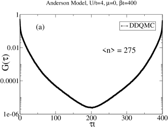
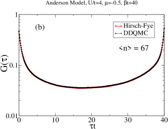
Figure 1: (Color online) Green’s function $G(\tau)$ for the Anderson model of Eq. (26). (a) Particle-hole symmetric point, $\mu=0$. To avoid the vanishing of the weight at odd values of $n$ we have used $\delta=0.1$ for this simulation. (b) Away from particle-hole symmetry $\mu=-0.5$. For this higher temperature we provide a comparison with the Hirsch-Fye algorithm with Trotter step $\Delta\tau t=0.1$. Note that in both cases we have used a $32\times 32$ square lattice to generate the non-interacting Green’s function $G^{0}(\tau)$. $\langle n\rangle$ corresponds to the average order expansion parameter.

The efficiency of the approach relies on the autocorrelation time, which has to be analyzed on a case to case basis, as well as on the average expansion order parameter. For a general interaction term $\hat{H}_{1}$ the average expansion parameter is given by

$$\langle n\rangle = \frac{1}{Z}\sum_{n}\frac{(-1)^{n}n}{n!}\int_{0}^{\beta}{\rm d}\tau_{1}\cdots\int_{0}^{\beta}{\rm d}\tau_{n}$$ (24)

$$\times\;\langle T\hat{H}_{1}(\tau_{1})\cdots\hat{H}_{1}(\tau_{n})\rangle_{0}$$

$$= \frac{-1}{Z}\sum_{m}\frac{(-1)^{m}}{m!}\int_{0}^{\beta}{\rm d}\tau_{1}\cdots\int_{0}^{\beta}{\rm d}\tau_{m}\int_{0}^{\beta}{\rm d}\tau$$

$$\times\;\langle T\hat{H}_{1}(\tau_{1})\cdots\hat{H}_{1}(\tau_{m})\hat{H}_{1}(\tau)\rangle_{0}$$

$$= -\int_{0}^{\beta}{\rm d}\tau\langle\hat{H}_{1}(\tau)\rangle\;.$$

For the Hubbard model and replacing $\hat{H}_{1}$ by the form of Eq. (2) we obtain:

$$\langle n\rangle=-\beta U\sum_{i}\left[\langle(\hat{n}_{i,\uparrow}-1/2)(\hat{n}_{i,\downarrow}-1/2)\rangle-\delta^{2}\right]\;.$$ (25)

Using the same techniques as in auxiliary field QMC methods Assaad02 the CPU costs for the calculation of the acceptance probability and the update for the addition or removal of a vertex scales as $n^{2}$. As apparent from Eq. (25) a sweep consisting of updating all $n$ vertices results in an effort of $n^{3}$. Even though in this method ${M^{-1}_{\sigma}}$ is far better conditioned than in the classic determinantal methods HirschFye86 ; Blankenbecler81 ; Assaad02 , it has to be recalculated from scratch after several updates which involves an effort of the order $n^{3}$ . Hence, because of these two limiting factors the CPU time scales as ${(\beta\,UN)^{3}}$ which is precisely the same scaling as in the Hirsch-Fye approach. Apart from the absence of Trotter errors the advantage of the method lies in a large pre-factor. In the very special case of a single impurity, $N=1$, and for a particle-hole symmetric Hamiltonian $\hat{H}_{0}$, the speedup is dramatic. Particle-hole symmetry allows one to set ${\delta=0}$ such that ${\langle n\rangle<\beta\,U/4}$. To obtain this upper bound we have set the double occupancy to zero. Hence a simulation at ${U/t=4}$ and ${\beta\,t=400}$ has a maximal average order parameter ${\langle n\rangle=400}$. In a Hirsch-Fye approach, one could opt for a Trotter step $\Delta\tau t=1/8$ and hence $3200$ Trotter slices which determines the size of the matrices involved in the simulations. Hence an underestimate of the speedup reads ${(3200/400)^{3}=512}$. Away from particle-hole symmetry, the speedup is less impressive since we have to set ${\delta=1/2+0^{+}}$ to avoid the negative sign problem. We have confirmed the above statements for the Anderson impurity model,

$$\hat{H} = \sum_{k,\sigma}(\epsilon(k)-\mu)\hat{c}^{\dagger}_{k,\sigma}\hat{c}_{k,\sigma}+\frac{V}{\sqrt{N}}\sum_{k,\sigma}\left(\hat{c}^{\dagger}_{k,\sigma}\hat{d}_{\sigma}+H.c.\right)$$ (26)

$$+U\left(\hat{d}_{\uparrow}^{\dagger}\hat{d}_{\uparrow}-1/2\right)\left(\hat{d}_{\downarrow}^{\dagger}\hat{d}_{\downarrow}-1/2\right),$$

with Hubbard interaction $U$ and hybridization $V$. Here $\hat{c}^{\dagger}_{k,\sigma}$ ($\hat{c}_{k,\sigma}$) creates (annihilates) a fermion in the conduction band at momentum $k$ with spin $\sigma$ and the dispersion relation ${\epsilon(k)=-2t(\cos(k_{x})+\cos(k_{y}))}$. The operators $\hat{d}^{\dagger}_{\sigma}$ and $\hat{d}_{\sigma}$ create, annihilates an impurity electron, respectively. Our results including comparison with the Hirsch-Fye algorithm are presented in Fig. 1.

Finally let us note that applying the method to a one-dimensional Hubbard model of length $N$, yields a very poor performance in comparison to standard finite temperature BSS auxiliary field algorithms Blankenbecler81 since those methods scale as ${\beta\,UN^{3}}$ Assaad02 .

III Generalization to projective Approaches

Projective approaches rely on the filtering out of the ground state, ${|\Psi_{0}\rangle}$ from a trial wave function $|\Psi_{T}\rangle$, which is required to be non-orthogonal to ${|\Psi_{0}\rangle}$

$$\frac{\langle\Psi_{0}|\hat{O}|\Psi_{0}\rangle}{\langle\Psi_{0}|\Psi_{0}\rangle}=\lim_{\Theta\rightarrow\infty}\frac{\langle\Psi_{T}|e^{-\frac{\Theta}{2}\hat{H}}\hat{O}e^{-\frac{\Theta}{2}\hat{H}}|\Psi_{T}\rangle}{\langle\Psi_{T}|e^{-\Theta\hat{H}}|\Psi_{T}\rangle}\;.$$

For convenience and simplicity, we will assume that ${|\Psi_{T}\rangle}$ is the ground state of $\hat{H}_{0}$, such that for a given value of $\Theta$ the right hand side of the above equation can be written as

$$\frac{\langle\Psi_{T}|e^{-\frac{\Theta}{2}\hat{H}}\hat{O}e^{-\frac{\Theta}{2}\hat{H}}|\Psi_{T}\rangle}{\langle\Psi_{T}|e^{-\Theta\hat{H}}|\Psi_{T}\rangle}\qquad\qquad\qquad\qquad\qquad$$

$$=\lim_{\beta_{0}\rightarrow\infty}\frac{{\rm Tr\,}e^{-\beta_{0}\hat{H}_{0}}e^{-\frac{\Theta}{2}\hat{H}}\hat{O}e^{-\frac{\Theta}{2}\hat{H}}}{{\rm Tr\,}e^{-\beta_{0}\hat{H}_{0}}e^{-\Theta\hat{H}}}\;.$$ (28)

With the definition ${Z_{p}={\rm Tr\,}\left[e^{-\beta_{0}\hat{H}_{0}}e^{-\Theta\hat{H}}\right]}$ and ${Z_{p,0}={\rm Tr\,}\left[e^{-(\beta_{0}+\Theta)\hat{H}_{0}}\right]}$ a weak coupling expansion yields

$$\frac{Z_{p}}{Z_{p,0}}=\sum_{n=0}^{\infty}\left(\frac{-U}{2}\right)^{n}\int_{0}^{\Theta}{\rm d}\tau_{1}\sum_{i_{1},s_{1}}\cdots\int_{0}^{\tau_{n-1}}{\rm d}\tau_{n}\sum_{i_{n},s_{n}}\prod_{\sigma}\langle\left[\hat{n}_{i_{1},\sigma}(\tau_{1})-\alpha_{\sigma}(s_{1})\right]\cdots\left[\hat{n}_{i_{n},\sigma}(\tau_{n})-\alpha_{\sigma}(s_{n})\right]\rangle_{p,0}\;,$$ (29)

where ${\langle\bullet\rangle_{p,0}={\rm Tr\,}\left[e^{-(\beta_{0}+\Theta)\hat{H}_{0}}\bullet\right]/Z_{p,0}}$. The similarity to the finite temperature algorithm is now apparent. We use Wick’s theorem to express the expectation value on the right hand side of Eq. (29) in terms of the product of two determinants. Taking the limit ${\beta_{0}\rightarrow\infty}$ we obtain

$$\langle\Psi_{T}|e^{-\Theta\hat{H}}|\Psi_{T}\rangle \equiv \lim_{\beta_{0}\rightarrow\infty}\frac{Z_{p}}{Z_{p,0}}$$ (30)

$$= \sum_{C_{n}}\left(-\frac{U}{2}\right)^{n}\prod_{\sigma}\det M_{\sigma,p}(C_{n})\;.\;\;\;\;$$

Here, the sum runs over all configurations $C_{n}$ as defined in Eq. (13) and Eq. (14). Note that $\beta$ in Eq. (14) has to be replaced by $\Theta$. The matrices $M_{\sigma,p}$ have precisely the same form as the matrices $M_{\sigma}$, but since we have taken the limit $\beta_{0}\rightarrow\infty$, the thermal non-interacting Green’s functions have to be replaced by the zero temperature ones:

$$G^{0}_{p,i,j}(\tau_{1},\tau_{2})=\langle\Psi_{T}|T\hat{c}^{\dagger}_{i}(\tau_{1})\hat{c}_{j}(\tau_{2})|\Psi_{T}\rangle\;.$$ (31)

Hence, as in the Hirsch-Fye approach, the step from a finite temperature to zero-temperature code is very easy and essentially amounts in replacing the finite temperature non-interacting Green’s functions by the zero temperature ones. However, there is an important difference concerning measurements: measurements of observables which do not commute with the Hamiltonian have to be carried out in the middle of the imaginary time interval $[0,\Theta]$ to avoid boundary effects Assaad02 .

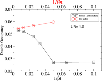
Figure 2: (Color online) DMFT calculation of the double occupancy for the half-filled Hubbard model as a function of i) temperature $1/\beta$ and ii) projection parameter $1/\Theta$. In the projective approach, observables are computed in the imaginary time range $[\Theta/4,3\Theta/4]$. This rather large measurement interval explains the slight discrepancy with the data of Ref. Feldbach04 for the projective code and at finite values of $\Theta$. However, extrapolation to $\Theta\rightarrow\infty$ where the measurement range becomes irrelevant yields results consistent with Ref. Feldbach04 .

We have tested this approach by reproducing Fig. 1 of the article Feldbach04 where the projective Hirsch-Fye algorithm was incorporated in the DMFT self-consistency cycle. Fig. 2 shows the results for the half-filled Hubbard model at $U/t=4.8$, density of states ${N(\omega)=\frac{8}{\pi W^{2}}\sqrt{W^{2}/4-\omega^{2}}}$ and band-width $W=4t$. Excellent agreement with the former Hirsch-Fye based results Feldbach04 both at finite temperatures and in the limit ${\Theta\rightarrow\infty}$ were obtained. However, the diagrammatic approach allows to access much larger projection parameters and/or lower temperatures. We refer the reader to Ref. Feldbach04 for the implementation of the projective formalism in the self-consistency cycle.

IV Application to the Hubbard-Holstein Model

Weak coupling DDQMC allows a very simple inclusion of phonon degrees of freedom. The path we follow here is to integrate out the phonons in favor of a retarded interaction, and then solve the purely electronic model with the DDQMC approach. Starting from the Hubbard-Holstein model with Einstein phonons we show how to integrate out the phonons, describe some details of the algorithm and then present results within the DMFT approximation.

IV.1 Integrating out the Phonons

The Hubbard-Holstein Hamiltonian we consider reads

$$\hat{H} = -\sum_{i,j,\sigma}t_{i,j}\hat{c}^{\dagger}_{i,\sigma}\hat{c}_{j,\sigma}+U\sum_{i}\left(\hat{n}_{i,\uparrow}-1/2\right)\left(\hat{n}_{i,\downarrow}-1/2\right)$$ (32)

$$+g\sum_{i}\hat{Q}_{i}\left(\hat{n}_{i}-1\right)+\sum_{i}\frac{\hat{P}_{i}^{2}}{2M}+\frac{k}{2}\hat{Q}_{i}^{2}\;.$$

Here, $\hat{n}_{i}=\sum_{\sigma}\hat{n}_{i,\sigma}$ and the last two terms correspond respectively to the electron-phonon coupling, $g$, and the phonon-energy. The Hamiltonian is written such that for a particle-hole symmetric band, half-filling corresponds to chemical potential $\mu=0$. Opting for fermion coherent states

$$\hat{c}_{i,\sigma}|c\rangle=c_{i,\sigma}|c\rangle\;,$$ (33)

$c_{i,\sigma}$ being a Grassmann variable, and a real space representation for the phonon coordinates

$$\hat{Q}_{i}|q\rangle=q_{i}|q\rangle\;,$$ (34)

the path integral formulation of the partition function reads

$$Z=\int\left[{\rm d}q\right]\left[dc^{\dagger}dc\right]e^{-(S_{U}+S_{\rm ep})}\;,$$ (35)

with

$$S_{U} = \int_{0}^{\beta}{\rm d}\tau\sum_{i,j,\sigma}c^{\dagger}_{i,\sigma}(\tau)\left(\delta_{i,j}\frac{\partial}{\partial\tau}-t_{i,j}\right)c_{j,\sigma}(\tau)$$

$$+\,U\sum_{i}(n_{i,\uparrow}(\tau)-1/2)(n_{i,\downarrow}(\tau)-1/2)$$

$$S_{\rm ep} = \int_{0}^{\beta}{\rm d}\tau\sum_{i}\frac{M\dot{q_{i}}^{2}(\tau)}{2}+\frac{k}{2}q_{i}^{2}(\tau)$$ (36)

$$+\,g\,q_{i}(\tau)(n_{i}(\tau)-1)\;.$$

In Fourier space,

$$q_{j}(\tau)=\frac{1}{\sqrt{\beta N}}\sum_{k,\Omega_{m}}e^{-i(\Omega_{m}\tau-kj)}q_{k,m}\;,$$ (37)

where $\Omega_{m}$ is a bosonic Matsubara frequency, the electron phonon part of the action reads

$$S_{\rm ep}=\sum_{\Omega_{m},k}\frac{M}{2}\left(\Omega_{m}^{2}+\omega_{0}^{2}\right)q^{\dagger}_{k,m}q_{k,m}+gq_{k,m}\rho^{\dagger}_{k,m}\;,$$

$$\rho^{\dagger}_{k,m}=\frac{1}{\sqrt{\beta N}}\int{\rm d}\tau\sum_{j}e^{-i(\Omega_{m}\tau-kj)}(n_{j}(\tau)-1)\,.$$ (38)

Gaussian integration over the phonon degrees of freedom leads to a retarded density-density interaction:

$$\int\left[{\rm d}q\right]e^{-S_{\rm ep}}=\quad\qquad\qquad\qquad\qquad\qquad\qquad\qquad$$

$$e^{\int_{0}^{\beta}{\rm d}\tau\int_{0}^{\beta}{\rm d}\tau^{\prime}\sum_{i,j}\left[n_{i}(\tau)-1\right]D^{0}(i-j,\tau-\tau^{\prime})\left[n_{j}(\tau^{\prime})-1\right]}\;.$$ (39)

For Einstein phonons the phonon propagator is diagonal in real space,

$$D^{0}(i-j,\tau-\tau^{\prime})=\delta_{i,j}\frac{g^{2}}{2k}P(\tau-\tau^{\prime})\;\;{\rm with}$$

$$P(\tau)=\frac{\omega_{0}}{2\left(1-e^{-\beta\omega_{0}}\right)}\left(e^{-|\tau|\omega_{0}}+e^{-(\beta-|\tau|)\omega_{0}}\right).$$ (40)

Hence the partition function of the Hubbard-Holstein model takes the form.

$$Z=\int\left[dc^{\dagger}dc\right]\times\qquad\qquad\qquad\qquad\qquad\qquad\qquad\qquad$$ (41)

$$\qquad e^{-(S_{U}-\int_{0}^{\beta}{\rm d}\tau\int_{0}^{\beta}{\rm d}\tau^{\prime}\sum_{i,j}\left[n_{i}(\tau)-1\right]D^{0}(i-j,\tau-\tau^{\prime})\left[n_{j}(\tau^{\prime})-1\right])}\;.$$

In the anti-adiabatic limit, $\lim_{\omega_{0}\rightarrow\infty}P(\tau)=\delta(\tau)$ such that the phonon interaction maps onto an attractive Hubbard interaction of magnitude $g^{2}/k$. We are now in a position to apply the DDQMC algorithm by expanding in both the retarded and Hubbard interactions.

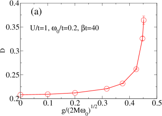
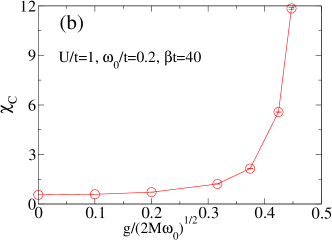
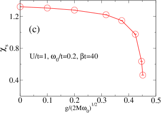
Figure 3: (a) Double occupancy, (b) local charge susceptibility and (c) local spin susceptibility for the Hubbard-Holstein model in the DMFT approximation.

.

IV.2 Formulation of DDQMC for the Hubbard-Holstein model

To avoid the minus-sign problem at least for the one-dimensional chains we rewrite the phonon retarded interaction as:

$$H_{P}(\tau) \!\!\!\!\!=-\frac{g^{2}}{4k}\int_{0}^{\beta}{\rm d}\tau^{\prime}\sum_{i,\sigma,\sigma^{\prime}}\sum_{s=\pm 1}P(\tau-\tau^{\prime})\times$$

$$\left[n_{i,\sigma}(\tau)-\alpha_{+}(s)\right]\left[n_{i,\sigma^{\prime}}(\tau^{\prime})-\alpha_{+}(s)\right].$$

For each phonon vertex, we have introduced an Ising variable: $s$. Summation over this Ising field reproduces, up to a constant, the original interaction. Since the phonon term is attractive the adequate choice of signs is ${\alpha_{+}(s)\equiv 1/2+s\delta}$, irrespective of the spin $\sigma$ and $\sigma^{\prime}$. A similar argument as presented in Sec. II.1 then guarantees the absence of a sign problem for chains. Following Eq. (2) we rewrite Hubbard term as

$$H_{U}(\tau)=\frac{U}{2}\sum_{i,s}\prod_{\sigma}(n_{i,\sigma}(\tau)-\alpha_{\sigma}(s))\;.$$ (43)

To proceed with a description of the implementation of the algorithm it is useful to define a general vertex

$$V(\tau)=\left\{i,\tau,\sigma,\tau^{\prime},\sigma^{\prime},s,b\right\}\;,$$ (44)

where $b$ defines the type of vertex at hand, Hubbard (${b=0}$) or phonon (${b=1}$). For this vertex we define a sum over the available phase phase

$$\sum_{V(\tau)}=\sum_{i,\sigma,\sigma^{\prime},s,b}\int_{0}^{\beta}{\rm d}\tau^{\prime}$$ (45)

a weight

$$w\left[V(\tau)\right]=\delta_{b,0}\frac{U}{2}-\delta_{b,1}P(\tau-\tau^{\prime})\frac{g^{2}}{4k}\;,$$ (46)

as well as

$$H \!\!\!\!\!\!\!\left[V(\tau)\right]=\delta_{b,0}\delta_{\sigma,\uparrow}\delta_{\sigma^{\prime},\downarrow}\delta(\tau-\tau^{\prime})$$

$$\left[n_{i,\uparrow}(\tau)-\alpha_{+}(s)\right]\left[n_{i,\downarrow}(\tau)-\alpha_{-}(s)\right]+$$

$$\delta_{b,1}\left[n_{i,\sigma}(\tau)-\alpha_{+}(s)\right]\left[n_{i,\sigma^{\prime}}(\tau^{\prime})-\alpha_{+}(s)\right].$$

With the above definitions, the partition function can now be written as

$$\frac{Z}{Z_{0}}=\sum_{n=0}^{\infty}(-1)^{n}\int_{0}^{\beta}{\rm d}\tau_{1}\sum_{V_{1}(\tau_{1})}w[V_{1}(\tau_{1})]\cdots\int_{0}^{\tau_{n-1}}{\rm d}\tau_{n}$$

$$\sum_{V_{n}(\tau_{n})}w\left[V_{n}(\tau_{n})\right]\langle T\hat{H}\left[V_{1}(\tau_{1})\right]\cdots\hat{H}\left[V_{n}(\tau_{n})\right]\rangle_{0}\;.$$ (48)

As for the Hubbard model, a configuration consists of a set vertices ${C_{n}=\left\{V_{1}(\tau_{1}),\ldots,V_{n}(\tau_{n})\right\}}$. For a given configuration the thermal expectation value maps onto the product of two determinants in the spin up and spin down sectors. The Monte Carlo sampling follows precisely the scheme presented in Sec. II.2, namely the addition and removal of vertices.

IV.3 Application to the Hubbard-Holstein model in the dynamical mean field approximation

We have applied the above algorithm to the Hubbard-Holstein model within the dynamical mean-field theory approximation. We use a semicircular density of states, ${N(\omega)=\frac{8}{\pi W^{2}}\sqrt{W^{2}/4-\omega^{2}}}$ with band-width ${W=4t}$. Throughout this section, we set ${U/t=1}$, ${\omega_{0}=0.2t}$, ${\mu=0}$, and use the finite temperature implementation of the algorithm at ${\beta t=40}$. The choice ${\mu=0}$ corresponds to half-filling. Fig. 3(a) plots the double occupancy, ${D=\langle n_{i,\uparrow}n_{i,\downarrow}\rangle}$ as a function of the electron-phonon coupling. To compare at best with the results of Ref. Koller04 we write the phonon coordinates in terms of bosonic operators, ${\hat{Q}=\frac{1}{\sqrt{2M\omega_{0}}}\left(\hat{a}+\hat{a}^{\dagger}\right)}$, and plot our results as a function of

$$\tilde{g}=g/\sqrt{2M\omega_{0}}\;.$$ (49)

Comparison of the results of Fig. 3(a) with those of Ref. Koller04 , show excellent agreement and a critical electron-phonon coupling for the transition to the bipolaronic insulator at ${\tilde{g}_{c}\simeq 0.45t}$.

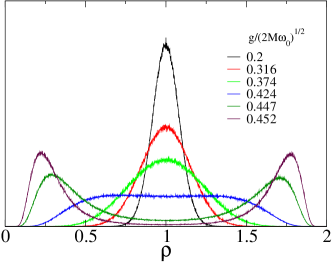
Figure 4: (Color online) The normalized histogram of the local density $\rho$ of the Hubbard-Holstein model at half-filling with ${U/t=1}$, ${\omega_{0}=0.2t}$ and ${\beta t=40}$, for several values of the electron-phonon coupling $g$.

We have equally computed the local spin and charge susceptibilities:

$$\chi_{\stackrel{{\scriptstyle C}}{{S}}}=\int_{0}^{\beta}{\rm d}\tau\langle\left[\hat{n}_{i,\uparrow}(\tau)\pm\hat{n}_{i,\downarrow}(\tau)\right]\left[\hat{n}_{i,\uparrow}\pm\hat{n}_{i,\downarrow}\right]\rangle\;.$$ (50)

As can be seen in Fig. 3(b) in the vicinity the transition local charge fluctuations grow substantially and local spin fluctuations (see Fig. 3(c)) are suppressed. The suppression of $\chi_{S}$ signals singlet pairing of polarons. The chemical potential $\mu=0$ sets the average particle number $\rho=1$ but the particle number itself oscillates strongly between an empty or doubly occupied site. This can be seen by taking histograms as shown in Fig. 4. In the vicinity of the transition a two peak structure corresponding to a doubly occupied or empty site emerges. Close to the transition it becomes increasingly hard to guarantee a symmetric histogram – corresponding to the particle-hole symmetry of the model – and the simulation ultimately freezes in the doubly occupied or empty state.

V Conclusions

We have presented two extensions of the diagrammatic determinantal method: projective schemes as well as the inclusion of phonons. In both cases we have tested successfully the approach for the Hubbard as well as for the Hubbard-Holstein models in the dynamical mean-field approximation. The inclusion of phonons is not limited to Einstein modes and in principle any dispersion relation can be easily implemented. One of the strong points of the weak-coupling DDQMC can be extended very easily to larger clusters and used as a solver for cluster extensions of dynamical mean-field theories Maier05 . The crucial issue here is the severity of the sign problem as the cluster size increases. This is an issue which would need to be answered on a case to case basis.

References

• (1) A. N. Rubtsov, V. V. Savkin, and A. I. Lichtenstein, Phys. Rev. B 72, 035122 (2005).
• (2) P. Werner, A. Comanac, L. deMedici, M. Troyer, and A. J. Millis, Phys. Rev. Lett. 97, 076405 (2006).
• (3) E. Gull, P. Werner, A. J. Millis, and M. Troyer, cond-mat/0609438 .
• (4) J. E. Hirsch and R. M. Fye, Phys. Rev. Lett. 56, 2521 (1986).
• (5) M. Feldbacher, K. Held, and F. F. Assaad, Phys. Rev. Lett. 93, 136405 (2004).
• (6) M. I. Katsnelson, Phys. Rev. Lett. 96, 139701 (2006).
• (7) M. Feldbacher, K. Held, and F. F. Assaad, Phys. Rev. Lett. 96, 139702 (2006).
• (8) P. Werner and A. J. Millis, cond-mat/0701730 .
• (9) F. F. Assaad, in Lecture notes of the Winter School on Quantum Simulations of Complex Many-Body Systems: From Theory to Algorithms., edited by J. Grotendorst, D. Marx, and A. Muramatsu. (Publication Series of the John von Neumann Institute for Computing, Jülich, 2002), Vol. 10, pp. 99–155.
• (10) J. E. Hirsch, R. L. Sugar, D. J. Scalapino, and R. Blankenbecler, Phys. Rev. B 26, 5033 (1982).
• (11) F. F. Assaad and D. Würtz, Phys. Rev. B 44, 2681 (1991).
• (12) R. Blankenbecler, D. J. Scalapino and R. L. Sugar, Phys. Rev. D 24, 2278 (1981). D. J. Scalapino and R. L. Sugar, Phys. Rev. B 24, 4295 (1981).
• (13) W. Koller, D. Meyer, Y. Ono, and A. Hewson, Euro. Phys. Lett. 66, 559 (2004).
• (14) T. Maier, M. Jarrell, T. Pruschke, and M. H. Hettler, Rev. Mod. Phys. 77, 1027 (2005).