Avalanche Size Scaling in Sheared Three-Dimensional Amorphous Solid

Abstract

We have studied the statistics of plastic rearrangement events in a simulated amorphous solid at $T=0$. Events are characterized by the energy release and the “slip volume”, the product of plastic strain and system volume. Their distributions for a given system size $L$ appear to be exponential, but a characteristic event size cannot be inferred, because the mean values of these quantities increase as $L^{\alpha}$ with $\alpha\sim 3/2$. In contrast to results obtained in 2D models, we do not see simply connected avalanches. The exponent suggests a fractal shape of the avalanches, which is also evidenced by the mean fractal dimension and participation ratio.

Athermal, or low temperature, plastic deformation of amorphous solids exhibits intermittent stress fluctuations and shear localization, in materials as diverse as metallic glasses Schuh and Nieh (2003), granular materials Miller et al. (1997), foams Pratt and Dennin (2003) and glassy polymers Haward and Young (1997). Detailed knowledge of plastic deformation mechanisms in amorphous solids, and their connection to macroscopic flow properties, however, remains elusive: While in crystals the dislocation provides a well defined starting point for estimates of flow stress, $\sigma_{f}$, in glasses there is no such easily characterizable defect. The traditional picture of deformation in amorphous solids–pioneered by Argon Argon (1979) and coworkers–is that plasticity involves collections of ‘relaxation centers’ Khonik et al. (1998) or ‘shear-transformation zones’(STZs) Falk and Langer (1998) which operate as localized centers of deformation. This picture is supported by simulations of deformation in amorphous metals Maeda and Takeuchi (1981); Srolovitz et al. (1982); Falk and Langer (1998); Malandro and Lacks (1999); Lund and Schuh (2003a, b) and observations of localized events Srolovitz et al. (1982); Zink et al. (2006).

Mean-field theories of plasticity Khonik et al. (1998); Falk and Langer (1998); Lemaître (2002) rely on this viewpoint, with the additional assumption that STZs operate somewhat independently. But the detailed nature of correlations between shear transformations is a subtle issue. Elementary shear transformations should give rise to long-range elastic displacement fields, in analogy with the transformation of elliptic Eshelby inclusions, in particular, a $1/r^{3}$ stress field due to a compact source. Models incorporating such interactions Bulatov and Argon (1994a); Baret et al. (2002) exhibit localization of deformation in patterns reminiscent of shear bands Langer (2001), suggesting that long-range elastic interactions may play an important role in the plastic response. The occurrence of shear bands in metallic glasses has been a major obstacle in the’ development of these materials for engineering applications Johnson (1999).

Even in carefully prepared samples (free of fracture-producing flaws), experimental observation of plastic deformation is often hindered by localization. In numerical simulations, however, it is possible to preserve translation-invariance and access statistical properties of plasticity in steady state. Athermal, quasi-static deformation allows further simplification of the underlying dynamics: Lacks has shown that in potential energy landscape (PEL), plastic deformation involves the destabilization of local minima along a single zero mode Malandro and Lacks (1998, 1999); Lacks (2001). The PEL point of view brought hope that elementary shear transformations could be identified with elementary transitions between minima in the PEL, as often held by STZ theories. This notion has been challenged, however, in recent simulations in two and three dimensions (2D and 3D). These show that individual plastic events present multiple substructures, which are more compact and localized Maloney and Lemaître (2004); Demkowicz and Argon (2005a). Maloney and Lemaître Maloney and Lemaître (2004) found that when visualized according to active atoms, plastic events–transitions between local minima–tended to be localized in one dimension but spread out along the other. This behavior led to an apparent scaling where the energy released in an event scaled as $L$, the linear system size.

It is essential to know whether the 2D results of Ref. Maloney and Lemaître (2004) should transfer to 3D. This is not obvious because the correlations that lead to an event taking place over an extended region may depend crucially on the power-law dependence of the elastic Green’s function which is weaker in 3D. In this Letter, we report 3D simulations of a realistic model metallic glass, undergoing athermal quasi-static shear deformation. The main novelties of our work are: (i) the dimensionality; (ii) our use of realistic interactions potentials; (iii) our use of fractal analysis to characterize the geometry of avalanches in 3D. Our main results are (1) we observe a scaling of event sizes with exponent close to 3/2; (2) visualization of typical large events indicates that the avalanches are no longer “simply connected”, partially localized avalanches, but rather are spread throughout the simulation box, with an apparent fractal shape, with mean fractal dimension close to 3/2. We note that this scaling behavior we differs from that observed in studies of crackling noise in magnets, dislocation avalanches in single-crystal plasticity Weiss and Marsan (2003) or other systems that are characterized by critical behavior which leads to power law distributions of event sizes Sethna et al. (2001). For such systems finite-size effects only influence the large-avalanche tail of the power law distribution. In our case the delocalized nature of the avalanches leads to a situation where the whole distribution scales with system size.

The simulated material is Mg_0.85Cu_0.15, which is the optimal glass-forming composition for the Mg-Cu system Sommer et al. (1980). This system is interesting because the addition of a small amount of Y makes it a bulk metallic glass with high strength and low weight Inoue et al. (1991). The interatomic potential is the effective medium theory Jacobsen et al. (1996), fitted to properties of the pure elements and intermetallic compounds obtained from experiment and density functional theory calculations. The configurations were created by cooling from a liquid state above the melting temperature down to T=0, using constant temperature and pressure molecular dynamics. Details of the potential and of the cooling process may be found in Bailey et al. (2004); the cooling rate for the systems studied here was about $10^{11}$Ks^-1. Periodic boundary conditions were used both in cooling and in the deformation simulations described below. Five system sizes were studied, containing 864, 2048, 4000, 8788 and 16384 atoms, with $L=26$Å, 35Å, 44Å, 57Å and 70Å, respectively. Ten independent configurations were produced for all sizes, except only one 16384-atom system.

The systems were deformed in pure shear by a variation of the standard procedure of straining the entire system homogeneously in small increments followed by energy-minimization. In the so-called quasi-static limit, the system continuously follows deformation-induced changes in local minima Malandro and Lacks (1998, 1999); this protocol is meant to capture the asymptotic trajectory in this limit. During homogeneous strains, as well as relaxing the atomic positions, components of strain apart from the one being controlled were also relaxed. In particular this means that the hydrostatic pressure was always zero. To observe scaling it is important to be close to the quasi-static limit and therefore to have a strict tolerance for minimization Maloney and Lemaître (2004); we used 10^-6eV/Å for the maximum force and 10^-6eV/Å${}^{3}=0.16$ MPa for the maximum (relaxable) stress. The homogeneous strain was applied by multiplying the simulation box vectors by a shear strain matrix at each step, with a strain size of $\Delta\epsilon=0.0005$. Here $\epsilon$ is an off-diagonal component of the strain, not the engineering strain. The total strain at any point in the deformation history is the number of steps times 0.0005. The total amount of deformation imposed was $\sim$100%. The use of periodic boundaries and the small sizes prevent any kind of macroscopic localization being observed even at such large strains.

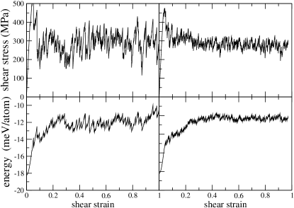
Figure 1: Stress and energy versus strain for 2048- (left) and 16384-atom (right) systems.

Examples of stress-strain curves are shown in Fig. 1. The behavior is very similar to that observed in other simulations in 2D and 3D Maloney and Lemaître (2004); Malandro and Lacks (1998, 1999): an initial linear elastic regime, followed by the onset of plasticity manifested as abrupt drops. After about 30% strain a steady state has been reached (note in particular the energy of the 16384-atom system). The stress averaged over the steady-state part of the curve, $\sigma_{f}$, is about 280 MPa, independent of $L$.

The stress- and energy-drops define distinct plastic “events”. These do not necessarily correspond to the elementary units of plastic deformation, as mentioned above; a complete event is an avalanche of sub-events. Defining subevents in a useful way is problematic in practice, hence in order to stick with meaningful and well-defined quantities, we study complete events.

We have analyzed the events in the stress and energy curves by assigning to each event two quantities. The energy and stress drops are defined relative to the values they would be expected to have given continued elastic behavior. Thus we have $\Delta\sigma_{drop}=\sigma_{i}+2\mu\Delta\epsilon-\sigma_{i+1}$, where $\mu$ is the shear modulus (determined as half the slope of the stress-strain curve), and $\Delta E_{drop}=E_{i}+V_{i}\sigma_{i}\Delta\epsilon-E_{i+1}$, where $V_{i}$ is the system volume. $\Delta E_{drop}$ ($\Delta\sigma_{drop}$) is positive if there is a drop in stress (energy). For some very small stress drops, the apparent energy drop is negative, due to finite resolution implied by a finite $\Delta\epsilon$. We count events with $\Delta\sigma_{drop}$ greater than a cutoff $\Delta\sigma_{min}$ and $\Delta E_{drop}>0$. Our scaling analysis is based on the distributions of $\Delta E_{drop}$ and a quantity proportional to $\Delta\sigma_{drop}$, that we call the slip volume, $V_{slip}\equiv V\Delta\sigma_{drop}/2\mu=V(\Delta\epsilon-(\sigma_{i+1}-\sigma_{i})/2\mu)=V(\Delta\epsilon-\Delta\epsilon_{el})=V\Delta\epsilon_{pl}$, where $\Delta\epsilon_{el}$ ($\Delta\epsilon_{pl}$) is elastic (plastic) strain. The significance of $V_{slip}$ can be understood by supposing first that the plastic slip associated with an event is confined to a localized region of space, whose size had a narrow distribution independent of $L$. If the slip is characterized as a displacement $d$ over an area $A$, then $\epsilon_{pl}=Ad/V$ and $V_{slip}=Ad$. If an event involved $m$ such elementary shear transformations the resulting $V_{slip}$ would be $\sim mAd$, and thus a measure of the number of elementary transformations which contribute to the macroscopic stress relaxation. The cutoff $\Delta\sigma_{min}$ is chosen so that the minimum $V_{slip}$ is independent of $L$ and equal to 5ų.

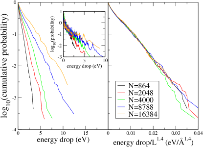
Figure 2: (Color online) Left, cumulative probability distribution of $\Delta E_{drop}$ in plastic events for different system sizes. Right, cumulative probability distribution of $\Delta E_{drop}/L^{1.4}$. Inset, probability distribution of $\Delta E_{drop}$.

In Figs. 2 and 3 are shown cumulative distributions $C(x)$ of $\Delta E$ and $V_{slip}$, where $C(x)=\int_{x}^{\infty}P(x^{\prime})dx^{\prime}$, and $P(x)$ is the probability distribution. The advantage of using $C(x)$ is that it yields a much smoother curve, while no information is lost through binning. Furthermore, for power-law or exponential behavior of $P(x)$ at large $x$, $C(x)$ maintains this behavior (with the exponent changing by one in the case of a power-law). The insets show $P(x)$, which involves a binning procedure and result in noisy curves. The $C(x)$ curves are almost linear (with perhaps some downward curvature) in these semi-log plots, suggesting that the distributions are roughly exponential. The inverse-slopes, and hence the mean values, however, systematically increase with $L$, so they cannot be associated with a characteristic event size independent of $L$. If these quantities are scaled by $L^{1.4}$ and $L^{1.6}$, respectively, the C(x) curves collapse quite well onto master curves, as shown in the right panels of Figs. 2 and 3. Changing the exponent by 0.1 produces a slightly worse collapse in both cases. The means of $\Delta E$ and $V_{slip}$ scale as $L^{1.43\pm 0.03}$ and $L^{1.63\pm 0.04}$, respectively; these exponents are consistent with the scaling collapses.

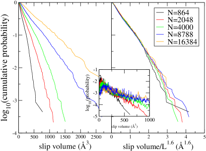
Figure 3: (Color online) Left, cumulative probability distribution of $\Delta V_{slip}$ in plastic events for different system sizes. Right, cumulative probability distribution of $\Delta V_{slip}/L^{1.6}$. Inset, probability distribution of $\Delta V_{slip}$.

Ref. Maloney and Lemaître (2004) interpreted the linear scaling with $L$ in terms of the geometrical structure of the events: they tended to be extended in one dimension, in the form of slip lines passing through the simulation cell. Extrapolating their results to 3D, one might expect planar events, scaling as $L^{2}$. This is excluded by our results. If the connection between the observed scaling of event distributions and the geometry of events is to be trusted, we can tentatively interpret the $L^{3/2}$ scaling as reflecting a fractal geometry of the avalanches, somewhere between string-like and planar. Of course, the scaling of the form $L^{3/2}=V^{1/2}$ is very reminiscent of a central limit theorem—the variance in the extensive quantities $E$ and $V\sigma$ should go like $V$ (or $N$), and $\overline{\Delta E}$ and $\overline{\Delta\sigma}$ correspond to the square root, the standard deviation. Note that the results of Ref. Maloney and Lemaître (2004) are also consistent with this interpretation, since in two dimensions $L$ is the square root of the system size. A central limit interpretation of this scaling would suggest that contributions from different parts of the system somehow add up in an uncorrelated way. The clear change in event size distribution with system size indicates that the events are spatially delocalized and in this way the resulting energy and stress drops certainly result from contributions from different parts of space. But within such a “random-noise” interpretation with uncorrelated contributions from different parts of space one would expect that the atoms participating in the event would be more or less equally distributed over space. We shall see now that this is not the case.

To study the geometrical structure of events, we need to define a measure of which atoms take part in an event. We choose to consider the atom displacements that take place during minimization $d_{i}\equiv|\Delta\vec{r}_{i}|$. Rather than impose an arbitrary cut-off to identify participating atoms, we use the participation ratio $P=(\sum_{i}d_{i}^{2})^{2}/(N\sum_{i}d_{i}^{4})$, where $N$ is the number of atoms. $P=1$ for an event where all the $d_{i}$ are equal and $1/N$ for one where a single atom moves; thus it is the effective fraction of participating atoms. In the left panel of Fig. 4 we show distributions of $P$ for different $L$, as well as the means. The mean value of $P$ is well fit by a power-law with exponent -1.44$\pm$0.03. To compare with the scaling of the extensive quantities $\Delta E$ and $V_{slip}$, we should consider $VP=L^{3}P$, or add three to the exponent. This gives 1.56, close to the $V_{slip}$ exponent, implying a similar scaling for two measures of events which may both be considered “geometrical” in a sense—we saw above that $V_{slip}$ is related to the amount of plastic strain at the boundaries that an event causes.

Given $P$ for an event, we define the set of set of participating atoms as those whose $d_{i}$ is in the top $P$ of the population. This defines the “mobile” atoms without an arbitrary cut-off. We then define the fractal dimension $D_{F}$ of the set in the usual box-counting way: Taking a box which contains all of the atoms, we divide the box by increasing powers of two (in all directions) and count how many boxes $N_{b}$ for a given divisor $d$ are required to contain all atoms in the subset. $D_{F}$ is determined as the best-fit slope on a plot of $log(N_{b})$ versus $log(d)$, assuming the data lie on a straight line. Typically four points are available for the fit. The data generally exhibit a noticeable downward curvature, so the interpretation of a fractal geometry should not be taken too literally. Even so, it is interesting that the average $D_{F}$ computed this way indeed gives the value 1.6$\pm 0.05$, independent of system size and close to the exponents determined from $V_{slip}$ and $P$; distributions of $D_{F}$ are shown in the right hand panel of Fig. 4. These observations support the idea that non-local plastic events can still be viewed as sums of similar elementary events, probably like elementary shear transformations. These sub-events organize in space along a fractal-like structure, and therefore must be strongly correlated. This suggests that mean-field approaches, such as the STZ theoryFalk and Langer (1998), may be incomplete.

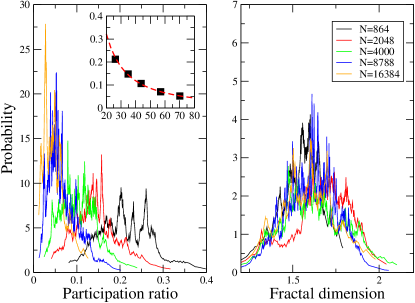
Figure 4: (Color online) Left, distribution of participation ratios $P$ for different system sizes $L$. Inset, the mean $P$ versus $L$ together with a power law fit with exponent -1.44. Right, distribution of apparent fractal dimension of participating atoms.

In summary we have observed a clear signature of a $\sim$3/2 scaling of event sizes with system size, and presented evidence that this can be attributed to a fractal-like shape of the events. The range of system sizes is not large, but the statistics are good. It is interesting to speculate whether there is a relation between the events seen in low temperature deformation and those in a supercooled liquid near the glass transition. The latter are known to exhibit strong spatial correlations; a recent attempt to infer a fractal dimension for individual clusters Vollmayr-Lee and Zippelius (2005) yielded a value of 1.8—not close enough to 1.5 to suggest an obvious connection, but enough perhaps to speculate that the dynamics changes in a smooth way upon going from high-$T$, zero stress to zero-$T$, high stress. Finally we mention the interesting question of how finite strain rates and temperatures cut off the scaling, and whether a length scale emerges from this cutting off, which could be connected to, for example, the observed width of shear bands (10–20 nm).