Feedback cooling of a cantilever’s fundamental mode below 5 mK

Abstract

We cool the fundamental mechanical mode of an ultrasoft silicon cantilever from a base temperature of 2.2 K to $2.9\pm 0.3$ mK using active optomechanical feedback. The lowest observed mode temperature is consistent with limits determined by the properties of the cantilever and by the measurement noise. For high feedback gain, the driven cantilever motion is found to suppress or “squash” the optical interferometer intensity noise below the shot noise level.

Feedback control of mechanical systems is a well-established engineering discipline which finds applications in diverse areas of physics, from the stabilization of large cavity mirrors used in gravitational wave detectors Abbott:2004 to the control of tiny cantilevers in atomic force microscopy Albrecht:1990 ; Mertz:1993 ; Garbini:1996 ; Bruland:1998 ; Weld:2006 . Recently, the prospect of cooling a mechanical resonator to its quantum ground state has spurred renewed interest in the damping of oscillators through both active feedback Kleckner:2006 and passive back-action effects Naik:2006 ; Gigan:2006 ; Arcizet:2006 . Motivated by the ability to make ever smaller mechanical devices and ever more sensitive detectors of motion, researchers are pushing into a regime in which collective vibrational motion should be quantized Schwab:2005 . In combination with conventional cryogenic techniques, the cooling of a single mechanical mode using feedback may provide an important step towards achieving the quantum limit in a mechanical system. Here we demonstrate the feedback cooling of an ultrasoft silicon cantilever to below 5 mK starting from a base temperature as high as 4.2 K. Starting from this temperature, the vibrational mode of the oscillator is cooled near the level of the measurement noise, which sets a fundamental limit on the cooling capacity of feedback damping. In the future, minimizing such noise may be key to achieving single-digit mode occupation numbers.

We study the fundamental mechanical mode of two $120\times 3\times 0.1$-$\mu$m single-crystal Si cantilevers of the type shown in Fig. 1(b). The ends of the levers are designed with a $2\times 15$-$\mu$m mass which serves to suppress the motion of flexural modes above the fundamental Chui:2003 . Cantilevers 1 and 2 have resonant frequencies of 3.9 and 2.6 kHz respectively due to the difference in mass of the samples which have been glued to their ends. The sample on cantilever 1 is a 0.1-$\mu$m³ particle of SmCo while the sample on cantilever 2 is a 50-$\mu$m³ particle of CaF₂ crystal. Both samples are not related to the work presented here aside from the added mass which they contribute. The oscillators’ spring constants are both determined to be $k=86$ $\mu$N/m through measurements of their thermal noise spectra at several different base temperatures. Each cantilever is mounted in a vacuum chamber (pressure $<1\times 10^{-6}$ torr) at the bottom of a dilution refrigerator which has been isolated from environmental vibrations. The motion of the lever is detected using laser light focused onto a 10-$\mu$m-wide paddle near the mass-loaded end and reflected back into an optical fiber interferometer Rugar:1989 . 100 nW of light are incident on the lever from a temperature-tuned 1550-nm distributed feedback laser diode Bruland:1999 . The interferometric cantilever position signal is sent through a differentiator circuit and a variable electronic gain stage back to a piezoelectric element which is mechanically coupled to the cantilever, as shown schematically in Fig. 1(a). The overall bandwidth of the feedback is controlled by bandpass filters. For negative gain, this feedback loop has the effect of producing a damping force on the cantilever proportional to the velocity of its oscillatory motion.

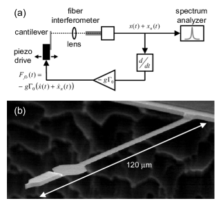
Figure 1: (a) Schematic diagram of the experimental setup and (b) scanning electron micrograph of a representative Si cantilever.

For frequencies in the vicinity of the fundamental mode resonance, the motion of a cantilever is well approximated by

$$m\ddot{x}+\Gamma_{0}\dot{x}+kx=F_{th}-g\Gamma_{0}\left(\dot{x}+\dot{x}_{n}\right),$$ (1)

where $x(t)$ is the displacement of the oscillator as a function of time, $\Gamma_{0}$ is its intrinsic dissipation, $k=m{\omega_{0}}^{2}$ is its spring constant, $m$ is the oscillator’s effective mass, $\omega_{0}$ is its angular resonance frequency, $F_{th}(t)$ is the random thermal Langevin force, and $x_{n}(t)$ is the measurement noise on the displacement signal. The dissipation can be written in terms of $m$, $\omega_{0}$, and the oscillator’s intrinsic quality factor $Q_{0}$ according to $\Gamma_{0}=m\omega_{0}/Q_{0}$.

Given the equation of motion in (1) and considering frequency components of the form $\hat{F}_{th}(\omega)e^{i\omega t}$ and $\hat{x}_{n}(\omega)e^{i\omega t}$, the frequency response of the oscillator is

$$\hat{x}(\omega)=\frac{\frac{1}{m}\hat{F}_{th}(\omega)-ig\frac{\omega_{0}\omega}{Q_{0}}\hat{x}_{n}(\omega)}{\left({\omega_{0}}^{2}-\omega^{2}\right)+i(1+g)\frac{\omega_{0}\omega}{Q_{0}}}.$$ (2)

For random excitations where $F_{th}(t)$ and $x_{n}(t)$ are uncorrelated, we can then determine the spectral density of both the oscillator’s actual displacement $x$,

$$S_{x}(\omega)= \left[\frac{1/m^{2}}{\left({\omega_{0}}^{2}-\omega^{2}\right)^{2}+\left(1+g\right)^{2}{\omega_{0}}^{2}\omega^{2}/{Q_{0}}^{2}}\right]S_{F_{th}}$$ (3)

$$+\left[\frac{g^{2}{\omega_{0}}^{2}\omega^{2}/{Q_{0}}^{2}}{\left({\omega_{0}}^{2}-\omega^{2}\right)^{2}+\left(1+g\right)^{2}{\omega_{0}}^{2}\omega^{2}/{Q_{0}}^{2}}\right]S_{x_{n}},$$

and of its measured displacement $x+x_{n}$,

$$S_{x+x_{n}}(\omega)= \left[\frac{1/m^{2}}{\left({\omega_{0}}^{2}-\omega^{2}\right)^{2}+\left(1+g\right)^{2}{\omega_{0}}^{2}\omega^{2}/{Q_{0}}^{2}}\right]S_{F_{th}}$$ (4)

$$+\left[\frac{\left({\omega_{0}}^{2}-\omega^{2}\right)^{2}+{\omega_{0}}^{2}\omega^{2}/{Q_{0}}^{2}}{\left({\omega_{0}}^{2}-\omega^{2}\right)^{2}+\left(1+g\right)^{2}{\omega_{0}}^{2}\omega^{2}/{Q_{0}}^{2}}\right]S_{x_{n}}.$$

Here $S_{x_{n}}$ is the spectral density of the measurement noise $x_{n}$ and $S_{F_{th}}$ is the white spectral density of the thermal noise force $F_{th}$. According to the fluctuation dissipation theorem, the noise force $S_{F_{th}}$ depends on the cantilever dissipation and is given by $S_{F_{th}}=4\Gamma_{0}k_{B}T$, where we are using a single-sided convention for the spectral density.

We define the mode temperature of the cantilever according to the equipartition theorem as $T_{\text{mode}}=k\left\langle x^{2}\right\rangle/k_{B}$ and calculate $\left\langle x^{2}\right\rangle$ according to $\left\langle x^{2}\right\rangle=(1/2\pi)\int_{0}^{\infty}{S_{x}(\omega)d\omega}$. Using (3) and assuming that $S_{x_{n}}$ is independent of $\omega$, we find

$$T_{\text{mode}}=\frac{T}{1+g}+\frac{k\omega_{0}}{4k_{B}Q_{0}}\left(\frac{g^{2}}{1+g}\right)S_{x_{n}},$$ (5)

where $T$ is the bath temperature and $k_{B}$ is the Boltzmann constant.

In the limit of small gain ($g<<1$), the effect of measurement noise on the oscillator displacement can be ignored and the oscillator power spectrum is obtained by simply subtracting the measurement noise floor from the measured spectrum: $S_{x}(\omega)=S_{x+x_{n}}(\omega)-S_{x_{n}}$. The same is true for large gain as long as the noise is well below the measured displacement power (more precisely, $S_{x_{n}}<<\frac{{Q_{0}}^{2}}{g^{2}k^{2}}S_{F_{th}}$). In both cases the mode temperature is proportional to the integrated area between the measured spectrum and the noise floor and reduces to the familiar $T_{\text{mode}}=\frac{T}{1+g}$ Kleckner:2006 . Increasing the damping gain lowers the mode temperature leading to “feedback cooling” or “cold damping” of the oscillator.

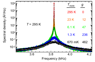
Figure 2: (Color) Measured spectral density $S_{x+x_{n}}$ of cantilever 1 for different feedback gains $g$ as it is cooled from a base temperature $T=295$ K. Colored data points correspond to the mode temperatures (with an error of $\pm 10$%) and gains of the same color shown to the right. Solid lines are fits to the data using (4).

The feedback cooling of cantilever 1 from a base temperature of 295 K falls in this limit and is shown in Fig. 2. At this temperature $Q_{0}=16,000$. As the gain increases, the mode temperature decreases down to $T_{\text{mode}}=670\pm 70$ mK for $g=462$. Even at the highest gain, the measurement noise is well below the observed thermal noise. Therefore, the temperature of the fundamental lever mode is well determined by the area between the observed peak and the noise floor. The mode temperatures shown in Fig. 2 are equal within the error whether they are calculated by simply integrating the area under the observed spectra or whether the spectra are fit using (4) and the extracted parameters are substituted in (5). The fits, which are shown as solid lines in Fig. 2, involve three free parameters: $\omega_{0}$, $g$, and $S_{x_{n}}$.

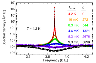
Figure 3: (Color) Measured spectral density $S_{x+x_{n}}$ of cantilever 1 for different feedback gains $g$ as it is cooled from a base temperature $T=4.2$ K. Colored data points correspond to the mode temperatures (with an error of $\pm 10$%) and gains of the same color shown to the right. Solid lines are fits to the data using (4).

When we cool cantilever 1 by feedback from a base temperature of 4.2 K, where $Q_{0}=44,200$, this approximation is no longer valid. Starting at $g\simeq 300$, the values of $T_{\text{mode}}$ calculated from simple integration of the spectrum above the noise floor begin to deviate from the more accurate values given by (5). Increasing the gain further, as shown in Fig. 3, pushes the observed thermal noise spectra down to the level of the measurement noise and beyond.

The two spectra showing a dip below the white noise floor are clear deviations from the low gain, low noise approximation; calculating the mode temperature through integration would result in unphysical negative values. Here the feedback loop counteracts intensity fluctuations in the light field by exciting the cantilever rather than by damping it. In our experiment, these intensity fluctuations are due to the shot noise of the laser field, i.e. we are operating in the limit where $S_{x_{n}}$ is dominated by the photon shot noise. From fits to the spectra, we find $\sqrt{S_{x_{n}}}\simeq 10^{-2}$ Å$/\sqrt{\text{Hz}}$. When $S_{x_{n}}$ is limited by shot noise, as in our case, its suppression by feedback is known as intensity noise “squashing” inside an optoelectronic loop Buchler:1999 ; Sheard:2005 ; Bushev:2006 .

In the high gain regime ($g>300$) of Fig. 3, we must consider the full effect of measurement noise on (4) and (3) in order to extract the actual motion of the lever. As shown in Fig. 4, the actual vibrational spectrum of lever 1 deviates from the measured spectrum as it approaches the measurement noise. Here, the limits of feedback cooling have been reached as measurement noise sent back to the piezoelectric actuator acts to heat the lever’s vibrational mode.

We observe similar behavior from cantilever 2 starting at a lower base temperature. In this case, the experimental apparatus is cooled to 250 mK. Measurement of the lever’s thermal noise spectrum, however, reveals that its base temperature reaches only 2.2 K with $Q_{0}=55,600$. This discrepancy is due to heating of the Si cantilever through the absorption of light from the interferometer laser. As shown in Fig. 5, by applying feedback cooling at this base temperature, we achieve a minimum fundamental mode temperature of $2.9\pm 0.3$ mK before $T_{\text{mode}}$ starts increasing as a function of $g$.

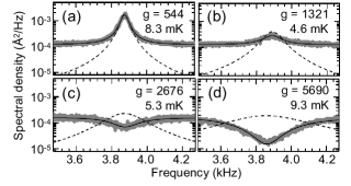
Figure 4: Suppression of the thermal noise of cantilever 1 down to and below the measurement noise. Gray points represent the observed interferometer signal $S_{x+x_{n}}$ with the lever at a base temperature of $T=4.2$ K, solid lines are fits to this data using (4), and dashed lines are the corresponding spectra of the actual cantilever motion $S_{x}$ as defined in (3).

As implied by (5) and shown in Fig. 6, the measurement noise floor sets a minimum achievable mode temperature for $g>>1$:

$$T_{\text{mode, min}}=\sqrt{\frac{k\omega_{0}T}{k_{B}Q_{0}}S_{x_{n}}}.$$ (6)

For cantilever 2 at $T=2.2$ K, we calculate $T_{\text{mode, min}}=2.6$ mK, which is close to the observed minimum temperature of $2.9\pm 0.3$ mK. A more complex expression could be written for $T_{\text{mode, min}}$ if the techniques of optimal control were used to cool the lever rather than simple velocity-proportional damping Garbini:1996 ; Bruland:1998 . For our experimental parameters, optimal control does not provide any further reduction in $T_{\text{mode, min}}$. We calculate, however, that in the low noise limit ($\sqrt{S_{x_{n}}}<10^{-4}$ Å$/\sqrt{\text{Hz}}$), it could achieve lower mode temperatures than velocity-proportional damping.

The minimum temperature in (6) immediately implies a minimum mode occupation number $N_{\text{mode, min}}=\frac{1}{\hbar}\sqrt{\frac{kk_{B}T}{\omega_{0}Q_{0}}S_{x_{n}}}$. In our case, the lowest achieved mode occupation is $N\simeq 2.3\times 10^{4}$ and $N_{\text{mode, min}}=2.1\times 10^{4}$. Since for a cantilever $\frac{k}{\omega_{0}}\propto\frac{t^{2}w}{l}$, where $l$, $w$, and $t$ are its length, width, and thickness, $N_{\text{mode, min}}\propto t\sqrt{\frac{wT}{lQ_{0}}S_{x_{n}}}$. Therefore, if low occupation numbers are to be achieved by feedback cooling, the cantilevers employed should be long and thin, have high quality factors and the measurement should be done at low base temperature with low measurement noise. The geometry of our ultra-soft cantilevers is well suited to minimize $N_{\text{mode, min}}$. It appears, therefore, that the most likely way to achieve further reductions in $N_{\text{mode, min}}$ is to reduce the measurement noise, either by using better optical interferometry or by employing a detector of cantilever motion with intrinsically higher resolution, such as a single electron transistor (SET). SETs have recently achieved $\sqrt{S_{x_{n}}}\sim 10^{-5}$ Å$/\sqrt{\text{Hz}}$ Knobel:2003 ; LaHaye:2004 ; Naik:2006 . High-frequency doubly clamped resonators cooled cryogenically below 50 mK have achieved occupation numbers down around 25 without feedback LaHaye:2004 ; Naik:2006 .

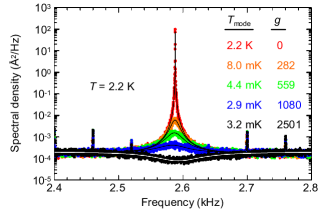
Figure 5: (Color) Measured spectral density $S_{x+x_{n}}$ of cantilever 2 for different feedback gains $g$ as it is cooled from a base temperature $T=2.2$ K. Colored data points correspond to the mode temperatures (with an error of $\pm 10$%) and gains of the same color shown to the right. Solid lines are fits to the data using (4).

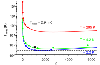
Figure 6: (Color) $T_{\text{mode}}$ of our Si cantilevers as a function of feedback gain $g$. Solid lines show $T_{\text{mode}}$ in (5) for the experimental parameters and the points represent $T_{\text{mode}}$ extracted from three-parameter fits of (3) to spectra including those shown in Figs. 2-5. Lines and points are color coded to correspond to the colored base temperature labels. The dashed line indicates $T_{\text{mode, min}}=2.6$ mK for cantilever 2 at $T=2.2$ K.

It is worth noting that the type of feedback cooling discussed here may be applicable to nanoelectromechanical systems in sensing applications. It was shown recently that as nanomechanical resonators shrink in size, their dynamic range decreases Postma:2005 ; Kozinsky:2006 . This effect is due to a combination of a decrease in the onset of nonlinearity and an increase in the thermomechanical noise with decreasing size. A resonator’s dynamic range can at least be partially recovered through feedback cooling, which reduces the thermal noise amplitude.

Finally, optimized feedback cooling may find use in the realization of a type of magnetic resonance force microscopy which detects nuclear magnetic resonance at the Larmor frequency Sidles:1992 . Such a scheme strongly couples the cantilever thermal noise to the nuclear spins and has the side-effect of dramatically increasing the nuclear spin relaxation rate. Feedback cooling could be used both to control this lever-induced relaxation and to dramatically reduce the temperature of the nuclear spin system.

- (1) B. Abbott et al., Phys. Rev. D 69, 122001 (2004).
- (2) T. R. Albrecht, P. Grütter, D. Horne, and D. Rugar, J. Appl. Phys. 69, 668 (1990).
- (3) J. Mertz, O. Marti, and J. Mlynek, Appl. Phys. Lett. 62, 2344 (1993).
- (4) J. L. Garbini, K. J. Bruland, W. M. Dougherty, and J. A. Sidles, J. Appl. Phys. 80, 1951 (1996); K. J. Bruland, J. L. Garbini, W. M. Dougherty, and J. A. Sidles, J. Appl. Phys. 80, 1959 (1996).
- (5) K. J. Bruland, J. L. Garbini, W. M. Dougherty, and J. A. Sidles, J. Appl. Phys. 83, 3972 (1998).
- (6) D. M. Weld and A. Kapitulnik, Appl. Phys. Lett. 89, 164102 (2006).
- (7) D. Kleckner and D. Bouwmeester, Nature 444, 75 (2006).
- (8) A. Naik et al., Nature 443, 193 (2006).
- (9) S. Gigan et al., Nature 444, 67 (2006).
- (10) O. Arcizet et al., Nature 444, 71 (2006).
- (11) K. C. Schwab and M. L. Roukes, Phys. Today 58, No. 7, 36 (2005).
- (12) B. W. Chui et al., Technical Digest of the 12th International Conference on Solid-State Sensors and Actuators (Transducers ’03), (IEEE Boston, MA, 2003), p. 1120.
- (13) D. Rugar, H. J. Mamin, and P. Guethner, Appl. Phys. Lett. 55, 2588 (1989).
- (14) K. J. Bruland et al., Rev. Sci. Inst. 70, 3542 (1999).
- (15) B. C. Buchler et al., Opt. Lett. 24, 259 (1999).
- (16) B. S. Sheard et al., IEEE J. Quant. Elec. 41, 434 (2005).
- (17) P. Bushev et al., Phys. Rev. Lett. 96, 043003 (2006).
- (18) R. G. Knobel and A. N. Cleland, Nature 424, 291 (2003).
- (19) M. D. LaHaye, O. Buu, B. Camarota, K. C. Schwab, Science 304, 74 (2004).
- (20) H. W. Ch. Postma, I. Kozinsky, A. Husain, and M. L. Roukes, Appl. Phys. Lett. 86, 223105 (2005).
- (21) I. Kozinsky, H. W. Ch. Postma, I. Bargatin, and M. L. Roukes, Appl. Phys. Lett. 88, 253101 (2006).
- (22) J. A. Sidles, Phys. Rev. Lett. 68, 1124 (1992).