Dynamical Heterogeneity and the interplay between activated and mode coupling dynamics in supercooled liquids

Abstract

We present a theoretical analysis of the dynamic structure factor (DSF) of a liquid at and below the mode coupling critical temperature $T_{c}$, by developing a self-consistent theoretical treatment which includes the contributions both from continuous diffusion, described using general two coupling parameter ($F_{12}$) mode coupling theory (MCT), and from the activated hopping, described using the random first order transition (RFOT) theory, incorporating the effect of dynamical heterogeneity. The theory is valid over the whole temperature plane and shows correct limiting MCT like behavior above $T_{c}$ and goes over to the RFOT theory near the glass transition temperature, $T_{g}$. Between $T_{c}$ and $T_{g}$, the theory predicts that neither the continuous diffusion, described by pure mode coupling theory, nor the hopping motion alone suffices but both contribute to the dynamics while interacting with each other. We show that the interplay between the two contributions conspires to modify the relaxation behavior of the DSF from what would be predicted by a theory with a complete static Gaussian barrier distribution in a manner that may be described as a facilitation effect. Close to $T_{c}$, coupling between the short time part of MCT dynamics and hopping reduces the stretching given by the F₁₂-MCT theory significantly and accelerates structural relaxation. As the temperature is progressively lowered below $T_{c}$, the equations yield a crossover from MCT dominated regime to the hopping dominated regime. In the combined theory the dynamical heterogeneity is modified because the low barrier components interact with the MCT dynamics to enhance the relaxation rate below $T_{c}$ and reduces the stretching that would otherwise arise from an input static barrier height distribution. Many of these results can be explained from an analytical treatment of the combined equation of motion.

I Introduction

In an earlier article we showed how to connect self-consistently the mode coupling theory (MCT) with the random first order transition theory (RFOT) to describe the dynamics of a liquid above and below the mode coupling transition temperature, $T_{c}$ sbp . The resulting dynamics includes both the diffusive dynamics described by MCT and the hopping dynamics described by RFOT theory. Although other earlier attempts to include both hopping and mode coupling dynamics within one theoretical scheme have been made gotze ; das , the merit of our calculation was the use of hopping dynamics, determined via the RFOT theory, thus acknowledging in accord with experiments that the hopping rate decreases with the configurational entropy. Because of the feedback between the structural relaxation (which includes contribution from both continuous and hopping dynamics) and the viscosity, hopping has a non-linear effect on the total dynamics. Due to the self-consistent nature of the calculation there was hopping induced softening of the growth of the frequency dependent viscosity with decreasing temperature and this in turn helped the relaxation of the MCT contribution to the structural relaxation. Thus, the theory predicts that below $T_{c}$ along with the input hopping dynamics there is an additional hopping induced continuous diffusion which was absent when hopping was frozen. The time scale of relaxation is thus found to be faster than that predicted by hopping motion alone because it now also includes the contribution from the continuous dynamics. This effect is key to showing explicitly that no strict localization transition takes place at $T_{c}$, in accord with long standing arguments kirk ; biroli .

To keep the theory analytically tractable in our earlier work we used a simpler version of the MCT which included only one coupling parameter $\lambda$ and neglected the distribution of barrier heights in the hopping dynamics predicted by RFOT theory sbp . As a result the $\alpha$ relaxation was nearly exponential. In this present article in order to address the origin of the stretching of the long time $\alpha$ relaxation dynamics we examine not only a two coupling parameter MCT (Gotze’s $F_{12}$ model) having both $\lambda_{1}$ and $\lambda_{2}$ term which in combination can directly result in stretching gotze but we also incorporate the static barrier height distribution, from RFOT theory, in the hopping dynamics. The term containing $\lambda_{1}$ describes the coupling of the density relaxation to a static field (which may describe a localized defect or a static inhomogeneity in the density of the system) and that containing $\lambda_{2}$ describes the self coupling. As shown by Gotze and co-workers, the $F_{12}$ model which formally describes static inhomogeneity present in the system predicts a stretching of the $\alpha$ relaxation dynamics above $T_{c}$ gotze . It is not clear precisely how such a static inhomogeneity would in fact be generated above the microscopic $T_{c}$, however, such a scenario is perhaps viable at temperatures below $T_{c}$ but there the hopping dynamics must also contribute significantly.

Computer simulation studies of atomic displacements in supercooled binary mixture systems strongly suggest the coexistence of continuous diffusion and hopping as mechanisms of mass transport sarikajcp . These studies show that hopping events are often followed by enhanced continuous diffusion. These two mechanisms can obviously, therefore, interact cooperatively with each other.

The present analysis provides a quantitative description of the non-linear interaction between continuous diffusion and dynamically heterogeneous activated hopping. It is shown that at and just below $T_{C}$, hopping helps unlock the continuous diffusion which now becomes more effective than the hopping would be by itself. We further find that below $T_{c}$, the stretching of the relaxation combines the effects of activation inhomogeneity and static inhomogeneity. The barrier height distribution takes care of the dynamic inhomogeneity in the system and becomes the primary source of the stretching of the dynamics much below $T_{c}$, but the MCT effects play a role in the low barrier components to enhance the rate of short time diffusion.

The organization of the rest of the paper is as follows. In the next section we describe the theoretical scheme. In section III we present several analytical results that can be derived for the combined theory. Section IV contains numerical results. Section V concludes with a discussion on the results.

II Theoretical Scheme

In our earlier article we showed that activated dynamics or hopping opens up an extra channel for the structural relaxation sbp . The continuous dynamics was calculated using the one coupling parameter ($\lambda$) MCT. In describing the activated motions the probability of a single hop was calculated from RFOT theory which connects the height of the free energy barrier to the configurational entropy. For simplicity we had considered a single value of the barrier height for each temperature although RFOT theory shows that this barrier is in fact distributed. The present theory uses the same scheme of calculation with some modifications to understand the relation to previous MCT efforts to cope with nonexponential relaxation. $(1)$ The one coupling parameter ($\lambda$) MCT is extended to incorporate the two coupling parameters ($\lambda_{1}$, $\lambda_{2}$) MCT (the $F_{12}$ model) which Gotze has used to address the effect of static inhomogeneity on the dynamics above $T_{c}$. $(2)$ The single valued barrier height for the activated dynamics is replaced by a distribution of barrier heights in accord with RFOT theory.

The previous article used two different mathematical schemes to combine the hopping and the continuous dynamics (described by MCT)sbp . In one of the schemes the full intermediate scattering function was written as a product of a hopping and a MCT part using the separation of timescales between the MCT dynamics and the hopping dynamics. In the second scheme the strict parallelism of hopping and continuous motion was more transparent. The structure of the equation in the second scheme is similar to that obtained by Gotze and coworkers gotze and Das and Mazenko das from more detailed microscopic derivations. Both the schemes give nearly identical results. This further adds credence to the first scheme. In the present paper, therefore, we will work with the first scheme (easier to implement and also in this scheme the continuous diffusion and hopping dynamics can be investigated separately) although the extensions made here can also be incorporated into the second scheme in a similar manner.

The total intermediate scattering function can be written as,

$$\phi(q,t)\simeq\phi_{MCT}(q,t)\phi_{hop}(q,t).$$ (1)

Here $\phi_{MCT}(q,t)$ is the MCT part of the intermediate scattering function, which is now self consistently calculated with $\phi(q,t)$, and its equation of motion is given by,

$$\ddot{\bf\phi}_{MCT}(t)+\gamma\dot{\bf\phi}_{MCT}(t) + \Omega_{0}^{2}{\bf\phi}_{MCT}(t)$$

$$+ \lambda_{1}\Omega_{0}^{2}\int_{0}^{t}\>dt^{\prime}{\bf\phi}(t^{\prime})\dot{\bf\phi}_{MCT}(t-t^{\prime})$$

$$+ \lambda_{2}\Omega_{0}^{2}\int_{0}^{t}\>dt^{\prime}{\bf\phi}^{2}(t^{\prime})\dot{\bf\phi}_{MCT}(t-t^{\prime})=0$$

In the above equation the fourth term on the left hand side describes the coupling of $\phi_{MCT}(q,t)$ with a static field which is meant to describe the defects or the inhomogeneity in the system, according to Gotze gotze . The fifth term on the left describes the coupling of $\phi_{MCT}(q,t)$ with itself (the self coupling term). Unlike the earlier model the present model contains two order parameters. In the absence of hopping, the MCT transition would now take place not at a single point but at many points on the ${\lambda_{1}}-{\lambda_{2}}$ plane.

In eq.1 the hopping part of the intermediate scattering function is give by $\phi_{hop}(q,t)$. The contribution from a single hopping event to the scattering function was derived in our earlier paper sbp . It can be written as,

$$\phi_{hop}^{s}(q)=\frac{1}{s+K_{hop}(q)}.$$ (3)

where,

$$K_{hop}(q)=\frac{P}{v_{p}}\Bigl{[}v_{0}-8 \int_{\pi/\xi}^{\infty}\>dq_{1}q_{1}^{2}e^{-q_{1}^{2}d_{l}^{2}}$$

$$\times\Bigl{\{}\Bigl{(}\frac{-(q-q_{1})\xi\>cos((q-q_{1})\xi)}{(q-q_{1})^{3}}$$

$$+\frac{sin((q-q_{1})\xi)}{(q-q_{1})^{3}}\Bigr{)}^{2}\Bigr{\}}\Bigr{]}$$

In the above expression of the hopping kernel, $P$ is the average hopping rate which is a function of the free energy barrier height, $\Delta F$ and is given by $P=\frac{1}{\tau_{0}}exp(-\Delta F/k_{B}T)$ lubwoly . The free energy barrier is calculated from RFOT theory lubwoly . $v_{0}=\frac{4}{3}\pi\xi^{3}$ is the region participating in hopping where $\xi$ is calculated from RFOT theory. $v_{p}$ is the volume of a single particle in the system. $d_{L}$ is the Lindemann length. In this model kernel a typical hopping event involves an uncorrelated displacement of particles by a Lindemann length. More complex kernels that encode correlations between movements are also possible.

Now if we consider a distribution of barrier heights then the contribution from multiple hoppings to the intermediate structure function can be written as,

$$\phi_{hop}(q,t) = \int\phi^{s}_{hop}(t){\cal P}(\Delta F)d\Delta F$$ (5)

$$= \int e^{-tK_{hop}(\Delta F)}{\cal P}(\Delta F)d\Delta F$$

${\cal P}(\Delta F)$ is considered to be Gaussian. With a Gaussian distribution of barrier heights the relaxation function is known to fit well to a stretched exponential, where the stretching depends on the width of the Gaussian xiawoly .

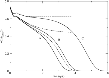
Figure 1: The $\phi(t)$ calculated from the unified theory, and the results of the idealized MCT are plotted for three temperatures. The solid lines A, B, C correspond to the full $\phi(t)$ for $\epsilon=-0.1$, $\epsilon=0$ and $\epsilon=0.5$, respectively. The dashed lines are the idealized MCT results. In this plot $\lambda=0.568$ which means that the MCT dynamics without hopping above $T_{c}$ is stretched with stretching parameter $\beta_{MCT}=0.8$. The activated dynamics is calculated with barrier height distribution such that $\beta^{static}_{hop}=0.5$.

In figure 1 we plot the results of the unified theory and also that of the idealized MCT ($F_{12}$ model). The plots are given for $\epsilon=-.1$, $\epsilon=0$ and $\epsilon=0.5$ which correspond to temperatures above, at and below $T_{c}$ respectively. The calculations are done at $\lambda=0.568$ which for idealized MCT above $T_{c}$ (for $\epsilon<0$ ) predicts a stretched relaxation with the MCT stretching parameter, $\beta_{MCT}=0.8$. For the activated dynamics we have considered Gaussian distribution of barriers that would predict the stretching parameter for the hopping dynamics, $\beta^{static}_{hop}=0.5$. As expected, hopping does not have much effect above $T_{c}$ but below $T_{c}$ the unified theory continues to show structural relaxation where the idealized MCT would have predicted strict localization transition. The longtime dynamics is stretched at all the temperatures. But as will be discussed later the stretching parameter for the total dynamics is different from $\beta_{MCT}$ and $\beta^{static}_{hop}$. Its value depends on the interaction between the hopping and the MCT dynamics and changes with temperature.

III The effect of hopping on the MCT dynamics above, at and below $T_{c}$ :Analytical results

In the earlier article we showed numerically that hopping has very little effect on the MCT dynamics above $T_{c}$ and has a nonlinear effect on the MCT relaxation timescale at $T_{c}$. In this article we analytically investigate the effect of hopping on the MCT dynamics above, at and below $T_{c}$. For this study we first examine the one parameter MCT dynamics, i.e. we consider $\lambda_{1}=0$. This is a special case of the two parameter model. The MCT transition takes place at $\lambda_{2}=4$ for $\lambda_{1}=0$. Initially we also take the barrier height distribution to be a delta function corresponding to a single hopping barrier. With these simplifications we use eqs.1-5 for the following analysis of the effect of hopping on the MCT timescale.

When $\lambda_{1}=0$, Eq.II can be rewritten as,

$$\frac{\Omega^{2}_{o}\phi_{MCT}(z)}{1+z\phi_{MCT}(z)}=z+i\gamma+LT\lambda_{2}\Omega^{2}_{o}[\phi^{2}(t)](z)$$ (6)

where LT stands for Laplace transform. Since we are interested in the $\alpha$ relaxation timescale we will take the longtime limit of the above equation. In the longtime limit where $z\rightarrow 0$, eq.6 reduces to,

$$\frac{\Omega^{2}_{o}\phi_{MCT}(z)}{1+z\phi_{MCT}(z)}=i\gamma+LT\lambda_{2}\Omega^{2}_{o}[\phi^{2}(t)](z)$$ (7)

In the above equation the second term on the right hand side is the self coupling term which makes dominant contribution at high density. But at low liquid density the self coupling term can be neglected and the solution of eq.7 is given by,

$$\phi_{MCT}(t)=e^{-K_{o}t}$$ (8)

where $K_{o}=\frac{\Omega^{2}_{o}}{\gamma}$ is the inverse timescale of longtime decay in the normal liquid regime.

Eq.7 in the time plane can be written as,

$${\bf\phi}_{MCT}(t)=\frac{1}{K_{o}}\dot{\bf\phi}_{MCT}(t)+\lambda_{2}\int_{0}^{t}\>dt^{\prime}{\bf\phi}^{2}(t^{\prime})\dot{\bf\phi}_{MCT}(t-t^{\prime})$$ (9)

From the earlier analysis sbp ; leu we know that the solution of eq.9 is exponential in the longtime. So we simplify $\phi_{MCT}(t)$ using its longtime form, $\phi_{MCT}(t)=ae^{-K_{MCT}t}$, where $a$ is the prefactor. Presently we also take the hopping part of the intermediate scattering function to be an exponential, $\phi_{hop}(t)=e^{-K_{hop}t}$. Using these expressions for $\phi_{MCT}$ and $\phi_{hop}$ in eq.9 we get an expression for $K_{MCT}$ in terms of $K_{hop},K_{o},\lambda_{2}$ and $a$.

$$K_{MCT}=\frac{1}{2} \Bigl{[} -(2K_{hop}-(1-a^{2}\lambda_{2})K_{o})$$

$$+ \sqrt{(2K_{hop}-(1-a^{2}\lambda_{2})K_{o})^{2}+8K_{hop}K_{o}}\Bigr{]}$$

In the absence of hopping the above expression reduces to,

$$K_{MCT}=(1-a^{2}\lambda_{2})K_{o}$$ (11)

Thus we see that the self coupling term leads to an increases in the timescale of relaxation when compared with the bare relaxation timescale $K^{-1}_{o}$. Eq.11 further predicts that $K_{MCT}$ goes to zero or the relaxation time approaches infinity as $a^{2}\lambda_{2}$ approaches one. Thus the analysis shows that in the absence of hopping strict localization takes place at $a^{2}\lambda_{2}=1$. From previous studies we know at $T_{c}$, $a=1/2$ and $\lambda_{2}=4$ sbp ; leu ; beng , thus at $T=T_{c}$, $a^{2}\lambda_{2}$ indeed becomes unity.

We will now analyze $K_{MCT}$ in the presence of hopping in three different regions, above $T_{c}$, at and around $T_{c}$ and below $T_{c}$.

III.1 Above $T_{c}$

Above the mode coupling transition temperature $T_{c}$, it was shown by explicit calculation that the timescale of hopping dynamics is so much longer than direct relaxation in the system that it can be neglected sbp . The expression of $K_{MCT}$ then reduces to,

$$K_{MCT}\simeq(1-a^{2}\lambda_{2})K_{o}$$ (12)

Thus in accord with our earlier numerical calculation sbp above the mode coupling transition temperature the hopping does not have significant effect on the $\alpha$ relaxation timescale.

III.2 At and around $T_{c}$

From the earlier studies we know that at the transition temperature, $a^{2}\lambda_{2}=1$ sbp ; leu . Thus eq.III reduces exactly to,

$$K_{MCT}=-K_{hop}+\sqrt{K^{2}_{hop}+2K_{hop}K_{o}}$$ (13)

In the above expression if we take some reasonable value for $K_{o}$ and $K_{hop}$, we find that,

$$K_{MCT}\simeq\sqrt{2K_{hop}K_{o}}$$ (14)

Thus we find that $K_{MCT}$ has a nonlinear dependence on $K_{hop}$ which is also in accord with our earlier numerical calculations sbp . The coupling of the hopping dynamics with the short time part of the MCT dynamics (liquid like dynamics) leads to this nonlinear dependence. Thus we find that coupling between the short time part of the MCT dynamics and hoppings leads to an MCT part of the structural relaxation timescale which is much faster than the hopping timescale. This is a critical effect and is found at and near $T_{c}$. This result corroborates our earlier findings that a single hopping event leads to many continuous diffusion events which are the primary means of structural relaxation in this region. In the next subsection we will find that this scenario changes as we go lower and lower in temperature.

III.3 Below $T_{c}$

Much below the transition temperature, $a^{2}\lambda_{2}>>1$. Eq.III can be rewritten as,

$$K_{MCT}=\frac{1}{2} \Bigl{[} ((a^{2}\lambda_{2}-1)K_{o}+2K_{hop})$$

$$\times{\Bigl{\{}}-1+\sqrt{1+\frac{8K_{hop}K_{o}}{((a^{2}\lambda_{2}-1)K_{o}+2K_{hop})^{2}}}{\Bigr{\}}}\Bigr{]}$$

Since at low temperatures $((a^{2}\lambda_{2}-1)K_{o}+2K_{hop})^{2}>>8K_{hop}K_{o}$ thus we can write,

$$K_{MCT}=\frac{2K_{hop}K_{o}}{((a^{2}\lambda_{2}-1)K_{o}+2K_{hop})}$$ (16)

Now if we further take into consideration that $(a^{2}\lambda_{2}-1)K_{o}>>2K_{hop}$ then the above equation reduces to,

$$K_{MCT}\simeq\frac{2K_{hop}}{(a^{2}\lambda_{2}-1)}$$ (17)

Thus much below the transition temperature the timescale of the MCT dynamics and also the total dynamics becomes slaved to the hopping timescale. Analyzing eq.17, an important observation can be made about the relaxation timescale. It is known that as we lower the temperature both $\lambda_{2}$ and $a$ increases. Thus the denominator in eq.17 will increase as we lower the temperature. From the analysis in the earlier subsection we know that initially to start with, below $T_{c}$ $K_{MCT}>>K_{hop}$, then as we keep lowering the temperature then depending on the temperature dependence of $\lambda_{2}$ and $a$ ,$K_{MCT}\simeq K_{hop}$. But as we further lower the temperature then slowly $K_{MCT}<<K_{hop}$. Thus in this regime although there will be hopping induced continuous diffusion but the primary mode of the structural relaxation becomes direct activated hopping itself.

IV Interplay between hopping and MCT dynamics at and below $T=T_{c}$ : Numerical results

Continuing from our analysis where both MCT and hopping dynamics are assumed to be exponential, here we will present some numerical results for the general case where both hopping and MCT dynamics can be stretched. For these general cases we will try to understand the effect of hopping on the MCT dynamics.

For the calculation we need to solve eq.II numerically. It is well known that due to the self consistent nature of the equation, its numerical solution becomes a nearly Herculean task around the mode coupling transition temperature. In the presence of hopping due to the disparate timescales present in the system and the convolution in eq.II which involves all these timescales, the time of calculation increases many fold. However the scheme proposed by Fuchs et al hofac allows the calculation to be done much faster. Both $\phi(t)$ and $\phi_{MCT}(t)$ vary more slowly for longer times than they do at short times. The essential idea involved in the scheme is to separate the slow and the fast variables and treat them differently in the convolution. The short time part of $\phi(t)$ and $\phi_{MCT}(t)$ are calculated exactly with very small stepsize and they are then used as input to carryout the calculation for the long time part of the same. We have exactly followed the scheme presented in reference hofac except for a minor modification (one extra term) in eq.29 of reference hofac when the integration timestep is an odd number. In our calculations the total timestep N=1000.

For this study we have picked three points on the $\lambda_{1}$, $\lambda_{2}$ plane. In all the cases to understand the temperature effect the values of $\lambda_{1}$, $\lambda_{2}$ were varied according to the expressions given bellow,

$$\lambda_{1}=\frac{(2\lambda-1)}{\lambda^{2}}+\epsilon\frac{\lambda}{(1+(1-\lambda)^{2})}$$ (18)

$$\lambda_{2}=\frac{1}{\lambda^{2}}+\epsilon\frac{\lambda(1-\lambda)}{(1+(1-\lambda)^{2})}$$ (19)

where the value of $\lambda$ determines the value of $\lambda_{1}$ and $\lambda_{2}$ at $T=T_{c}$. $\epsilon$ is a measure of the distance from the MCT transition temperature. As in our earlier model calculation, sbp the values of $\Omega^{\star}_{o}$ and $\gamma^{\star}$ are kept unity and the scaling time as 1ps. In the numerical calculations, to understand the temperature effect although we have changed the values of $\lambda_{1}$ and $\lambda_{2}$ but we have kept all the other parameters constant including the hopping barriers. For the calculation of the hopping part we have used eq.5 with a Gaussian distribution of barriers. According to the RFOT theory, the mean barrier height and thus the hopping timescale should change with temperature xiawoly ; lubwoly . In its simplest form without taking barrier softening into consideration the mean barrier height can be written as, $\Delta F/k_{B}T=32k_{B}/s_{c}=\frac{32k_{B}}{\Delta c_{p}}\frac{T_{K}}{(T-T_{K})}$, where $s_{c}$ is the configurational entropy, $\Delta c_{p}$ is the jump in the specific heat and $T_{K}$ is the Kauzmann temperature xiawoly ; lubwoly . However in this present calculation to clearly assign any change in dynamics due to the change in $\lambda_{1}$ and $\lambda_{2}$ value we have kept the mean of the distribution fixed at about 8.8 $k_{B}T$. As mentioned earlier the stretching in the hopping dynamics is determined by the width of the Gaussian distribution of the barriers. The broader the distribution the more stretched is the dynamics. We have varied the width of the distribution such that the $\beta^{static}_{hop}$ varies from 0.2 to 0.8. Along with the $\beta^{static}_{hop}$ value the timescale of hopping also changes, which has been taken into account in our calculation.

For all the cases the $\beta_{total}$ values are plotted against $\beta^{static}_{hop}$ for different $\epsilon$ values, where $\beta_{total}$ is the stretching parameter for $\phi(t)$ and $\beta^{static}_{hop}$ is the same for $\phi_{hop}(t)$.

IV.1 Case 1: $\lambda=0.5$

In the first case we consider an example when $\lambda=0.5$. This value of $\lambda$ implies that at $T=T_{c}$, $\lambda_{1}=0$ and $\lambda_{2}=4$ and the MCT dynamics just above $T_{c}$ is exponential. For this case we vary $\epsilon$ from $0-1$. In figure 2, the $\beta_{total}$ values are plotted against $\beta^{static}_{hop}$ for the three $\epsilon$ values. As expected for $\epsilon=0$ the $\beta_{total}\simeq 1$. This is because although without hopping structural relaxation is arrested but once hopping is present the relaxation is dominated by the MCT dynamics. As we increase the epsilon value we find that the effect of hopping is stronger and the dynamics gets stretched. But we also notice that for very low $\beta^{static}_{hop}$ value the dynamics is less stretched than the static barrier distribution would indicate. This is because lower $\beta^{static}_{hop}$ value implies a broader barrier height distribution which means we populate both lower and higher barrier heights. The small barrier hoppings actually couple to the liquid like part of the MCT dynamics (whose timescale is given by $K_{o}^{-1}$) and the relaxation is faster and dominated by this liquid like MCT dynamics which has a much shorter timescale. As we increase the $\epsilon$ value MCT gets more slaved to hopping and thus the time scale of relaxation increases and the liquid like MCT dynamics becomes less important. If we further lower the temperature (or increase the $\epsilon$ value) we would find that even for small $\beta^{static}_{hop}$ values the total dynamics is determined primarily by hopping.

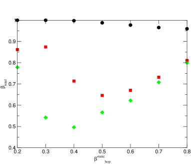
Figure 2: The stretching parameter for the total structural relaxation, $\phi(t)$, $\beta_{total}$ is plotted against the same for $\phi_{hop}(t)$, $\beta^{static}_{hop}$ for three different $\epsilon$ values. The solid circle is for $\epsilon=0$, the solid square is for $\epsilon=0.5$ and the solid diamond is for $\epsilon=1$. In this plot the $\lambda=0.5$ which means that the MCT dynamics without hopping above $T_{c}$ is exponential.

The interplay of hopping with MCT nonlinearities can be thought of as a quantitative formulation of ”facilitation effects” xiawoly . As Xia and Wolynes pointed out hopping events interact if they occur near each other. This is accounted for by the MCT nonlinearity. In the Xia-Wolynes treatment the corresponding effect led to the cutoff of the relaxation time distribution, on the slow side, owing to the renewal of a mosaic cell’s environment through hops. This resulted in an increased $\beta$ from that obtained from the static Gaussian model, as occurs here too xiawoly .

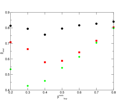
Figure 3: The stretching parameter for the total structural relaxation, $\phi(t)$, $\beta_{total}$ is plotted against the same for $\phi_{hop}(t)$, $\beta^{static}_{hop}$ for three different $\epsilon$ values. The solid circle is for $\epsilon=0$, the solid square is for $\epsilon=0.5$ and the solid diamond is for $\epsilon=1$. In this plot the $\lambda=0.568$ which means that the MCT dynamics without hopping above $T_{c}$ is stretched with stretching parameter, $\beta_{MCT}=0.8$.

IV.2 Case 2: $\lambda=0.568$

In this case we consider that $\lambda=0.568$. This value of $\lambda$ implies that at $T=T_{c}$, $\lambda_{1}=.4215$ and $\lambda_{2}=3.09958$ and the MCT dynamics, (without hopping) just above $T_{c}$, would already be stretched with $\beta_{MCT}=0.8$. For this case we vary $\epsilon$ from $0-1$. In figure 3, the $\beta_{total}$ values are plotted against $\beta^{static}_{hop}$ for the three $\epsilon$ values. The results are similar to those obtained for the first case. For $\epsilon=0$ the $\beta_{total}\simeq 0.8$ which implies that the total dynamics is still determined primarily by the MCT dynamics. We also find that for high $\beta^{static}_{hop}$ values, as $\epsilon$ increases, the dynamics gets more and more dominated by the hopping dynamics. Nevertheless, for small $\beta^{static}_{hop}$ the scenario is a little different. For smaller $\epsilon$ values the low barrier hoppings couple to the liquid like part of the MCT dynamics and the dynamics is less stretched and also much faster. However, as we increase $\epsilon$, MCT dynamics gets more and more slaved to hopping dynamics and the MCT relaxation timescale becomes proportional to the hopping relaxation timescale (similar to that shown in Eq.17). Thus the effect of the coupling of low barrier hoppings with the liquid like part of the MCT dynamics, on the total MCT dynamics, reduces. If we further lower the temperature then we would find that even for $\beta^{static}_{hop}=0.2$ the total dynamics follows the hopping dynamics.

The results in case 1 and case 2 look quite similar but more detailed observation reveals that the value of $\beta^{static}_{hop}$, where $\beta_{total}$ begins to increase, is smaller for case 2 (where MCT dynamics itself is more stretched) than it is in case 1. As discussed earlier, the reason $\beta_{total}$ increases for small $\beta^{static}_{hop}$ is that the small barrier hopping gets coupled to the liquid like part of the MCT dynamics allowing the total structure to relax. Now in case 2, the MCT dynamics is itself stretched thus the effect of the small barrier hopping on the MCT dynamics will be much less effective when compared to case 1. This trend becomes clearer when we study the next case where the MCT dynamics is much more stretched.

IV.3 Case 3: $\lambda=0.75$

In this case we consider that $\lambda=0.75$. This value of $\lambda$ implies that at $T=T_{c}$, $\lambda_{1}=.889$ and $\lambda_{2}=1.778$ and the MCT dynamics (without hopping) just above $T_{c}$ would already be stretched with $\beta_{MCT}=0.5$. For this case we vary $\epsilon$ from $0-1$. In figure 4, the $\beta_{total}$ values are plotted against $\beta^{static}_{hop}$ for the three $\epsilon$ values. The results are similar to that obtained for case 1 and case 2 for $\epsilon=0$. But for higher $\epsilon$ values unlike in case 1 and 2, $\beta_{total}$ continuously decreases with $\beta^{static}_{hop}$. This is because as discussed before, since MCT dynamics is already stretched, the structural relaxation due to low barrier hopping is less effective. Also note that the $\beta_{total}$ decreases with $\beta^{static}_{hop}$ value but it is neither equal to $\beta^{static}_{hop}$, nor equal to the pre-transition $\beta_{MCT}$ value. At these temperatures although MCT dynamics is slaved to hopping but both the channels of relaxation are almost equally effective. If we compare the $\beta_{total}$ values for $\epsilon=$ 0.5 and 1, we will find that in most of the cases $\beta_{total}$ for $\epsilon=1$ has a lower value. This is because at lower temperatures MCT dynamics becomes a less effective relaxation channel. At further lower temperatures (higher $\epsilon$ values) $\beta_{total}$ will follow $\beta^{static}_{hop}$ more closely.

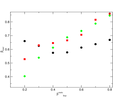
Figure 4: The stretching parameter for the total structural relaxation, $\phi(t)$, $\beta_{total}$ is plotted against the same for $\phi_{hop}(t)$, $\beta^{static}_{hop}$ for three different $\epsilon$ values. The solid circle is for $\epsilon=0$, the solid square is for $\epsilon=0.5$ and the solid diamond is for $\epsilon=1$. In this plot the $\lambda=0.75$ which means that the MCT dynamics without hopping above $T_{c}$ is stretched with stretching parameter, $\beta_{MCT}=0.5$.

V Concluding Remarks

MCT and the RFOT theory provide a unified theory of relaxation over the whole temperature plane sbp . Even without dynamical heterogeneity the theory successfully predicts the decay of the structural relaxation below mode coupling transition temperature, $T_{c}$, confirming there is no strict localization transition at $T_{c}$. Without dynamical heterogeneity of the instantons the coupled theory lead to an exponential $\alpha$ relaxation, but in the laboratory the $\alpha$ relaxation is generally stretched. In the present article we examined both a two parameter MCT model gotze and more realistically one that also included a barrier height distribution that gives rise to stretching in the hopping dynamics by itself xiawoly .

The study has been carried out for different stretching parameters of the MCT dynamics, that is by changing $\lambda$ values in the $F_{12}$ model and also for different stretching parameters of the hopping dynamics obtained by changing the width of the distribution of barrier heights.

To summarize, the main conclusions of the present work is that the continuous dynamics, described here within the $F_{12}-$MCT formalism , and the activated hopping dynamics, described here using RFOT theory, interact in a non-linear fashion to give rise to dynamical features which are distinct from both. MCT by itself of course cannot describe dynamics below its critical temperature. We find that hopping facilitates the continuous dynamics channel and in the process the effects of hopping on the relaxation decreases. Thus, one finds the stretching parameter arising solely from distribution of hopping barrier energies in RFOT is increased by the mode coupling terms. It is also found that when MCT dynamics is less stretched then the effect of hopping on the MCT dynamics is less pronounced and the hopping dominated regime moves to a lower temperature. On the other hand, for more stretched MCT dynamics, due to the larger overlap of MCT and hopping timescales, hopping begins to dominate at a higher temperature.

We have already mentioned the need for using a more complex hopping kernel than that given by Eqs.3-5. In particular, one needs to include the effects of mode coupling softening on the barrier height distribution. This is a feed-back effect of unleashing the mode coupling relaxation channels due to hopping, on the barrier height distribution itself. This non-linear feed-back is expected to shift the distribution to lower barrier heights and in turn accelerate mode coupling relaxation which can further enhance hopping. The whole system of equations needs to be solved self-consistently. To achieve this, we need to understand more quantitatively the effects of softening on the barrier height distribution.

ACKNOWLEDGEMENT

This work was supported in parts from NSF (USA) and DST (India).

References

- (1) S. M. Bhattacharyya, B. Bagchi, P. G. Wolynes, Phys. Rev. E 72 031509 (2005).
- (2) W. Gotze and L. Sjogren, Z. Phys. B- Cond. Mat., 65, 415 (1987);W. Gotze and L. Sjogren, J. Phys. C:Solid State Phys. 21, 3407 (1988).
- (3) S. P. Das and G. F. Mazenko, Phys. Rev. A, 34, 2265 (1986).
- (4) T.R. Kirkpatrick and P.G. Wolynes, Phys. Rev. E 35, 3072 (1987).
- (5) J. P. Bouchaud and G. Biroli, J. Chem. Phys. 121, 7347 (2004).
- (6) S. Bhattacharyya, A. Mukherjee, and B. Bagchi, J. Chem. Phys.117, 2741(2002); S. Bhattacharyya and B. Bagchi, Phys. Rev. Lett. 89, 025504-1(2002); A. Mukherjee, S. Bhattacharyya and B. Bagchi, J. Chem. Phys. 116, 4577 (2002);
- (7) X. Xia and P. G. Wolynes, Phys. Rev. Lett. 86, 5526 (2001);Proc. Natl. Acad. Sci. U. S. A. 97, 2990 (2000).
- (8) V. Lubchenko and P. G. Wolynes, J. Chem. Phys. 119, 9088 (2003);
- (9) E. Leutheusser, Phys. Rev. A 29, 2765 (1984).
- (10) U. Bengtzelius, W. Gotze, and A. Sjolander, J. Phy. C 17, 5915 (1984).
- (11) M. Fuchs, W. Gotze, I. Hofacker and A.Latz, J. Phys: Condensed Matter 3, 5047 (1991).