Wave Propagation in the Cantor-Set Media:
Chaos from Fractal

Abstract

Propagation of waves in the Cantor-set media is investigated by a renormalization-group type method. We find fixed points for complete reflection, $T^{*}=0$, and for complete transmission, $T^{*}=1$. In addition, the wave numbers for which transmission coefficients show chaotic behaviors are reported. The results obtained are for optical waves, and they can be tested in optical experiments. Our method could be applied to any wave propagation through the Cantor set.

Localization of the electronic states due to disorder is an active field in condensed matter physics. It has been recognized that localization occurs not only in disordered systems but also in quasiperiodic systems in one dimension MK83 ; KO84 ; MK86 . While the localization of states was originally regarded as an electronic problem, it was later recognized that the phenomenon is essentially a consequence of the wave nature of electronic states. Therefore, such localization can be expected for any wave phenomenon. An optical experiment with the Fibonacci multilayer was proposedmk87 , and the corresponding experiments using dielectric multilayer stacks of SiO₂ and TiO₂ thin films were reportedwg94 ; th94 . The transmission coefficients and scaling properties well agree with the theorymk87 , and can be considered as an experimental evidence for localization of electromagnetic waves. Recently, an experiment for propagation of electromagnetic waves in a three-dimensional fractal cavity was reportedmw04 , where a confinement of electromagnetic waves in the fractal structure was observed.

Propagation of light in the Cantor media was numerically studied by Konotop et al.ko90 and Sun and Jaggard xs91 , later by Bertolotti et al. with transfer matricesmp94 ; mb96 , and recently by Yamanaka and Kohmotonh05 and Hatanonh06 again with transfer matrices. Comparison of the experimental results and numerical results was performed by Lavrinenko et al.av02 .

We study wave propagation in the Cantor-set media by a renomalization-group type methodkadanoff . For specific values of the wave numbers, transmission coefficients show chaotic behaviors governed by the logistic map. This exotic behavior could be observed in an optical experiment. In this system, the one-dimentional theory is strictly valid. In addition, it is feasible to construct the system accurately, and the parameters can be precisely controlled and measured.

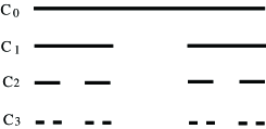
Figure 1: The initial state $j=0$ and the first three generations in the construction of the Cantor set.

The procedure of constructing the Cantor set begins with a line segment with unit length. We regard this as substrate A. The line segment is divided into three parts. The left and the right segments are substrate A, each of which has length ${1}/{3}$. The middle part, which has length ${1}/{3}$, is removed. We regard the removed part as substrate B. The procedure is repeated for each of line segments A. We call $j$-th generation of the Cantor sequence as C_j. For C_j we have a set of $2^{j}$ line segments of substrate A, each of which has length ${1}/{3^{j}}$. The Cantor set is obtained if this procedure is repeated infinite times. It is self-similar and has the fractal dimension $\log{2}/\log{3}$. Constructions of first few generations are shown in Fig.1. In the following, we suppose that the indices of refraction of A and B are $n_{\rm A}$ and $n_{\rm B}$, and the magnetic permeabilities of A and B are $\mu_{\rm A}$ and $\mu_{\rm B}$, respectively.

We consider wave propagation through C_j. See Fig.2. For simplicity, suppose that the incident light is normal and the polarization is perpendicular to the plane of the light path. Here $E_{\rm L}^{(1)}$ represents the incident light, and $E_{\rm L}^{(2)}$ and $E_{\rm R}^{(1)}$ represent reflected and transmitting light, respectively. We also consider light coming from right $E_{\rm R}^{(2)}$.

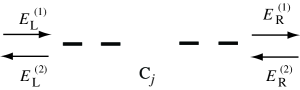
Figure 2: Electromagnetic wave propagation through the Cantor sequence C_j.

By setting

$$E_{+}=E^{(1)}+E^{(2)},\quad E_{-}=(E^{(1)}-E^{(2)})/i,$$ (1)

the wave propagation is given bymk87 ; nh05

$$\left(\begin{array}[]{c}E_{+}\\ E_{-}\end{array}\right)_{\rm R}={\cal M}_{j}(k)\left(\begin{array}[]{c}E_{+}\\ E_{-}\end{array}\right)_{\rm L},$$ (6)

where ${\cal M}_{j}$ satisfies

$${\cal M}_{j+1}(k)={\cal M}_{j}(\frac{k}{3}){\cal T}(\frac{n_{\rm B}k}{3}){\cal M}_{j}(\frac{k}{3}),$$ (7)

with the initial condition

$${\cal M}_{0}(k)={\cal T}_{\rm BA}{\cal T}(n_{\rm A}k){\cal T}_{\rm AB}.$$ (8)

Here $k$ is a wave number in vacuum, and the matrices ${\cal T}_{\rm AB}$ and ${\cal T}_{\rm BA}$ represent light propagation across interfaces $A\leftarrow B$ and $B\leftarrow A$ respectively,

$${\cal T}_{\rm AB}={\cal T}_{\rm BA}^{-1}=\left(\begin{array}[]{cc}1&0\\ 0&1/n\end{array}\right),\quad n=\frac{n_{\rm A}}{n_{\rm B}}\times\frac{\mu_{\rm B}}{\mu_{\rm A}}.$$ (11)

The matrix ${\cal T}(\delta)$ represents light propagation within a layer,

$${\cal T}(\delta)=\left(\begin{array}[]{cc}\cos\delta&-\sin\delta\\ \sin\delta&\cos\delta\end{array}\right).$$ (14)

For a layer of type A and B with thicknesses $d$, the phase $\delta$ is given by $\delta=n_{\rm A}kd$ and $\delta=n_{\rm B}kd$, respectively. Equation (7) can be regarded as a renormalization-group transformation. One can easily show that

$$\det{\cal M}_{j}=1.$$ (15)

By putting $E_{\rm R}^{(2)}=0$, the transmission coefficient $T_{j}$ of ${\rm C}_{j}$ is given by

$$T_{j}=\frac{4}{|{\cal M}_{j}|^{2}+2},$$ (16)

where $|{\cal M}_{j}|^{2}$ is the sum of the squares of each matrix element of ${\cal M}_{j}$.

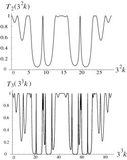
Figure 3: Transmission coefficient $T_{j}$ as a function of the wave number $k$ for C₂ (top) and C₃ (bottom). ($n_{\rm A}=2$, $n_{\rm B}=1$ and $n=2$.) The range of the wave number $k$ for C_j is $0\leq k\leq 3^{j}\pi$. Note that the horizontal axes are rescaled.

An example of transmission coefficients as a function of wave numbers is shown in Fig.3 for C₂ and C₃. They show a scaling behavior when one multiplies wave numbers by three each time one increases a generation. Thus we study wave propagation of wave numbers $3^{j}k$ of C_j.

In C_j, all A’s have the same length $1/3^{j}$, thus the propagation in A’s are given by the unique transfer matrix ${\cal T}(n_{\rm A}k)$. On the other hand, B’s have lengths $1/3^{j},1/3^{j-1},\cdots$ and $1/3$, thus in general they give $j$ different transfer matrices, which are given by ${\cal T}(n_{\rm B}k),{\cal T}(3n_{\rm B}k),\cdots$, and ${\cal T}(3^{j-1}n_{\rm B}k)$. However, if $k$ is given by

$$n_{\rm B}k=\frac{m\pi}{3^{q}},$$ (17)

with integers $m$ and $q$, ${\cal T}(\delta)$’s in large B’s are equal to ${\cal T}(m\pi)$. Now the map (7) for $j\geq q$ is written as

$${\cal N}_{j+1}={\cal N}_{j}^{2},$$ (18)

where

$${\cal N}_{j}={\cal T}(m\pi){\cal M}_{j}.$$ (19)

From (15), ${\cal N}_{j}$ satisfies

$${\rm det}{\cal N}_{j}=1.$$ (20)

To solve (18), we rewrite ${\cal N}_{j}$ in terms of the Pauli matrices $\sigma_{i}$ $(i=1.2.3)$,

$${\cal N}_{j}= x_{j}{\bm{1}}+{\bm{a}}_{j}\cdot{\bm{\sigma}},\quad{\bm{a}}_{j}=(a_{j}^{(1)},ia_{j}^{(2)},a_{j}^{(3)}),$$ (21)

where $x_{j}$ and $a_{j}^{(i)}$ $(i=1,2,3)$ are real. Comparing the coefficients of ${\bm{1}}$ and ${\bm{\sigma}}$ in both side of (18), we have

$$x_{j+1}=x_{j}^{2}+{\bm{a}}_{j}^{2},$$ (22)

and

$${\bm{a}}_{j+1}=2x_{j}{\bm{a}}_{j}.$$ (23)

In addition, (20) leads to

$$x_{j}^{2}-{\bm{a}}_{j}^{2}=1.$$ (24)

From (22) and (24), we have the map for $x_{j}=\frac{1}{2}{\rm Tr}{\cal N}_{j}$

$$x_{j+1}=2x_{j}^{2}-1,\quad(j\geq q).$$ (25)

This is the logistic map which maps the interval $[-1,1]$ onto itself and others to $+\infty$. The bounded $x_{j}$’s are given by

$$x_{j}=\cos[2^{j-q}(\cos^{-1}{x_{q}})],$$ (26)

and have chaotic behaviors with the Lyapunov exponent $\ln 2$.

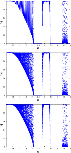
Figure 4: Transmission coefficient $T_{j}$ as a function of $n$ for $n_{\rm B}k=\pi/3$. Iteration number is $j=5$ (top), $j=10$ (center), and $j=100$ (bottom).

From (23), we also find the following constants of motion $\lambda$ and $\eta$

$$\frac{a_{j}^{(3)}}{a_{j}^{(2)}}=\lambda,\quad\frac{a_{j}^{(1)}}{a_{j}^{(2)}}=\eta\quad(j\geq q).$$ (27)

In terms of them, the transmission coefficient (16) is given by

$$T_{j}=\frac{1-(\lambda^{2}+\eta^{2})}{1-(\lambda^{2}+\eta^{2})x_{j}^{2}}.$$ (28)

If the constants of motion $\lambda$ and $\eta$ satisfy $0\leq\lambda^{2}+\eta^{2}\leq 1$, we have $|x_{j}|\leq 1$. Then, the complete transmission $T_{j}=1$ is achieved when $x_{j}=\pm 1$, and we have the minimal transmission

$$T_{\rm min}=1-(\lambda^{2}+\eta^{2}),$$ (29)

when $x_{j}=0$. On the other hand, if ${\lambda}^{2}+{\eta}^{2}>1$ we have $|x_{j}|>1$. Then $x_{j}$ escapes to infinity and the transmission coefficient flows into the fixed point for complete reflection $T^{*}=0$, as seen from (28). We show the transmission coefficient $T_{j}$ as a function of $n$ for $n_{\rm B}k=\pi/3$ in Fig.4. Since the complete reflections and the complete transmissions are nearby in $n$, the Cantor media could be used as a fast swiching devices.

We note that similar chaotic behaviors also appear for the initial wave numbers

$$n_{\rm B}k=\frac{m+1/2}{3^{q}}\pi,$$ (30)

with integers $m$ and $q$. The matrix ${\cal T}(\delta)$ in large B’s is now ${\cal T}((m+1/2)\pi)$, and the map for ${\cal N}_{j}$ is ${\cal N}_{j+1}=-{\cal N}_{j}^{2}$. The trace of ${\cal N}_{j}$ follows the logistic map, again.

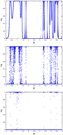
Figure 5: Transmission coefficient $T_{j}$ as a function of $n$ for $n_{\rm B}k=\pi/4$. Iteration number is $j=5$ (top), $j=10$ (center), and $j=100$ (bottom).

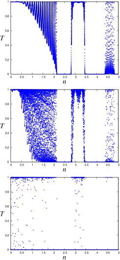
Figure 6: Transmission coefficient $T_{j}$ as a function of $n$ for $n_{\rm B}k=\pi/3+0.0001$. Iteration number is $j=5$ (top), $j=10$ (center), and $j=100$ (bottom).

For initial wave numbers other than (17) or (30), our numerical calculations suggest that light reflects completely or transmits completely by the Cantor-set media. An example of our numerical results are shown in Fig.5. The transmission coefficients tend to flow into the fixed point $T^{*}=0$ or $T^{*}=1$ as the generation increases.

When initial wave numbers are near a value (17) or (30), the transmission coefficients show chaotic behaviors in first few generations. For example, the transmission coefficients $T_{j}$ for $n_{\rm B}k=\pi/3+0.0001$ are shown in Fig.6. In the fifth generation ($j=5$), the transmission coefficients show chaotic behaviors indistinguishable from the case for $n_{\rm B}k=\pi/3$ (Fig.4). However, in the tenth generation ($j=10$), the transmission coefficients show different behaviors from the case for $n_{\rm B}k=\pi/3$, and in the hundredth generation ($j=100$), they tend to flow into the fixed point $T^{*}=0$ or $T^{*}=1$. Our numerical results again suggest that light reflects completely or transmits completely by the Cantor-set media. This behavior should be observed experimentally.

We can also study wave propagation for other types of Cantor-set media by using similar recursion relations as (7). Chaotic behaviors governed by the logistic map occur in the Cantor-set media, if the length of each A becomes $1/\alpha$ each time one increases a generation, and $\alpha$ is an integer. Details will be given in a separated paper ESK .

We acknowledge useful discussions with M. Yamanaka.

References

- (1) M. Kohmoto, L.P. Kadanoff, and C. Tang, Phys. Rev. Lett. 50, 1870(1983).
- (2) M. Kohmoto and Y. Oono, Phys. Lett. 102A, 145(1984).
- (3) M. Kohmoto, B. Sutherland, and C. Tang, Phys. Rev. B. 35, 1020(1987).
- (4) M. Kohmoto, B. Sutherland, and K. Iguchi, Phys. Rev. Lett. 58, 2436(1987).
- (5) W. Gellermann, M. Kohmoto, B. Sutherland, and P.C. Taylor, Phys. Rev. Lett. 72, 633(1994).
- (6) T. Hattori, N. Tsurumachi, S. Kawato, and H. Nakatsuka, Phys. Rev. B.50, 4220(1994).
- (7) M. W. Takeda, S. Kirihara, Y. Miyamoto, K. Sakoda, and K. Honda, Phys. Rev. Lett. 92, 093902(2004).
- (8) V. V. Konotop, O. I. Yordanov, and I. V. Yurkevich, Europhys. Lett. 12, 481(1990).
- (9) X. Sun and D.L. Jaggard, J.Appl.Phys. 70, 2500(1991).
- (10) M. Bertolotti, P. Masciulli, and C. Sibilia, Opt. Lett. 19, 777(1994).
- (11) M. Bertolotti, P. Masciulli, C. Sibilia, F. Wijnands, and H. Hoekstra, J.Opt. Soc. Am.B 13, 628(1996).
- (12) M. Yamanaka and M. Kohmoto (unpublished) cond-mat/0410239.
- (13) N. Hatano, J. Phys. Soc. Jpn. 74, 3093(2005).
- (14) A.V. Lavrinenko, S.V.Zhukovsky, K.S. Sandomirski, and S.V. Gaponenko, Phys. Rev. E. 65, 036621(2002).
- (15) L.P. Kadanoff, Statistical Physics (World Scientific, 2000).
- (16) K. Esaki, M. Sato, and M. Kohmoto, in preparation.