Phase-dependent noise correlations in normal-superconducting structures

Abstract

We study nonequilibrium noise correlations in diffusive normal-superconducting structures in the presence of a supercurrent. We present a parametrization for the quasiclassical Green’s function in the first order of the counting field $\chi$. This we employ to obtain the voltage and phase dependence of cross and autocorrelations and to describe the role played by the setup geometry. We find that the low-voltage behavior of the effective charge $q_{\rm eff}$ describing shot noise is a result of a competition between anticorrelation of Andreev pairs due to proximity effect and the depression of the local density of states. Furthermore, we show that the noise correlations are independent of the sign of the supercurrent.6

The charge transmitted through a disordered conductor in unit time varies due to the quantum nature of the transport process. This variation is characterized by the current distribution, whose width at low temperatures is directly related to the shot noise.Ya. M. Blanter and M. Büttiker (2001) In metallic conductors, the corrections induced by the quantum coherence on the current and conductance distributions are small,K. A. Muttalib et al. (2003); Stenberg and Särkkä (2006) but in a metal in contact to a superconductor, more pronounced effects may be observed, e.g., in the out-of-equilibrium noise experiments.X. Jehl et al. (2000); Kozhevnikov et al. (2000); F. Lefloch et al. (2003); Reulet et al. (2003) In the context of a normal-superconducting (NS) two-terminal setup, the theoretical endeavours have recently covered, e.g., the voltage dependence of the shot noise Belzig and Nazarov (2001); Stenberg and Heikkilä (2002) and certain low-bias anomalies.Stenberg and Heikkilä (2002); Houzet and Pistolesi (2004) Multiterminal structures have been discussed in the incoherent regime,Nazarov and Bagrets (2002); Samuelsson and Büttiker (2002); W. Belzig and P. Samuelsson (2003); P. Virtanen and T. T. Heikkilä (2006) and in the presence of a supercurrent, in a short junction,Bezuglyi et al. (2004) and for specific values of a phase difference in a three-terminal setup. The latter was described by a method based on a direct discretization of the equations governing the full counting statistics [see Eq. (1)].Reulet et al. (2003)

In the presence of the superconducting proximity effect and at voltages of the order of $E_{T}/e$, the effective charge $q_{\rm eff}$ characterizing the magnitude of shot noise is lower than $2e$, the value corresponding to a Cooper pair.Belzig and Nazarov (2001); Stenberg and Heikkilä (2002); Reulet et al. (2003) Here $E_{T}=\hbar D/L^{2}$ is the Thouless energy, with $D$ the diffusion constant and $L$ the wire length. Applying a supercurrent in a three-terminal structure (Fig. 1) allows one to study the nature of this proximity-induced change in $q_{\rm eff}$. For example, with this approach, we directly show that the lowering of $q_{\rm eff}$ is due to a competition of anticorrelation effects induced by the superconducting proximity effect Reulet et al. (2003) and the depression of the local density of states.Zhou et al. (1998) In principle, the effect of an extra current in the system would be twofold: to tune the coherent effects and to induce its own correlations. Here we show that within our noninteracting model supercurrent does only the previous as all the correlations in the system are independent of the supercurrent sign.

The full counting statistics L. S. Levitov et al. (1996); Yu. V. Nazarov, Ann. Phys. (Berlin); W. Belzig in Quantum Noise in Mesoscopic Physics, edited by Yu. V. Nazarov (Kluwer, Dordrecht, 2003) has recently become the method of choice to calculate shot noise in diffusive mesoscopic conductors but, to our knowledge, the cross correlations in the presence of supercurrent have not been studied. The statistics is accessed by performing a counting rotation of the Green’s function $\check{g}_{0}$ in one of the terminals, using the counting field $\chi$.W. Belzig in Quantum Noise in Mesoscopic Physics, edited by Yu. V. Nazarov (Kluwer, Dordrecht, 2003) To access the noise correlations, one has to expand the resulting function $\check{g}(\chi)=\check{g}_{0}-i(\chi/2)\check{g}_{1}+\mathcal{O}(\chi^{2})$ in powers of the counting field and solve the problem in the first order in $\chi$. Within quasiclassical formalism, the spectral quantities related to $\check{g}_{0}$ may be represented by two parameters, $\theta$ and $\phi$ characterizing the magnitude and phase of the pair correlations. The distributions of the electrons and holes are treated by dividing the functions into even and odd components with respect to the Fermi surface, $f_{T}$ and $f_{L}$.W. Belzig et al. (1999) In the absence of supercurrent, a parametrization for $\check{g}_{1}$ has been given in Ref. Houzet and Pistolesi, 2004.

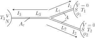
Figure 1: Setup schematic studied in this work.

Here we present a parametrization for $\check{g}_{1}$ applicable also for a finite supercurrent. Since the resulting essentially linear method is considerably faster than the previous “direct discretization” approach, we have been able to extensively study the roles played by the setup geometry, dissipative currents, coherence and phase gradients.

In our setup (Fig. 1), the two superconducting terminals $T_{1}$ and $T_{2}$ are connected by diffusive wires $1$ and $2$ and, at the central node, by a diffusive control wire $3$ to a normal reservoir, $T_{3}$. The phase difference $\Delta\phi=\phi_{2}-\phi_{1}$ between the superconductors may be generated by fabricating a superconducting loop and applying a magnetic flux through the loop or by an external driving of supercurrent. The lengths of the wires are denoted by $L_{1,2,3}$ and the currents into the terminals $I_{1,2,3}$. We designate the cross section of the control wire by $A_{c}$ and suppose that the other wires are equally wide, with cross section $A$. The electric potential is assumed to vanish in the superconductors. We assume good contacts at the interfaces and a vanishing temperature and consider voltages below the superconducting energy gap $V\ll\Delta/e$.

In the quasiclassical diffusive limit, the triangular matrix $\check{g}_{0}=\check{g}(\chi=0)$ in Nambu($\hat{\ }$)-Keldysh($\bar{\ }$) space may be expressed through $\hat{R}$, $\hat{A}$, and $\hat{K}$, which may be parametrized using $\hat{A}=-\hat{\tau}_{3}\hat{R}^{{\dagger}}\hat{\tau}_{3}$, $\hat{K}=\hat{R}\hat{h}-\hat{h}\hat{A}$, $\hat{h}=f_{L}+f_{T}\hat{\tau}_{3}$, $\hat{R}=\cosh(\theta)\hat{\tau}_{3}+\sinh(\theta)(\cos(\phi)i\hat{\tau}_{2}+\sin(\phi)i\hat{\tau}_{1})$.W. Belzig et al. (1999) Here $\theta$ characterizes the strength of the superconducting proximity effect, $\phi$ is the superconducting phase, and $\hat{\tau}_{i}$ are the Pauli matrices in Nambu space. The counting field $\chi$, which we introduce in the normal reservoir, appears as a gauge transformation of the Green’s function in the same terminal.W. Belzig in Quantum Noise in Mesoscopic Physics, edited by Yu. V. Nazarov (Kluwer, Dordrecht, 2003) At a vanishing temperature, it suffices to concentrate only on the energy regime $0<\varepsilon<eV$. In this case, without counting rotation, one has in the normal terminal $\check{g}_{N,0}=\check{g}_{N}(\chi=0)=\hat{\tau}_{3}\otimes\bar{\sigma}_{3}+\hat{\tau}_{0}\otimes(\bar{\sigma}_{1}+i\bar{\sigma}_{2})$, where $\bar{\sigma}_{i}$ are Pauli matrices in Keldysh space. In the superconducting terminals we have $\check{g}_{S}=(\cos(\phi)\hat{\tau}_{2}+\sin(\phi)\hat{\tau}_{1})\otimes\bar{\sigma}_{0}$. The generalized Green’s functions $\check{g}(\chi)$ obey the Usadel equation Usadel (1970) similar to that in the zeroth order in $\chi$

$$-\frac{\hbar D}{LG_{D}}\partial_{x}\check{J}(x)=-i\varepsilon\left[\check{\tau}_{3},\check{g}(x)\right],$$ (1)

with $\check{J}(x)=-LG_{D}\check{g}(x)\partial_{x}\check{g}(x)$, $\check{\tau}_{3}=\hat{\tau}_{3}\otimes\bar{\sigma}_{0}$. Here $G_{D}$ is the normal-state conductance of the wire with length $L$, $x$ is the coordinate along the wire, and $\varepsilon$ is the energy. The Green’s function satisfies the normalization condition $\check{g}^{2}(\chi)=\hat{\tau}_{0}\otimes\bar{\sigma}_{0}$. At the NS interfaces the Nazarov boundary conditions Nazarov (1999) for $\check{g}(\chi)$ hold.

We obtain the noise correlations from

$$S_{ij}\equiv\int_{-\infty}^{\infty}\mathrm{d}t\langle\{\delta I_{i}(t),\delta I_{j}(0)\}\rangle=-2ie\frac{\partial J_{i}(\chi)}{\partial\chi_{j}}|_{\chi=0}.$$ (2)

Here we have $\qquad J(\chi)=-1/(8e)\int d\varepsilon\mathrm{Tr}[\check{\tau}_{K}\check{J}(x)]$ and $\delta I_{i}=I_{i}-\bar{I}_{i}$ is the deviation of the current from its quantum mechanical expectation value. In this article we take $j=3$ and thus with $i=3$ we get the noise $S_{33}\equiv S$ and with $i=1,2$ the cross correlations. The effect of the current-voltage characteristics on the current fluctuations may be eliminated by considering the effective charge $q_{\rm eff}\equiv(3/2)|\textrm{d}S/\textrm{d}\bar{I}_{3}|$, where the factor $3$ arises from the diffusive nature of the transport. The effective charge yields information on the charge transferred and also on the energy-dependent correlations between charge transfers in the transport process. The matrix current in the first order in $\chi$

$$\check{J}^{(1)}(x)\equiv-2i\partial_{\chi}\check{J}(x)_{|\chi=0}=-LG_{D}(\check{g}_{0}\partial_{x}\check{g}_{1}+\check{g}_{1}\partial_{x}\check{g}_{0})$$ (3)

is defined so that the Usadel equation in the first order in $\chi$ is identical to Eq. (1) with the substitution $\check{g}\rightarrow\check{g}_{1},\check{J}\rightarrow\check{J}^{(1)}$. The Nazarov boundary conditions for $\check{J}^{(1)}$ are given by Houzet and Pistolesi (2004); There is a misprint in this formula in Ref. ,

$$\check{J}^{(1)}=-2G_{B}\frac{\sum_{n}T_{n}\check{A}\check{B}\check{A}}{\sum_{n}{T_{n}}},\ \check{A}=[4+T_{n}(\{\check{g}_{0},\check{g}_{S}\}-2)]^{-1},$$

$$\check{B}=4[\check{g}_{1},\check{g}_{S}]+2T_{n}(\check{g}_{S}\check{g}_{0}\check{g}_{1}\check{g}_{S}-\check{g}_{0}\check{g}_{1}-[\check{g}_{1},\check{g}_{S}]).$$ (4)

Here $\{T_{n}\}$ are the eigenvalues of the transmission matrix through the interface, with conductance $G_{B}=e^{2}\sum_{n}T_{n}/(\pi\hbar)$. Below, we assume a transparent contact, $G_{B}\gg G_{D}$. The normalization of $\check{g}(\chi)$ implies $\{\check{g}_{0}(x),\check{g}_{1}(x)\}=0$. This is readily satisfied by introducing the change of the variables $\check{g}_{1}(x)=[\check{g}_{0}(x),\check{\phi}(x)]$.

We find a parametrization for $\check{\phi}(x)$ valid also in the presence of a supercurrent:

$$\check{\phi}=\left(\begin{array}[]{c c}\hat{r}&\hat{k}\\ \hat{l}&\hat{a}\end{array}\right)=\left(\begin{array}[]{c c}r_{1}\hat{\tau}_{1}+r_{3}\hat{\tau}_{3}&k_{0}\hat{\tau}_{0}+k_{3}\hat{\tau}_{3}\\ f_{L}\hat{\tau}_{0}-f_{T}\hat{\tau}_{3}&r_{1}^{*}\hat{\tau}_{1}-r_{3}^{*}\hat{\tau}_{3}\end{array}\right),$$ (5)

with $r_{1}=r_{11}+r_{12}i,\ r_{3}=r_{31}+r_{32}i$, and $r_{11}$, $r_{12}$, $r_{31}$, $r_{32}$, $k_{0}$, $k_{3}$ $\in\mathbb{R}$. With this parametrization, $\chi$ has to be generated in the normal terminal and an arbitrary number of superconducting terminals be at zero potential. Because of the specific matrix structure of the Usadel equation, $\hat{l}$, $\hat{r}$, $\hat{a}$, and $\hat{k}$ may be solved consecutively, and $\hat{r}$ and $\hat{a}$ are related by the retarded-advanced symmetry. At the NS interface, Eq. (4) yields the boundary conditions

$$r_{1}=r_{3}=k_{3}=0,$$ (6)

$$k_{0}^{\prime}=\frac{2\sin\phi_{1}(f_{T}^{\prime}r_{12}^{\prime}\theta_{1}^{\prime}+2f_{T}^{\prime}r_{11}^{\prime}\theta_{2}^{\prime}+\phi_{2}^{\prime}r_{12}^{\prime}\theta_{1}^{\prime}f_{L}-\phi_{1}^{\prime}r_{12}^{\prime}\theta_{2}^{\prime}f_{L})}{\phi_{2}^{\prime 2}-\theta_{2}^{\prime 2}}$$ (7)

while at the normal-terminal interface the boundary conditions read $\check{g}_{1}=[\check{\tau}_{K},\check{g}_{N,0}]$, and one may choose, e.g., $r_{1}=r_{3}=k_{0}=0$, $k_{3}=-1$.

We obtain two differential equation systems which can be solved consequtively, one for the retarded part (upper left $2\times 2$ matrix) and one for the Keldysh part (upper right $2\times 2$ matrix) of Eq. (1) in the first order in $\chi$. Not all the coefficients in the retarded part are independent but the equations take the form

$$\mathcal{R}_{11}^{(2)}r_{11}^{\prime\prime}+\mathcal{R}_{11}^{(1)}r_{11}^{\prime}+\mathcal{R}_{11}^{(0)}r_{11}+\mathcal{R}_{12}^{(2)}r_{12}^{\prime\prime}+\mathcal{R}_{12}^{(1)}r_{12}^{\prime}$$

$$+\mathcal{R}_{12}^{(0)}r_{12}+\mathcal{R}_{31}^{(2)}r_{31}^{\prime\prime}+\mathcal{R}_{31}^{(1)}r_{31}^{\prime}+\mathcal{R}_{32}^{(2)}r_{32}^{\prime\prime}+\mathcal{R}_{32}^{(1)}r_{32}^{\prime}=\mathcal{C}_{1},$$

$$-\mathcal{R}_{12}^{(2)}r_{11}^{\prime\prime}-\mathcal{R}_{12}^{(1)}r_{11}^{\prime}-\mathcal{R}_{11}^{(0)}r_{11}+\mathcal{R}_{11}^{(2)}r_{12}^{\prime\prime}+\mathcal{R}_{11}^{(1)}r_{12}^{\prime}$$

$$+\mathcal{R}_{11}^{(0)}r_{12}-\mathcal{R}_{32}^{(2)}r_{31}^{\prime\prime}-\mathcal{R}_{32}^{(1)}r_{31}^{\prime}+\mathcal{R}_{31}^{(2)}r_{32}^{\prime\prime}+\mathcal{R}_{31}^{(1)}r_{32}^{\prime}=\mathcal{C}_{2},$$

$$\mathcal{R}_{31}^{(2)}r_{11}^{\prime\prime}+\mathcal{P}_{11}^{(1)}r_{11}^{\prime}+\mathcal{P}_{11}^{(0)}r_{11}+\mathcal{R}_{32}^{(2)}r_{12}^{\prime\prime}+\mathcal{P}_{12}^{(1)}r_{12}^{\prime}$$

$$+\mathcal{P}_{12}^{(0)}r_{12}+\mathcal{P}_{31}^{(2)}r_{31}^{\prime\prime}+\mathcal{P}_{31}^{(1)}r_{31}^{\prime}+\mathcal{P}_{32}^{(2)}r_{32}^{\prime\prime}+\mathcal{P}_{32}^{(1)}r_{32}^{\prime}=\mathcal{C}_{3},$$

$$-\mathcal{R}_{32}^{(2)}r_{11}^{\prime\prime}-\mathcal{P}_{12}^{(1)}r_{11}^{\prime}-\mathcal{P}_{12}^{(0)}r_{11}+\mathcal{R}_{31}^{(2)}r_{12}^{\prime\prime}+\mathcal{P}_{11}^{(1)}r_{12}^{\prime}$$

$$+\mathcal{P}_{11}^{(0)}r_{12}-\mathcal{P}_{32}^{(2)}r_{31}^{\prime\prime}-\mathcal{P}_{32}^{(1)}r_{31}^{\prime}+\mathcal{P}_{31}^{(2)}r_{32}^{\prime\prime}+\mathcal{P}_{31}^{(1)}r_{32}^{\prime}=\mathcal{C}_{4}.$$

(8)

Here $\mathcal{R}_{ij}^{(k)},\ \mathcal{P}_{ij}^{(k)},\mathcal{C}_{i}\in\mathbb{R}$ depend on $\theta,\phi,f_{L,T}$ and their derivatives. The first and second lines of Eq. (8) are obtained by operating with ${\rm Re}[{\rm Tr}(\hat{\tau}_{1}\cdot)]$ and ${\rm Im}[{\rm Tr}(\hat{\tau}_{1}\cdot)]$ on the retarded part of Eq. (1), respectively, while ${\rm Re}[{\rm Tr}(\hat{\tau}_{3}\cdot)]$ and ${\rm Im}[{\rm Tr}(\hat{\tau}_{3}\cdot)]$ yield the equations on the third and fourth lines. The full expressions, however, are too long to write here. The Keldysh part obeys two coupled differential equations

$$\mathcal{K}_{0}^{(2)}k_{0}^{\prime\prime}+\mathcal{K}_{0}^{(1)}k_{0}^{\prime}+\mathcal{K}_{3}^{(2)}k_{3}^{\prime\prime}+\mathcal{K}_{3}^{(1)}k_{3}^{\prime}=\mathcal{S}_{1},$$

$$-\mathcal{K}_{0}^{(2)}k_{0}^{\prime\prime}+\mathcal{Q}_{0}^{(1)}k_{0}^{\prime}+\mathcal{Q}_{3}^{(2)}k_{3}^{\prime\prime}+\mathcal{Q}_{3}^{(1)}k_{3}^{\prime}=\mathcal{S}_{2}.$$ (9)

Here $\mathcal{K}_{0,3}^{(1,2)}$, $\mathcal{Q}_{0,3}^{(1,2)},$ $\mathcal{S}_{1,2}$ $\in\mathbb{R}$ depend on $\theta,\phi,f_{L,T},r_{1,3}$ and their derivatives. The first and second line of Eq. (9) are obtained from the Keldysh part of Eq. (1) in the first order in $\chi$ by taking the traces ${\rm Re}[{\rm Tr}(\cdot)]$ and ${\rm Re}[{\rm Tr}(\hat{\tau}_{3}\cdot)]$, respectively.

Putting all together, the spectral equations for $\theta,\phi$ and the kinetic equations for $f_{L},f_{T}$ are first solved, then Eq. (8) for $r_{1},r_{3}$, and thereafter Eq. (9) for $k_{0},k_{3}$. Equations (2) and (3) yield a lengthy expression for noise correlations in terms of the parameters $\theta,\phi,f_{L},f_{T},r_{1},r_{3},k_{0},k_{3}$ into which the values of these parameters are finally substituted. Essentially because of the finite ”coherence” parameter $r_{1}$, noise deviates from its incoherent value Ya. M. Blanter and M. Büttiker (2001), and due to a finite supercurrent, $r_{3}$ may be finite. However, in up-down (1-2) symmetric structures, $r_{3}$ and $k_{0}$ always vanish in the control wire. We have developed a computer code to solve numerically these equations and present the results below. We first consider up-down symmetric setups and then the influence of breaking this symmetry.

The full phase and voltage dependence of $q_{\rm eff}$ with $L_{1,2,3}=L$ is illustrated in Fig. 2. The $I-V$ characteristics in such a structure may be calculated from $\check{J}(\chi=0)$ in a way explained, e.g., in Ref. W. Belzig et al., 1999. Our results for $\Delta\phi=0,\pi$ coincide with those in Ref. Reulet et al., 2003 and we obtain a minimum of $q_{\rm eff}$ at about $\Delta\phi=0.63\pi$ (corresponding to the maximum of the spectral supercurrent W. Belzig et al. (1999)), $eV=0.5\ E_{T}$. The nonmonotonic voltage dependence of $q_{\rm eff}$ may be understood by studying the Andreev reflection eigenvalue density of a diffusive wire, which at $V=0$ takes the form of the Dorokhov distribution.Samuelsson et al. (2004) The behavior of the noise parameters as a function of $\theta$ suggests that the returning of $q_{\rm eff}$ to $2e$ at low voltages may also be attributed to the depression of the local density of states at low energies.Zhou et al. (1998) This is illustrated by the fact that the voltage at which the minimum of $q_{\rm eff}$ is obtained follows the phase-dependent minigap in the superconductor-normal metal-superconductor (SNS) system.

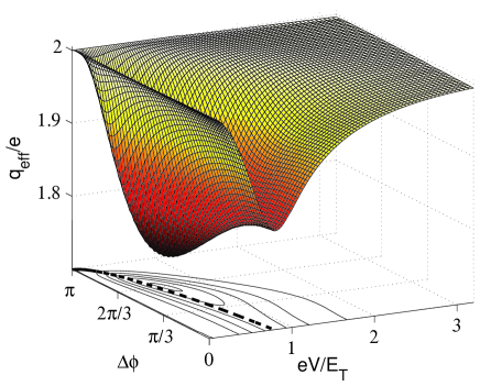
Figure 2: (Color online): Effective charge $q_{\rm eff}$ vs voltage and $\Delta\phi$. The voltage at which the minimum $q_{\rm eff}$ is obtained follows the phase-dependent minigap in the SNS system (bold dashed black curve). Note that the junction undergoes a $\pi$-transition, in which the supercurrent changes its sign, at $eV\approx 2E_{T}$.T. T. Heikkilä et al. (2002); Huang et al. (2002)

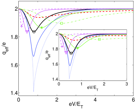
Figure 3: (Color online): Effective charge $q_{\rm eff}$ vs $eV$ for $\Delta\phi=0$ (main figure) and $\Delta\phi=2\pi/3$ (inset). The cross section $A_{c}$ is close to $0$ (blue dotted), $A/4$ (blue solid), $A$ (black bold $\circ$), $4A$ (red dashed) and for these curves $L_{1,2,3}=L$. The values for $L_{3}$ are $1/8$ (green dash-dotted $\Box$), $1/2$ (green solid $\ast$), $2$ (magenta solid $\bigtriangledown$), $4$ (magenta dashed $+$) times $L_{1,2}=L$ with $A_{c}=A$; $E_{T}=\hbar D/L^{2}$. For $\Delta\phi=2\pi/3$, the minima of $q_{\rm eff}$ occur at lower $V$ and except for the curves for $A_{c}=0$ and $L_{3}=L/8$, the dips are deeper than for $\Delta\phi=0$. Note the different energy scales on the x-axes in the inset and in the main figure.

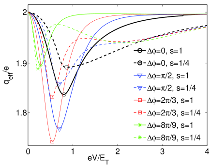
Figure 4: (Color online): Effective charge $q_{\rm eff}$ for different values of phase difference in left-right symmetric ($s=1$) and asymmetric ($s=1/4$) structures.

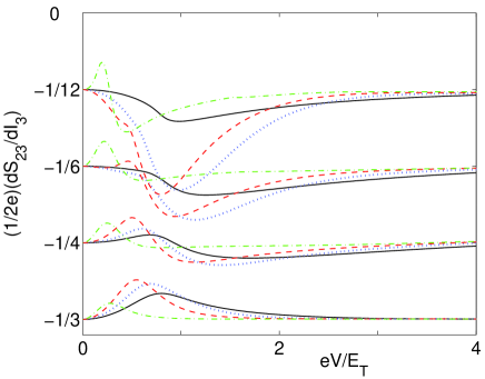
Figure 5: (Color online): Normalized differential cross correlations $(1/2e)(\mathrm{d}S_{23}/\mathrm{d}\bar{I}_{3})$ vs $eV$, for $\Delta\phi=0$ (black solid), $\Delta\phi=\pi/2$ (blue dotted), $\Delta\phi=2\pi/3$ (red dashed), $\Delta\phi=8\pi/9$ (green dash-dotted) and $s=1/4,1/2,3/4,1$ for the curves from top to bottom. The cross correlations related to the opposite wire are directly obtained from $S_{13}=-S_{23}-S_{33}$. The results for $S_{23}$ and the symmetry parameter $s$ are identical for those for $S_{13}$ and $2-s$ by the symmetry of $S_{ij}$ under the reversal of the phase gradient.

In Fig. 3, $q_{\rm eff}$ vs $eV$ is plotted for a vanishing $\Delta\phi$ and for different cross sections $A_{c}$ and lengths $L_{3}$ of the control wire, with given $E_{T}=\hbar D/L^{2}$. The influence of a finite $\Delta\phi$ is exemplified in the inset, where the results for the same parameters as in the Fig. 3, but for $\Delta\phi=2\pi/3$, have been plotted. The behavior of the supercurrent in somewhat similar situations has been studied earlier in Refs. T. T. Heikkilä et al., 2002 and Huang et al., 2002. For $A_{c}\rightarrow 0$, the voltage at which the minimum $q_{\rm eff}$ is obtained exactly coincides with the phase-dependent minigap in the SNS system. Generally, enlarging the width of the control wire or varying the lengths away from the symmetric case $L_{1,2,3}=L$ tends to make the dip shallower. With $L_{1,2}=L$ and $L_{3}$ smaller (larger) than $L$, the minimum in $q_{\rm eff}$ is shifted to higher (lower) voltages. This is in agreement with the conclusion that the dip is caused by the anticorrelation between subsequent Andreev pairs as the correlations of the pairs manifest themselves at the length scale $\sim(\hbar D/\varepsilon)^{1/2}$.

Under the sign reversal of $\Delta\phi$, at energies below $eV$, the dissipative and superconducting parts of the spectral charge current $j_{T}$ remain invariant.Heikkilä et al. (2003) A direct calculation shows that also $S_{ij}$ is invariant under the sign reversal of $\Delta\phi$ (also in asymmetric structures). This means that the quasiparticle current is in no way correlated with the supercurrent flowing in the system, although the presence of the latter changes the correlations in the previous. Hence in the left-right symmetric structures, we have $S_{13}=S_{23}=-S_{33}/2$ through current conservation. Note that if the supercurrent would be replaced by a dissipative current, the cross correlations would depend on the relative signs between $\bar{I}_{3}$ and the ”circulating” current $\bar{I}_{1}-\bar{I}_{2}$. In order to study the effect of asymmetry, we introduce a symmetry parameter, $0<s<2$, measuring the distance between the wire $3$ and $T_{1}$ such that $L_{1}/s=L_{2}/(2-s)=L_{3}=L$. The symmetric system described above corresponds thus to $s=1$. The same results for $q_{\rm eff}$ apply for the symmetry parameters $s$ and $2-s$ as $q_{\rm eff}$ is invariant under the change of the sign of $\Delta\phi$. Hence we restrict ourselves to $s\leq 1$ without loss of generality. In Fig. 4, we have calculated $q_{\rm eff}$, i.e., a normalized autocorrelation function by varying $s$ and $\Delta\phi$. With decreasing $s$, the coherence in the control wire increases as the other superconducting terminal is brought closer to it. At voltages higher than $E_{T}/e$, but in the region where the coherence is not fully suppressed, the enhanced coherence gives rise to the long tails with $q_{\rm eff}<2e$ in Fig. 4. However, at voltages near the minimum of $q_{\rm eff}$, decreasing $s$ suppresses the dip.

Figure 5 represents the normalized differential cross correlations $(1/2e)(\textrm{d}S_{23}/\textrm{d}\bar{I}_{3})$. In the lowest curves for the symmetrical case, $s=1$, we have $(1/2e)(\textrm{d}S_{23}/\textrm{d}\bar{I}_{3})=-q_{\rm eff}/6e$. In the incoherent region $eV\gg E_{T}$, the absolute value of $S_{23}$ diminishes linearly with decreasing $s$, as one may anticipate on the basis of the Kirchoff rules. In the coherent regime, $\textrm{d}S_{23}/\textrm{d}\bar{I}_{3}$ reflects, e.g., the relative changes in $\textrm{d}\bar{I}_{2}/\textrm{d}V$ and $\textrm{d}\bar{I}_{3}/\textrm{d}V$ with $V$. In the symmetric case, these relative changes have equal magnitudes. If the former exhibits a larger change than the latter, $(1/2e)(\textrm{d}S_{23}/\textrm{d}\bar{I}_{3})$ may obtain larger negative values than in the incoherent regime. With a finite supercurrent these dips correspond to the processes in which two electrons are injected from the normal reservoir and an Andreev pair enters the superconductor $T_{2}$.

In conclusion, we have found a physically transparent and computationally efficient way to calculate the full phase and voltage dependence of the noise correlations in mesoscopic diffusive wires in the presence of supercurrent. We found that the strength of the anticorrelations between the Andreev pairs flowing in the structure is closely related to the magnitude (but not to the sign) of the spectral supercurrent and the variations in the local density of states.

We acknowledge W. Belzig, M. Houzet, and F. Pistolesi for discussions and Center for Scientific Computing for computing resources. M.P.V.S. acknowledges the financial support of Magnus Ehrnrooth Foundation and the Foundation of Technology (TES, Finland). P. V. thanks the Finnish Cultural Foundation and T.T.H. the Academy of Finland for funding.

References

Ya. M. Blanter and M.
Büttiker (2001)
Ya. M. Blanter and
M. Büttiker, Phys.
Rep. 336, 1
(2001).
K. A. Muttalib et al. (2003)
K. A. Muttalib,
P. Wölfle, and
V. A. Gopar, Ann. Phys.
308, 156 (2003).
Stenberg and Särkkä (2006)
M. P. V. Stenberg
and
J. Särkkä,
Phys. Rev. B 74,
035327 (2006).
Reulet et al. (2003)
B. Reulet,
A. A. Kozhevnikov,
D. E. Prober,
W. Belzig, and
Y. V. Nazarov,
Phys. Rev. Lett. 90,
066601 (2003).
X. Jehl et al. (2000)
X. Jehl, M.
Sanquer, R. Calemczuk, and
D. Mailly, Nature
(London) 405, 50
(2000).
Kozhevnikov et al. (2000)
A. A. Kozhevnikov,
R. J. Schoelkopf,
and D. E.
Prober, Phys. Rev. Lett.
84, 3398 (2000).
F. Lefloch et al. (2003)
F. Lefloch, C.
Hoffmann, M. Sanquer, and
D. Quirion, Phys. Rev.
Lett. 90, 067002
(2003).
Belzig and Nazarov (2001)
W. Belzig and
Y. V. Nazarov,
Phys. Rev. Lett. 87,
067006 (2001).
Stenberg and Heikkilä (2002)
M. P. V. Stenberg
and T. T.
Heikkilä, Phys. Rev. B
66, 144504
(2002).
Houzet and Pistolesi (2004)
M. Houzet and
F. Pistolesi,
Phys. Rev. Lett. 92,
107004 (2004).
Nazarov and Bagrets (2002)
Y. V. Nazarov and
D. A. Bagrets,
Phys. Rev. Lett. 88,
196801 (2002).
Samuelsson and Büttiker (2002)
P. Samuelsson and
M. Büttiker,
Phys. Rev. B 66,
201306(R) (2002).
P. Virtanen and T. T.
Heikkilä (2006)
P. Virtanen and
T. T. Heikkilä, New J.
Phys. 8, 50
(2006).
W. Belzig and P. Samuelsson (2003)
W. Belzig and
P. Samuelsson, Europhys.
Lett. 64, 253
(2003).
Bezuglyi et al. (2004)
E. V. Bezuglyi,
E. N. Bratus’,
V. S. Shumeiko,
and V. Vinokur,
Phys. Rev. B 70,
064507 (2004).
Zhou et al. (1998)
F. Zhou,
P. Charlat,
B. Spivak, and
B. Pannetier,
J. Low Temp. Phys. 110,
841 (1998).
L. S. Levitov et al. (1996)
L. S. Levitov,
H. W. Lee, and
G. B. Lesovik, J. Math.
Phys. (N.Y.) 37, 4845
(1996).
Yu. V. Nazarov, Ann. Phys. (Berlin)
Yu. V. Nazarov, Ann. Phys. (Berlin) 8, SI-193 (1999).
W. Belzig in Quantum Noise in Mesoscopic Physics, edited by Yu.
V. Nazarov (Kluwer, Dordrecht, 2003)
W. Belzig in Quantum Noise in Mesoscopic Physics, edited by Yu. V.
Nazarov (Kluwer, Dordrecht, 2003), p. 463.
W. Belzig et al. (1999)
W. Belzig, F.
K. Wilhelm, C. Bruder,
G. Schön, and
A. D. Zaikin,
Superlattices Microstruct. 25,
1251 (1999).
Usadel (1970)
K. D. Usadel,
Phys. Rev. Lett. 25,
507 (1970).
Nazarov (1999)
Y. V. Nazarov,
Superlattices Microstruct. 25,
1221 (1999).
23
There is a misprint in this formula in Ref. Houzet and Pistolesi, 2004.
Samuelsson et al. 2004
P. Samuelsson,
W. Belzig, and
Y. V. Nazarov,
Phys. Rev. Lett. 92,
196807 (2004).
T. T. Heikkilä et al. 2002
T. T. Heikkilä,
J. Särkkä, and
F. K. Wilhelm, Phys. Rev.
B 66, 184513
(2002).
Huang et al. 2002
J. Huang,
F. Pierre,
T. T. Heikkilä,
F. K. Wilhelm,
and N. O. Birge,
Phys. Rev. B 66,
020507(R) (2002).
Heikkilä et al. 2003
T. T. Heikkilä,
T. Vänskä,
and F. K.
Wilhelm, Phys. Rev. B
67, 100502(R)
(2003).