Charge transport in a Tomonaga-Luttinger liquid: effects of pumping and bias

Abstract

We study the current produced in a Tomonaga-Luttinger liquid by an applied bias and by weak, point-like impurity potentials which are oscillating in time. We use bosonization to perturbatively calculate the current up to second order in the impurity potentials. In the regime of small bias and low pumping frequency, both the DC and AC components of the current have power law dependences on the bias and pumping frequencies with an exponent $2K-1$ for spinless electrons, where $K$ is the interaction parameter. For $K<1/2$, the current grows large for special values of the bias. For non-interacting electrons with $K=1$, our results agree with those obtained using Floquet scattering theory for Dirac fermions. We also discuss the cases of extended impurities and of spin-1/2 electrons.

I Introduction

The conductance of electrons in a quantum wire has been studied extensively in recent years both theoretically datta ; imry and experimentally tarucha ; liang ; bkane ; yacoby ; auslaender ; reilly . For a wire in which only one channel is available to the electrons and the transport is ballistic (i.e., there are no impurities inside the wire, and there is no scattering from phonons or from the contacts between the wire and its leads), the conductance is given by $G=2e^{2}/h$ for infinitesimal bias. However, if there is an impurity inside the wire which scatters the electrons, then the conductance is reduced. For a $\delta$-function impurity with strength $U$, we obtain $G=(2e^{2}/h)~{}(1-U^{2}/v_{F}^{2}),$ to lowest order in $U$, where $v_{F}$ is the Fermi velocity of the electrons. In the presence of interactions between the electrons, the impurity strength $U$ effectively becomes a function of the length scale through a renormalization group (RG) equation kane ; furusaki . The RG flow has to be cut-off at the smallest of the three length scales of the system, namely, the wire length, the thermal length which is inversely proportional to the temperature, and a length which is inversely proportional to the bias voltage $V_{bias}$. If the latter length scale is the smallest of the three, then the effective value of the impurity strength is given by $UV_{bias}^{K-1}$, where $K$ is a parameter related to the strength of the interactions between the electrons as we will see later. Hence the correction to the conductance due to the combined effect of the impurity and the interactions is given by $\Delta G\sim U^{2}V_{bias}^{2K-2}$.

The phenomenon of charge pumping and rectification by oscillating potentials applied to certain points in a system has also been studied theoretically [11-38] and experimentally switkes ; taly1 ; cunningham ; taly2 ; leek . For the case of non-interacting electrons, theoretical studies have used adiabatic scattering theory avron ; entin1 ; entin2 , Floquet scattering theory moskalets ; kim , variations of the non-equilibrium Green function formalism wang ; arrachea ; torres , and the equation of motion approach agarwal . The case of interacting electrons has also been studied, using a RG method for weak interactions das , and the method of bosonization for arbitrary interactions [45-55]. The analytical methods used in the two cases typically treat the electrons in quite different ways, with a non-relativistic Schrödinger equation or a tight-binding model on a lattice being used in the non-interacting case, and a massless Dirac model followed by bosonization being used in the interacting case.

A clear comparison between the non-interacting and interacting cases does not seem to have been made before. We plan to fill this gap in this paper and will study the effects of electron-electron interactions (of arbitrary repulsive strength) on the DC and AC components of the current in a system with a bias and time-dependent impurities.

In Sec. II, we discuss a massless Dirac model for non-interacting electrons in the presence of several point-like impurities. We use Floquet scattering theory moskalets ; kim to study the pumped and bias current in this model. In Sec. III, we first review the calculation of the backscattered current. Using bosonization gogolin ; rao ; giamarchi , we then compute the DC and AC components of the current up to second order in the impurity potentials feldman1 ; makogon1 . We show that these reduce to the results obtained using Floquet scattering theory for the non-interacting case. The cases of extended impurities makogon2 and of spin-1/2 electrons are discussed briefly. We summarize our results in Sec. IV. We will consider infinitely long wires and zero temperature throughout the paper; hence the relevant energy scales in the problem are set only by the bias and the pumping frequency.

II Massless Dirac model with impurities

In this section we consider a spinless and massless Dirac fermion with no interactions between the fermions, and use the Floquet scattering theory to compute the total current. The Hamiltonian in the presence of several point-like impurities is given by $\hat{H}=\hat{H}_{0}+\hat{H}_{imp}$, where

$$\hat{H}_{0} = \int dx~{}iv_{F}~{}(-~{}\psi_{R}^{\dagger}\frac{\partial\psi_{R}}{\partial x}~{}+~{}\psi^{\dagger}_{L}\frac{\partial\psi_{L}}{\partial x}),$$

$$\hat{H}_{imp} = \int dx~{}\sum_{p}~{}\delta(x-x_{p})~{}U_{p}(t)~{}\psi^{\dagger}(x)\psi(x),$$

$$\psi(x) = \psi_{R}(x)~{}e^{ik_{F}x}~{}+~{}\psi_{L}(x)~{}e^{-ik_{F}x},$$ (1)

where $\psi_{L}$ and $\psi_{R}$ are the fermionic field operators of the left and right moving electrons, $v_{F}$ is the Fermi velocity, and $k_{F}$ is the Fermi wavenumber which originates from some underlying microscopic model. For instance, one may have a system of non-relativistic electrons with a Fermi energy $E_{F}=k_{F}^{2}/(2m)$ and $v_{F}=k_{F}/m$. (We are setting Planck’s constant $\hbar$ equal to unity). The Hamiltonian $\hat{H}_{0}$ is obtained by linearizing the dispersion around the two Fermi points given by $k=\pm k_{F}$. $\hat{H}_{imp}$ arises from the time-dependent impurities which have strengths $U_{p}(t)$; this Hamiltonian couples left and right moving fields since

$$\psi^{\dagger}\psi~{}=~{}\psi_{R}^{\dagger}\psi_{R}~{}+~{}\psi_{L}^{\dagger}\psi_{L}~{}+~{}\psi_{R}^{\dagger}\psi_{L}e^{-i2k_{F}x}~{}+~{}\psi_{L}^{\dagger}\psi_{R}e^{i2k_{F}x}.$$ (2)

We will assume that

$$U_{p}(t)~{}=~{}U_{p}~{}\cos(\omega t+\phi_{p}),$$ (3)

i.e., all impurities vary harmonically in time with the same frequency $\omega$. We will now use Floquet scattering theory and carry out a perturbative expansion in the dimensionless quantities $U_{p}/v_{F}$.

The equations of motion in the presence of a single $\delta$-function impurity $\delta(x-x_{p})U_{p}\cos(\omega t+\phi_{p})$ is as follows:

$$i~{}\frac{\partial\psi_{R}}{\partial t}~{}+~{}iv_{F}~{}\frac{\partial\psi_{R}}{\partial x}$$

$$=~{}\delta(x-x_{p})~{}U_{p}\cos(\omega t+\phi_{p})~{}(\psi_{R}~{}+~{}\psi_{L}e^{-i2k_{F}x_{p}}),$$

$$i~{}\frac{\partial\psi_{L}}{\partial t}~{}-~{}iv_{F}~{}\frac{\partial\psi_{L}}{\partial x}$$

$$=~{}\delta(x-x_{p})~{}U_{p}\cos(\omega t+\phi_{p})~{}(\psi_{L}~{}+~{}\psi_{R}e^{i2k_{F}x_{p}}).$$

If we define the linear combinations $\psi_{+}=\psi_{R}e^{ik_{F}x_{p}}+\psi_{L}e^{-ik_{F}x_{p}}$ and $\psi_{-}=\psi_{R}e^{ik_{F}x_{p}}-\psi_{L}e^{-ik_{F}x_{p}}$, we find that

$$i~{}\frac{\partial\psi_{-}}{\partial t}~{}+~{}iv_{F}~{}\frac{\partial\psi_{+}}{\partial x}=0,$$

$$i~{}\frac{\partial\psi_{+}}{\partial t}~{}+~{}iv_{F}~{}\frac{\partial\psi_{-}}{\partial x}=2\delta(x-x_{p})U_{p}\cos(\omega t+\phi_{p})~{}\psi_{+}.$$

By integrating over a little region from $x_{p}-\epsilon$ to $x_{p}+\epsilon$, we find that $\psi_{+}$ is continuous at the point $x=x_{p}$, while $\psi_{-}$ has a discontinuity given by

$$iv_{F}~{}[\psi_{-}(x_{p}+\epsilon)~{}-~{}\psi_{-}(x_{p}-\epsilon)]~{}=~{}2U_{p}\cos(\omega t+\phi_{p})~{}\psi_{+}(x_{p}).$$ (6)

We would like to note here that it is necessary to retain the terms $\psi_{R}^{\dagger}\psi_{R}+\psi_{L}^{\dagger}\psi_{L}$ in Eq. (2) in order to have continuity of $\psi_{+}$. In some papers, these terms are not taken into consideration. One then runs into the mathematical peculiarity that $\psi_{+}$ and $\psi_{-}$ are both discontinuous at $x=x_{p}$, and the discontinuity is taken to be proportional to their values at that point; but those values are actually ill-defined due to the discontinuity.

We can now solve Eqs. (II) along with the boundary conditions in Eq. (6). For a single $\delta$-function impurity oscillating with frequency $\omega$ at $x=x_{p}$, let us consider a wave coming from the left ($x<x_{p}$) with energy $E_{0}$ and unit amplitude. Note that we are measuring energies with respect to a Fermi energy, so that $E_{0}=0$ corresponds to a fermion at the Fermi energy. Due to the oscillating impurity potential, the wave will be reflected back to the left with energy $E_{n}\equiv E_{0}+n\omega$ and amplitude $S_{LL}(E_{n},E_{0})$, or transmitted to the right ($x>x_{p}$) with energy $E_{n}$ and amplitude $S_{RL}(E_{n},E_{0})$, where $n=0,\pm 1,\pm 2,\cdots$ defines the Floquet side bands moskalets . Note that since we are considering a Dirac fermion, there is no upper or lower bound to the energy $E_{n}$, and the velocity $v_{F}$ is independent of the energy. (This is unlike the case of a non-relativistic fermion or a fermion on a lattice where there is a lower or upper bound to the energy, and the velocity is a function of the energy). To be explicit, the wave function is given by

$$\psi_{R} = e^{i(k_{0}x-E_{0}t)}\quad{\rm for}\quad x<x_{p}~{},$$

$$= \sum_{n}~{}S_{RL}(E_{n},E_{0})~{}e^{i(k_{n}x-E_{n}t)}\quad{\rm for}\quad x>x_{p}~{},$$

$$\psi_{L} = \sum_{n}~{}S_{LL}(E_{n},E_{0})~{}e^{i(-k_{n}x-E_{n}t)}\quad{\rm for}\quad x<x_{p}~{},$$ (7)

$$= 0\quad{\rm for}\quad x>x_{p}~{},$$

where $k_{n}=E_{n}/v_{F}$. Similarly, we can consider a wave coming from the right with energy $E_{0}$ and unit amplitude; it will be reflected back to the right with amplitude $S_{RR}(E_{n},E_{0})$ or transmitted to the left with amplitude $S_{LR}(E_{n},E_{0})$. Let us simplify the notation by defining

$$r_{L,n} = S_{LL}(E_{n},E_{0}),\quad t_{L,n}~{}=~{}S_{LR}(E_{n},E_{0}),$$

$$t_{R,n} = S_{RL}(E_{n},E_{0}),\quad r_{R,n}~{}=~{}S_{RR}(E_{n},E_{0}).$$ (8)

Due to unitarity, we have the relations

$$\sum_{n}~{}[~{}|r_{L,n}|^{2}~{}+~{}|t_{R,n}|^{2}~{}] = 1,$$

$$\sum_{n}~{}[~{}|r_{R,n}|^{2}~{}+~{}|t_{L,n}|^{2}~{}] = 1.$$ (9)

The different Floquet scattering amplitudes $r_{\alpha,n}$ and $t_{\alpha,n}$ can be found by using the boundary conditions in Eq. (6). We will consider the case of several impurities labeled by the index $p$ as in Eq. (1). To simplify our calculations, we will assume that $\omega(x_{p}-x_{r})/v_{F}$ and $E_{0}(x_{p}-x_{r})/v_{F}$ are small for all pairs of impurities $p$ and $r$; the first condition corresponds to the adiabatic limit, while the second condition implies that we are only considering states close to the Fermi energy. Keeping terms only up to first order in $U_{p}/v_{F}$, we find that only the first Floquet side bands are excited, and

$$t_{L,1} = t_{R,1}~{}=~{}-~{}\frac{i}{2v_{F}}~{}\sum_{p}~{}U_{p}~{}e^{-i\phi_{p}},$$

$$t_{L,-1} = t_{R,-1}~{}=~{}-~{}\frac{i}{2v_{F}}~{}\sum_{p}~{}U_{p}~{}e^{i\phi_{p}}.$$

$$r_{L,1} = -~{}\frac{i}{2v_{F}}~{}\sum_{p}~{}U_{p}~{}e^{i(2k_{F}x_{p}-\phi_{p})},$$

$$r_{L,-1} = -~{}\frac{i}{2v_{F}}~{}\sum_{p}~{}U_{p}~{}e^{i(2k_{F}x_{p}+\phi_{p})}.$$

$$r_{R,1} = -~{}\frac{i}{2v_{F}}~{}\sum_{p}~{}U_{p}~{}e^{i(-2k_{F}x_{p}-\phi_{p})},$$

$$r_{R,-1} = -~{}\frac{i}{2v_{F}}~{}\sum_{p}~{}U_{p}~{}e^{i(-2k_{F}x_{p}+\phi_{p})},$$ (10)

We also find that the unitarity relations in Eq. (9) are satisfied up to second order in $U_{p}/v_{F}$, and therefore $t_{L,0}$ and $t_{R,0}$ are given by

$$|t_{L,0}|^{2} = 1-|r_{R,1}|^{2}-|r_{R,-1}|^{2}-|t_{L,1}|^{2}-|t_{L,-1}|^{2},$$

$$|t_{R,0}|^{2} = 1-|r_{L,1}|^{2}-|r_{L,-1}|^{2}-|t_{R,1}|^{2}-|t_{R,-1}|^{2},$$

to that order in $U_{p}/v_{F}$. Note that the amplitudes given in Eqs. (10-LABEL:t0) are all independent of $E_{0}$ under the approximations that we have made.

The dc part of the current in, say, the right lead is given by moskalets

$$I_{R,dc} = q~{}\int_{-\infty}^{\infty}\frac{dE_{0}}{2\pi}~{}\sum_{n}~{}[~{}|r_{R,n}|^{2}~{}\{f_{R}(E_{0})-f_{R}(E_{n})\}$$

$$\quad\quad\quad\quad\quad\quad~{}+~{}|t_{R,n}|^{2}~{}\{f_{L}(E_{0})-f_{R}(E_{n})\}~{}],$$

where $q$ is the charge of the electron, and $f_{\alpha}(E)=1/[e^{(E-\mu_{\alpha})/k_{B}T}+1]$ is the Fermi function in the lead $\alpha$. At zero temperature, $f_{\alpha}(E)=\theta(\mu_{\alpha}-E)$, where $\theta(E)=1$ for $E>0$ and 0 for $E<0$. Note that in a non-relativistic system, an expression like (LABEL:irdc) would contain ratios of velocities $v_{n}/v_{0}$. Since we are considering a massless Dirac fermion here, the velocity is independent of the energy, and $v_{n}/v_{0}=1$ for all $n$.

Let us define a frequency in terms of the bias voltage, $\omega_{0}=qV_{bias}=\mu_{R}-\mu_{L}$. We will assume the bias to be small so that $\omega_{0}(x_{r}-x_{p})/v_{F}$ is small for all values of $p$ and $r$. Using Eqs. (10-LABEL:t0), we find, up to second order in $U_{p}/v_{F}$, that

$$I_{R,dc} = -~{}\frac{q\omega_{0}}{2\pi}~{}[~{}|t_{R,0}|^{2}~{}+~{}|t_{R,1}|^{2}~{}+~{}|t_{R,-1}|^{2}~{}]$$ (13)

$$+~{}\frac{q\omega}{2\pi}~{}[~{}|t_{R,1}|^{2}-|t_{R,-1}|^{2}+|r_{R,1}|^{2}-|r_{R,-1}|^{2}~{}]$$

$$= -~{}\frac{q\omega_{0}}{2\pi}~{}+~{}\frac{q\omega_{0}}{4\pi v_{F}^{2}}~{}[\sum_{p}~{}U_{p}^{2}$$

$$\quad\quad\quad\quad~{}+~{}2~{}\sum_{p<r}~{}U_{p}U_{r}\cos(2k_{F}x_{rp})\cos(\phi_{rp})]$$

$$-~{}\frac{q\omega}{2\pi v_{F}^{2}}~{}\sum_{p<r}~{}U_{p}U_{r}~{}\sin(2k_{F}x_{rp})\sin(\phi_{rp}),$$

where $x_{rp}=x_{r}-x_{p}$ and $\phi_{rp}=\phi_{r}-\phi_{p}$. Eq. (13) shows the effects of a bias ($\omega_{0}$) and harmonically oscillating potentials ($\omega$). For the pure pumping case with $\omega_{0}=0$, Eq. (13) agrees with the results presented in Ref. agarwal ; note that the pumped current depends on $\sin(\phi_{rp})$.

It is interesting to note that the first term is just the ballistic conductance of a clean wire multiplied by the bias, the second term is a correction to the clean case because of the presence of impurities, and the third term is the pumped current. In the non-interacting case, the bias component and the pumped component separate out, but for the interacting case, the current involves powers of $\omega_{0}\pm\omega$.

III Bosonization calculation of backscattered current

III.1 Backscattering current operator

We now compute the current in a system of interacting electrons using the backscattering current operator introduced in Refs. chamon1 ; chamon2 ; sharma ; feldman1 .

Let us take the impurity potentials to be absent at time $t=-\infty$; then they are gradually switched on. At the initial time, $H_{0}$ commutes with the number operators of the left moving and right moving fermions, $\hat{N}_{L}$ and $\hat{N}_{R}$ respectively. In the absence of any impurity potentials, all the right movers originate in the left reservoir which is maintained at the chemical potential $\mu_{L}$, and all the left movers originate in the right reservoir maintained at the chemical potential $\mu_{R}$. Hence, the system is initially described in the grand canonical ensemble by the chemical potentials $\mu_{L}$ and $\mu_{R}$ which are the coefficients of the number operators $\hat{N}_{L}$ and $\hat{N}_{R}$ respectively. We will work in the interaction representation, taking the chemical potentials to be part of the interaction. This introduces time dependences into the fermionic operators $\psi_{L}\to\psi_{L}e^{i\mu_{L}t}$ and and $\psi_{R}\to\psi_{R}e^{i\mu_{R}t}$. The operators $\psi_{L}^{\dagger}\psi_{R}$ and $\psi_{R}^{\dagger}\psi_{L}$ appearing in in $H_{imp}$ (see Eqs. (1) and (2)) therefore pick up factors of $e^{\pm i\omega_{0}t}$.

If there were no impurities, there would be a current flowing to the left given by $I_{0}=q^{2}V_{bias}/(2\pi)=q\omega_{0}/(2\pi)$. In the presence of impurities, some of this current is backscattered to the right. The total current flowing to the right is given by $I=-I_{0}+I_{bs}$, where $I_{bs}$ is the correction to the current due to backscattering by the impurities. The backscattered current is defined as

$$\hat{I}_{bs}(t) = q~{}\frac{d\hat{N}_{R}}{dt}~{}=~{}-iq~{}[\hat{N}_{R}~{},~{}\hat{H}_{imp}~{}]$$

$$= iq~{}\sum_{p}~{}U_{p}(t)~{}[~{}\psi^{\dagger}_{L}\psi_{R}~{}e^{i(\omega_{0}t+2k_{F}x_{p})}-H.c.~{}].$$

The backscattered current at any time $t$ is given by

$$\langle\hat{I}_{bs}\rangle=\langle 0|~{}S(-\infty;t)~{}\hat{I}_{bs}(t)~{}S(t;-\infty)~{}|0\rangle,$$ (15)

where $|0\rangle$ denotes the initial state at $t\to-\infty$, and $S$ is the scattering matrix arising due to the impurities,

$$S(t;-\infty)~{}=~{}S^{\dagger}(-\infty;t)~{}=~{}T~{}\exp[-i~{}\int_{-\infty}^{t}dt^{\prime}~{}\hat{H}_{imp}(t^{\prime})].$$ (16)

We define a backscattering operator

$$\hat{B}_{p}(t)~{}=~{}U_{p}(t)~{}\psi^{\dagger}_{L}\psi_{R}~{}e^{i(\omega_{0}t+2k_{F}x_{p})}.$$ (17)

In terms of this, $\hat{I}_{bs}(t)=iq\sum_{p}[\hat{B}_{p}(t)-H.c.]$, while $S(t,-\infty)=1-i\sum_{p}\int_{-\infty}^{t}dt^{\prime}[\hat{B}_{p}(t^{\prime})+H.c.]$ to first order in $U_{p}$. Thus

$$I_{bs} = q~{}\sum_{p,r}~{}\int_{-\infty}^{t}dt^{\prime}~{}\langle 0|~{}[~{}\hat{B}_{p}(t^{\prime})\hat{B}_{r}^{\dagger}(t)-\hat{B}_{p}^{\dagger}(t^{\prime})\hat{B}_{r}(t)~{}]$$ (18)

$$\quad\quad\quad\quad\quad\quad\quad\quad\quad+~{}H.c.~{}|0\rangle$$

to second order in $U_{p}$.

III.2 Bosonization

In one dimension, it is known that a large class of fermion systems which are gapless and have a low-energy dispersion which is linear can be written in terms of gapless bosonic systems gogolin ; rao ; giamarchi . These systems are called Tomonaga-Luttinger liquids; for spinless fermions, they are characterized by an interaction parameter $K$ and a velocity $v$. Non-interacting fermions have $K=1$ and $v=v_{F}$, while $K<1$ corresponds to repulsive interactions between the fermions. To be specific, consider a system with short-range density-density interactions of the form

$$H_{int}~{}=~{}\frac{1}{2}~{}\int\int~{}dxdy~{}\rho(x)V(x-y)\rho(y),$$ (19)

where $V(x)$ is a real and even function of $x$, and the density $\rho=\psi^{\dagger}\psi$ is given in Eq. (2). We can write Eq. (19) in a simple way if $V(x)$ is so short ranged that the arguments $x$ and $y$ of the two density fields can be set equal to each other wherever possible. Using the anticommutation relations between the fermion fields, we obtain

$$H_{int}~{}=~{}g_{2}~{}\int~{}dx~{}\psi_{R}^{\dagger}\psi_{R}\psi_{L}^{\dagger}\psi_{L},$$ (20)

where $g_{2}$ is related to the Fourier transform of $V(x)$ as $g_{2}={\tilde{V}}(0)-{\tilde{V}}(2k_{F})$. Defining a parameter $\gamma=g_{2}/(2\pi v_{F})$, we have the relations

$$K = \left(\frac{1-\gamma}{1+\gamma}\right)^{1/2},$$

$$v = v_{F}~{}(1-\gamma^{2})^{1/2}.$$ (21)

In the absence of impurities, the bosonic action is given by

$$S~{}=~{}\int dtdx\left[~{}\frac{1}{2v}~{}\left(\frac{\partial\phi}{\partial t}\right)^{2}~{}-~{}\frac{v}{2}~{}\left(\frac{\partial\phi}{\partial x}\right)^{2}~{}\right].$$ (22)

Bilinears in fermion operators can be written in terms of bosons and Klein operators gogolin ; rao ; giamarchi , such as

$$\hat{\psi}_{R}^{\dagger}\hat{\psi}_{L} = \frac{1}{2\pi\alpha}~{}\hat{\eta}_{R}^{\dagger}\hat{\eta}_{L}~{}e^{i2\sqrt{\pi K}\hat{\phi}},$$

$$\hat{\psi}_{L}^{\dagger}\hat{\psi}_{R} = \frac{1}{2\pi\alpha}~{}\hat{\eta}_{L}^{\dagger}\hat{\eta}_{R}~{}e^{-i2\sqrt{\pi K}\hat{\phi}},$$ (23)

where $\eta_{R}$ and $\eta_{L}$ are the Klein operators, and $\alpha$ is a short distance cut-off. We then obtain the ground state expectation value of products of four fermion operators as in Eq. (18), namely,

$$\langle 0|~{}\psi_{R}^{\dagger}(x_{p},t^{\prime})\psi_{L}(x_{p},t^{\prime})\psi_{L}^{\dagger}(x_{r},t)\psi_{R}(x_{r},t)~{}|0\rangle$$ (24)

$$= \frac{\alpha^{2K-2}}{(2\pi)^{2}~{}[(x_{p}-x_{r})^{2}~{}-~{}(v(t^{\prime}-t)-i\alpha)^{2}]^{K}}$$

for all values of $K$.

For the non-interacting case with $K=1$, we can evaluate the above ground state expectation value directly without using bosonization. We use the second quantized expressions for the fermion fields,

$$\psi_{R} = \int_{-\infty}^{\infty}~{}\frac{dk}{2\pi}~{}a_{Rk}~{}e^{ik(x-v_{F}t)},$$

$$\psi_{L} = \int_{-\infty}^{\infty}~{}\frac{dk}{2\pi}~{}a_{Lk}~{}e^{ik(-x-v_{F}t)},$$ (25)

where the creation and annihilation operators satisfy the anticommutation relations $\{a_{Rk},a_{Rk^{\prime}}^{\dagger}\}=\{a_{Lk},a_{Lk^{\prime}}^{\dagger}\}=2\pi\delta(k-k^{\prime})$. The ground state $|0\rangle$ is annihilated by $a_{Rk},a_{Lk}$ for $k>0$ and by $a_{Rk}^{\dagger},a_{Lk}^{\dagger}$ for $k<0$. We then find that the ground state expectation value agrees with the result given in Eq. (24) for $K=1$ and $v=v_{F}$.

In general, the backscattered current has two parts: one independent of time which we call $I_{dc}$, and the other varying with time, with frequency $2\omega$ to second order in $U_{p}$, which we call $I_{ac}$. $I_{ac}$ does not contribute to any charge transfer as its average over a cycle is zero. In the next few subsections, we calculate the expectation value of the backscattered current for various cases and study them in different limits. To simplify our calculations, we again assume that $\omega x_{rp}/v$ and $\omega_{0}x_{rp}/v$ are small and that $\omega\geq 0$. It will be convenient to define the combinations

$$\omega_{+}~{}=~{}\omega_{0}~{}+~{}\omega,\quad{\rm and}\quad\omega_{-}~{}=~{}\omega_{0}~{}-~{}\omega.$$ (26)

III.3 Single impurity

This case has been discussed in Ref. feldman1 ; we reproduce the results here for the sake of completeness. Some details of the calculations are provided in the Appendix.

$$I_{bs,dc}^{pp} = \frac{qU_{p}^{2}}{8\pi v^{2}\Gamma(2K)}~{}\left(\frac{\alpha}{v}\right)^{2K-2}$$

$$\times [sgn(\omega_{+})~{}|\omega_{+}|^{2K-1}~{}+~{}sgn(\omega_{-})~{}|\omega_{-}|^{2K-1}],$$

$$I_{bs,ac}^{pp} = \frac{qU_{p}^{2}}{8\pi v^{2}\Gamma(2K)\cos(\pi K)}~{}\left(\frac{\alpha}{v}\right)^{2K-2}$$

$$\times [sgn(\omega_{+})~{}|\omega_{+}|^{2K-1}$$

$$~{}\times~{}\cos(2\omega t+2\phi_{p}+sgn(\omega_{+})\pi K)$$

$$~{}+~{}sgn(\omega_{-})~{}|\omega_{-}|^{2K-1}$$

$$~{}\times~{}\cos(2\omega t+2\phi_{p}-sgn(\omega_{-})\pi K)],$$

where $sgn(\Omega)\equiv 1$ if $\Omega>0$, $0$ if $\Omega=0$ and $-1$ if $\Omega<0$. In Eqs. (LABEL:idc1-LABEL:iac1), we note that the currents become large in the limit $\omega_{0}\to\pm\omega$ if $K<1/2$. Hence the perturbative expansion in powers of $U_{p}$ breaks down when $\omega_{0}$ is close to $\pm\omega$ feldman1 . The region of validity of the perturbative expansion can be estimated using a RG analysis as discussed below.

Eqs. (LABEL:idc1-LABEL:iac1) imply that for the pure pumping case with $\omega_{0}=0$, $~{}I_{bs,dc}^{pp}=I_{bs,ac}^{pp}=0$. For a single impurity, therefore, charge pumping does not occur, whether or not there are interactions between the electrons. For the pure bias case with $\omega=0$ and $\phi_{p}=0$, we have $~{}I_{bs,dc}^{pp}+I_{bs,ac}^{pp}\sim U_{p}^{2}\omega_{0}^{2K-1}$. Thus the backscattering correction to the conductance given by $-I_{bs,dc}/V_{bias}=-qI_{bs,dc}/\omega_{0}$ is proportional to $U_{p}^{2}V_{bias}^{2K-2}$.

In the presence of both bias and pumping, the correction to the differential conductance $\Delta G=-q\partial I_{bs,dc}/\partial\omega_{0}$ grows large as $U_{p}^{2}|\omega_{\pm}|^{2K-2}$ for $\omega_{+}$ or $\omega_{-}\to 0$. This is consistent with results based on RG calculations kane ; furusaki . Namely, the presence of interactions between the electrons effectively makes the impurity strength $U_{p}$ a function of the length scale; this is described by the RG equation $dU_{p}/d\ln L=(1-K)U_{p}$, to first order in $U_{p}(L)$. Hence the value of $U_{p}(L)$ at a length scale $L$ is related to its value $U_{p}$ defined at a microscopic length scale (say, $\alpha$) as $U_{p}(L)=(L/\alpha)^{1-K}U_{p}$. In our case, the length scale $L$ is set by $v/|\omega_{+}|$ or $v/|\omega_{-}|$. The effective impurity strength $U_{p}(L)$ therefore increases as $(v/|\omega_{\pm}|)^{1-K}U_{p}$ for $\omega_{+}$ or $\omega_{-}\to 0$, and the correction $\Delta G$ grows as $[U_{p}(L)]^{2}\sim U_{p}^{2}|\omega_{\pm}|^{2K-2}$. This divergence must be cut off when $\Delta G$ becomes of order 1, in units of $q^{2}/(2\pi)$. Restoring the appropriate dimensionful quantities, we see that the above RG analysis and perturbative expansion are valid as long as $U_{p}/v<<(\alpha|\omega_{\pm}|/v)^{1-K}$.

III.4 Several impurities

We now consider the case of several impurities located at $x_{p}$ with the phases of the oscillating potentials being $\phi_{p}$. We again define $x_{rp}$ and $\phi_{rp}$ as in Eq. (13). The backscattered current can be written as $I_{bs}=\sum_{p}I_{bs}^{pp}+\sum_{p<r}I_{bs}^{pr}$. The dc and ac parts of $I_{bs}^{pp}$ are given in the previous subsection. Next, we find that

$$I_{bs,dc}^{pr} = \frac{qU_{p}U_{r}}{4\pi v^{2}\Gamma(2K)}\left(\frac{\alpha}{v}\right)^{2K-2}$$

$$\times [sgn(\omega_{+})~{}|\omega_{+}|^{2K-1}\cos(2k_{F}x_{rp}+\phi_{rp})$$

$$+~{}sgn(\omega_{-})~{}|\omega_{-}|^{2K-1}\cos(2k_{F}x_{rp}-\phi_{rp})],$$

$$I_{bs,ac}^{pr} = \frac{qU_{p}U_{r}}{4\pi v^{2}\Gamma(2K)\cos(\pi K)}\left(\frac{\alpha}{v}\right)^{2K-2}\cos(2k_{F}x_{rp})$$

$$\times [sgn(\omega_{+})~{}|\omega_{+}|^{2K-1}$$

$$~{}\times~{}\cos(2\omega t+\phi_{p}+\phi_{r}+sgn(\omega_{+})\pi K)$$

$$~{}+~{}sgn(\omega_{-})~{}|\omega_{-}|^{2K-1}$$

$$~{}\times~{}\cos(2\omega t+\phi_{p}+\phi_{r}-sgn(\omega_{-})\pi K)].$$

For the pure pumping case with $\omega_{0}=0$, we see that $~{}I_{bs,dc}^{pr}\sim\omega^{2K-1}\sin(2k_{F}x_{rp})\sin(\phi_{rp})$, while $I_{bs,ac}^{pr}=0$. Eq. (LABEL:idc2) differs from the results given in Ref. makogon1 due to the terms involving $2k_{F}x_{rp}$.

We note that the currents given in Eqs. (LABEL:idc1-LABEL:iac1) and (LABEL:idc2-LABEL:iac2) all reverse sign if we change $\omega_{0}\to-\omega_{0}$ and $x_{p}\to-x_{p}$ for all $p$. This is a natural consequence of parity reversal, i.e., interchange of left and right.

The dc parts given in Eqs. (LABEL:idc1) and (LABEL:idc2) can be combined to give a total current $I_{bs,dc}=\sum_{p}I_{bs,dc}^{pp}+\sum_{p<r}I_{bs,dc}^{pr}$,

$$I_{bs,dc} = \frac{q}{8\pi v^{2}\Gamma(2K)}\left(\frac{\alpha}{v}\right)^{2K-2}$$

$$\times [sgn(\omega_{+})~{}|\omega_{+}|^{2K-1}~{}|~{}\sum_{p}U_{p}e^{i(2k_{F}x_{p}+\phi_{p})}~{}|^{2}$$

$$+ sgn(\omega_{-})~{}|\omega_{-}|^{2K-1}~{}|~{}\sum_{p}U_{p}e^{i(2k_{F}x_{p}-\phi_{p})}~{}|^{2}].$$

The above expression suggests that the current will be maximized if either $2k_{F}x_{p}+\phi_{p}$ or $2k_{F}x_{p}-\phi_{p}$ has the same value for all $p$. This means that the potentials in Eq. (3) should be of the form $U_{p}\cos(\omega t-2k_{F}x_{p})$ or $U_{p}\cos(\omega t+2k_{F}x_{p})$; this describes a potential wave traveling to the right or to the left. Such a wave has been studied extensively for the case of non-interacting electrons; see Refs. galp ; aharony ; kash ; aizin ; flens ; maksym ; robin ; agarwal and taly1 ; cunningham ; taly2 ; leek .

An unusual phenomenon occurs if the interactions are sufficiently strong, i.e., if $K<1/2$. If there is no bias, the DC part of the current generally goes as $\omega^{2K-1}$ which increases as $\omega$ decreases. However, it is clear that if $\omega$ was exactly zero (time-independent impurities), then the current would also be zero. These two statements imply that the current must be a non-monotonic function of $\omega$, and must have at least one maximum at some value of $\omega$. Finding the location of the maximum requires us to go beyond the lowest order perturbative results of this paper.

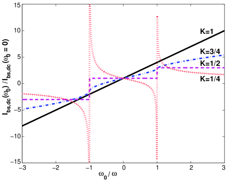
Figure 1: (Color online) DC part of the backscattered current as a function of the bias $\omega_{0}$ for several impurities, when $\omega_{\pm}$ are small. The red (dot), magenta (dash), blue (dash-dot) and black (solid) lines show the results for $K=1/4,1/2,3/4$ and 1 respectively. We have taken $|\sum_{p}U_{p}e^{i(2k_{F}x_{p}+\phi_{p})}|^{2}/|\sum_{p}U_{p}e^{i(2k_{F}x_{p}-\phi_{p})}|^{2}=2:1$.

Figure 1 shows the dc part of the backscattered current as a function of the applied bias, for a fixed non-zero value of the pumping frequency $\omega$, assuming that $\omega$ and $\omega_{0}$ are small. We have used the expression in Eq. (LABEL:idctot) to plot the value of $I_{bs,dc}(\omega_{0})/I_{bs,dc}(\omega_{0}=0)$ as a function of $\omega_{0}/\omega$, for four different values of the parameter $K=1/4,1/2,3/4$ and 1, taking the ratio $|\sum_{p}U_{p}e^{i(2k_{F}x_{p}+\phi_{p})}|^{2}/|\sum_{p}U_{p}e^{i(2k_{F}x_{p}-\phi_{p})}|^{2}=2:1$ as an example. For $K=1/4$, the current diverges at $\omega_{0}=\pm\omega$ as mentioned above. We also note the linear and piecewise constant dependences of the current on $\omega_{0}$ for $K=1$ and 1/2 respectively; this is discussed in Subsec. III. E below.

If we relax the assumptions that $\omega x_{rp}/v$ and $\omega_{0}x_{rp}/v$ are small, then the exact expressions (up to second order in the impurity potentials) for the ac and dc component of the backscattered current are given by

$$I_{bs,dc}^{pr} = \frac{qU_{p}U_{r}\sqrt{\pi}}{4\pi v^{2}\Gamma(K)}\left(\frac{\alpha}{v}\right)^{2K-2}\left(\frac{2|x_{rp}|}{v}\right)^{1/2-K}$$

$$\times [sgn(\omega_{+})~{}|\omega_{+}|^{K-1/2}J_{K-1/2}(|\omega_{+}x_{rp}|/v)$$

$$\times~{}\cos(2k_{F}x_{rp}+\phi_{rp})$$

$$+~{}sgn(\omega_{-})~{}|\omega_{-}|^{K-1/2}~{}J_{K-1/2}(|\omega_{-}x_{rp}|/v)$$

$$\times~{}\cos(2k_{F}x_{rp}-\phi_{rp})],$$

$$I_{bs,ac}^{pr} = \frac{qU_{p}U_{r}\sqrt{\pi}}{4\pi v^{2}\Gamma(K)\cos(\pi K)}\left(\frac{\alpha}{v}\right)^{2K-2}$$ (33)

$$\times \left(\frac{2|x_{rp}|}{v}\right)^{1/2-K}\cos(2k_{F}x_{rp})$$

$$\times [sgn(\omega_{+})~{}|\omega_{+}|^{K-1/2}~{}J_{K-1/2}(|\omega_{+}x_{rp}|/v)$$

$$\times~{}\cos(2\omega t+\phi_{p}+\phi_{r}+sgn(\omega_{+})\pi K)$$

$$+~{}sgn(\omega_{-})~{}|\omega_{-}|^{K-1/2}~{}J_{K-1/2}(|\omega_{-}x_{rp}|/v)$$

$$\times~{}\cos(2\omega t+\phi_{p}+\phi_{r}-sgn(\omega_{-})\pi K)$$

$$+~{}\{|\omega_{+}|^{K-1/2}~{}J_{1/2-K}(|\omega_{+}x_{rp}|/v)$$

$$~{}~{}~{}~{}~{}-~{}|\omega_{-}|^{K-1/2}~{}J_{1/2-K}(|\omega_{-}x_{rp}|/v)\}$$

$$\times~{}\sin(2\omega t+\phi_{p}+\phi_{r})].$$

The Bessel function $J$ is discussed in the Appendix; using a power series expansion given there, we can show that Eqs. (LABEL:idc3-33) reduce to Eqs. (LABEL:idc2-LABEL:iac2) in the limit $\omega_{\pm}x_{rp}/v\to 0$. We note that the expressions in Eqs. (LABEL:idc1-LABEL:iac1) do not change if we relax the assumptions that $\omega$ and $\omega_{0}$ are small.

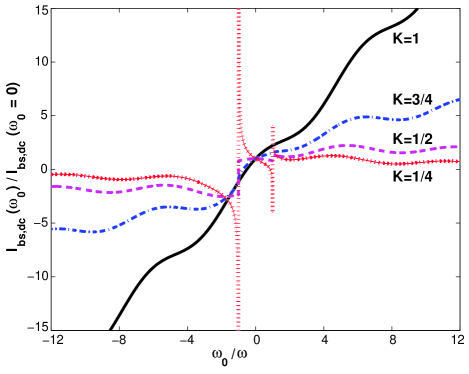
Figure 2: (Color online) DC part of the backscattered current as a function of the bias $\omega_{0}$ for two impurities, when $\omega_{\pm}$ are not small. The red (dot), magenta (dash), blue (dash-dot) and black (solid) lines show the results for $K=1/4,1/2,3/4$ and 1 respectively. We have taken $U_{1}=U_{2}$, $2k_{F}x_{12}=\pi/2$, $\phi_{12}=-\pi/4$, and $\omega x_{12}/v=1$.

Figure 2 shows the dc part of the backscattered current as a function of the applied bias for the case of two impurities, labeled 1 and 2, taking $U_{1}=U_{2}$, $2k_{F}x_{12}=\pi/2$, $\phi_{12}=-\pi/4$, and $\omega x_{12}/v=1$; thus $\omega$ and $\omega_{0}$ are not small, in contrast to the case shown in Fig. 1. We have used the expressions in Eqs. (LABEL:idc1) and (LABEL:idc3) to plot the value of $I_{bs,dc}(\omega_{0})/I_{bs,dc}(\omega_{0}=0)$ as a function of $\omega_{0}/\omega$, for four different values of the parameter $K=1/4,1/2,3/4$ and 1. We see some oscillations in Fig. 2 due to the appearance of the Bessel functions in Eq. (LABEL:idc3). For $K=1/4$, we again see divergences at $\omega_{0}=\pm\omega$.

III.5 $K=1$ and 1/2

We now discuss the special cases $K=1$ and 1/2 where the expressions for some parts of the currents simplify considerably.

For non-interacting fermions with $K=1$, we find from Eqs. (LABEL:idc1-LABEL:iac1) that in the single impurity case,

$$I_{bs,dc}^{pp} = \frac{qU_{p}^{2}}{4\pi v_{F}^{2}}~{}\omega_{0},$$

$$I_{bs,ac}^{pp} = \frac{qU_{p}^{2}}{4\pi v_{F}^{2}}~{}\omega_{0}~{}\cos(2\omega t+2\phi_{p}).$$ (34)

The total current is given by $I=-I_{0}+I_{bs,dc}^{pp}+I_{bs,ac}^{pp}$,

$$I~{}=~{}\frac{q\omega_{0}}{2\pi}~{}\left[-~{}1~{}+~{}\left(\frac{U_{p}\cos(\omega t+\phi_{p})}{v_{F}}\right)^{2}\right].$$ (35)

This is consistent with the fact that the transmission probability across a static point-like barrier of height $U$ is $1-(U/v_{F})^{2}$ up to order $U^{2}$. For the case of several impurities, we find from Eqs. (LABEL:idc2-LABEL:iac2) that

$$I_{bs,dc}^{pr} = \frac{qU_{p}U_{r}}{2\pi v_{F}^{2}}~{}[~{}\omega_{0}~{}\cos(2k_{F}x_{rp})~{}\cos(\phi_{rp}),$$ (36)

$$~{}\quad\quad\quad~{}-~{}\omega~{}\sin(2k_{F}x_{rp})~{}\sin(\phi_{rp})~{}],$$

$$I_{bs,ac}^{pr} = \frac{qU_{p}U_{r}}{2\pi v_{F}^{2}}~{}\omega_{0}~{}\cos(2k_{F}x_{rp})~{}\cos(2\omega t+\phi_{p}+\phi_{r}).$$

Note that the dc part of the current is given by a linear combination of the pure bias part and the pure pumping part, and it agrees with the expression given in Eq. (13).

For $K=1/2$, we can obtain the different parts of the currents by taking the limit $K\to 1/2$ in Eqs. (LABEL:idc1-LABEL:iac1) and (LABEL:idc2-LABEL:iac2). We find that

$$I_{bs,dc}^{pp} = \frac{qU_{p}^{2}}{8\pi\alpha v}~{}[sgn(\omega_{+})~{}+~{}sgn(\omega_{-})],$$

$$I_{bs,dc}^{pr} = \frac{qU_{p}U_{r}}{4\pi\alpha v}[sgn(\omega_{+})\cos(2k_{F}x_{rp}+\phi_{rp})$$

$$\quad\quad\quad~{}+~{}sgn(\omega_{-})\cos(2k_{F}x_{rp}-\phi_{rp})],$$

$$I_{bs,ac}^{pp} = \frac{qU_{p}^{2}}{8\pi\alpha v}[(sgn(\omega_{+})+sgn(\omega_{-}))\cos(2\omega t+2\phi_{p})$$

$$\quad\quad\quad~{}+~{}\frac{2}{\pi}~{}\ln|\frac{\omega_{+}}{\omega_{-}}|~{}\sin(2\omega t+2\phi_{p})],$$

$$I_{bs,ac}^{pr} = \frac{qU_{p}U_{r}}{4\pi\alpha v}[(sgn(\omega_{+})+sgn(\omega_{-}))\cos(2\omega t+\phi_{p}+\phi_{r})$$

$$\quad\quad\quad~{}+~{}\frac{2}{\pi}~{}\ln|\frac{\omega_{+}}{\omega_{-}}|~{}\sin(2\omega t+\phi_{p}+\phi_{r})].$$

Thus the DC parts of the currents do not depend on the precise values of $\omega$ and $\omega_{0}$ if they are unequal, and they have a finite discontinuity when $\omega$ crosses $\pm\omega_{0}$.

To conclude, we see that the dc parts of the currents are linear functions of $\omega_{0},\omega$ for $K=1$, and are piecewise constant functions of $\omega_{0},\omega$ for $K=1/2$.

III.6 Extended impurities

The analysis in Subsec. III. D can be readily generalized to the case where there is an extended region of oscillating potentials makogon2 . Let us replace the discrete set of potentials given in Eq. (3) by an oscillating potential of the following form

$$U(t)~{}=~{}\int dx~{}U(x)\cos[\omega t+\phi(x)]~{}.$$ (39)

We then see from Eq. (LABEL:idctot) that the dc part of the backscattered current is given by

$$I_{bs,dc} = \frac{q}{8\pi v^{2}\Gamma(2K)}\left(\frac{\alpha}{v}\right)^{2K-2}$$

$$\times [sgn(\omega_{+})~{}|\omega_{+}|^{2K-1}|\int dx~{}U(x)~{}e^{i[2k_{F}x+\phi(x)]}|^{2}$$

$$+ sgn(\omega_{-})~{}|\omega_{-}|^{2K-1}|\int dx~{}U(x)~{}e^{i[2k_{F}x-\phi(x)]}|^{2}].$$

to second order in $U(x)$. For the pure pumping case with $\omega_{0}=0$, we find that

$$I_{bs,dc} = -~{}\frac{q}{4\pi v^{2}\Gamma(2K)}\left(\frac{\alpha}{v}\right)^{2K-2}\omega^{2K-1}$$ (41)

$$\times \int\int dxdx^{\prime}~{}U(x)U(x^{\prime})~{}\sin[2k_{F}(x-x^{\prime})]$$

$$\quad\quad~{}\times~{}\sin[\phi(x)-\phi(x^{\prime})].$$

Eq. (41) implies that the charge pumped per cycle, $\Delta Q=(2\pi/\omega)I_{bs,dc}$, scales as $\omega^{2K-2}$; for $K<1$, this grows large in the adiabatic limit $\omega\to 0$. In this limit, we saw earlier that the effective length-dependent impurity strength diverges at small energy scales, which implies that the impurity presents a very large barrier to the electrons and the transmission coefficient is very small. In this limit, it has been argued in Refs. das ; sharma that the pumped charge $\Delta Q$ is quantized to be an integer multiple of $q$.

III.7 Spin-1/2 electrons

For spin-1/2 electrons in one dimension, the phenomenon of spin-charge separation occurs if there are interactions between the electrons. The spin and charge degrees of freedom can be separately bosonized gogolin ; giamarchi . The two bosonic theories are characterized by the parameters $(K_{s},v_{s})$ and $(K_{c},v_{c})$ respectively. For a system with $SU(2)$ rotational invariance, $K_{s}=1$. The ground state expectation value in Eq. (24) then takes the form

$$\langle 0|~{}\psi_{\sigma R}^{\dagger}(x_{p},t^{\prime})\psi_{\sigma L}(x_{p},t^{\prime})\psi_{\sigma L}^{\dagger}(x_{r},t)\psi_{\sigma R}(x_{r},t)~{}|0\rangle$$

$$\sim~{}\frac{1}{[(x_{p}-x_{r})^{2}~{}-~{}(v_{s}(t^{\prime}-t)-i\alpha)^{2}]^{1/2}}$$

$$\quad\times~{}\frac{1}{[(x_{p}-x_{r})^{2}~{}-~{}(v_{c}(t^{\prime}-t)-i\alpha)^{2}]^{K_{c}/2}},$$ (42)

where $\sigma=\uparrow,\downarrow$ is the spin label. The appearance of two different velocities, $v_{s}$ and $v_{c}$, and two different exponents, $1/2$ and $K_{c}/2$, in Eq. (42) makes the expressions for the backscattered current rather complicated. However, we can find the power law of the dependence of the currents on the frequencies by a simple scaling argument. With the approximations made earlier, $\omega x_{rp}/v_{s,c}$ and $\omega_{0}x_{rp}/v_{s,c}\to 0$, we see that the time dependence has changed from $1/(t^{\prime}-t)^{2K}$ in Eq. (24) to $1/(t^{\prime}-t)^{K_{c}+1}$ in Eq. (42). The dependences of the backscattered currents on the frequencies therefore change from $|\omega_{0}\pm\omega|^{2K-1}$ in the spinless case to $|\omega_{0}\pm\omega|^{K_{c}}$ in the spin-1/2 case. Since $K_{c}$ is positive in general, the current no longer diverges as $\omega_{0}\to\pm\omega$.

IV Discussion

We have considered the effects of a bias and a number of weak and harmonically oscillating potentials on charge transport in a Tomonaga-Luttinger liquid. We have computed the backscattered current to second order in the amplitudes of the potentials. For most of our results, we have assumed the oscillation frequency and the bias to be small, but we have relaxed that assumption in Eqs. (LABEL:idc3-33). For our assumption of a Dirac fermion with a linear dispersion to be valid for an experimentally realizable system, we must of course assume that $\omega$ and $\omega_{0}$ are small compared to the band width of the electrons.

We find that the backscattered current is maximized for a traveling potential wave in which the positions and phases of the oscillating potentials are related in a linear way. For spinless electrons, if the interactions are sufficiently repulsive with $K<1/2$, the backscattered current diverges for special values of the bias, namely, for $\omega_{0}\to\pm\omega$. For any repulsive interaction, with $K<1$, the correction to the differential conductance diverges for $\omega_{0}\to\pm\omega$. Finally, we have pointed out a peculiarity which arises when several impurities are present and $K<1/2$; namely, the current must in general be a non-monotonic function of the pumping frequency when there is no bias.

It would be useful to generalize our results to the case of one or more strong impurity potentials, or weak tunnelings between two Tomonaga-Luttinger liquids; the technique of bosonization can be used in such situations also.

Appendix A Some mathematical formulae

We need to evaluate integrals of the form

$$\int_{0}^{\infty}d\tau~{}\frac{\exp(\pm i\Omega\tau)}{((\tau\pm i\alpha)^{2}-x^{2})^{K}},$$ (43)

where $\Omega=\omega_{\pm}$ and $x=x_{rp}/v$. Eq. (43) can be written as the sum of integrals running from $0$ to $x$ and from $x$ to $\infty$. We find that there are several integrals from $0$ to $x$ which cancel each other. One is then left with integrals running from $x$ to $\infty$ in which one can take the limit $\alpha\to 0$ in the denominator. We then use the following results gradshteyn

$$\int_{x}^{\infty}d\tau~{}\frac{\sin(\Omega\tau)}{(\tau^{2}-x^{2})^{K}} = \frac{\sqrt{\pi}}{2}~{}\left(\frac{2x}{\Omega}\right)^{1/2-K}\Gamma(1-K)$$

$$\times~{}J_{K-1/2}(\Omega x),$$

$$\int_{x}^{\infty}d\tau~{}\frac{\cos(\Omega\tau)}{(\tau^{2}-x^{2})^{K}} = -~{}\frac{\sqrt{\pi}}{2}~{}\left(\frac{2x}{\Omega}\right)^{1/2-K}\Gamma(1-K)$$ (44)

$$\times~{}Y_{K-1/2}(\Omega x),$$

where $J$ and $Y$ are Bessel functions of the first and second kind respectively. The above equations are valid for $x,\Omega>0$, and $0<K<1$. We then use the power series expansion abramowitz

$$J_{\nu}(z) = \left(\frac{z}{2}\right)^{\nu}~{}\sum_{n=0}^{\infty}~{}(-1)^{n}\frac{(z/2)^{2n}}{n!~{}\Gamma(n+\nu+1)},$$ (45)

and the relation

$$Y_{\nu}(z) = \frac{1}{\sin{(\pi\nu)}}~{}[\cos(\pi\nu)~{}J_{\nu}(z)~{}-~{}J_{-\nu}(z)]$$ (46)

which is valid for non-integer values of $\nu$.

Finally, the following identities involving Gamma functions are useful abramowitz ,

$$\Gamma(1-z)~{}\Gamma(z) = \frac{\pi}{\sin(\pi z)},$$

$$\Gamma(z)~{}\Gamma(z+1/2) = \frac{\sqrt{\pi}}{2^{2z-1}}~{}\Gamma(2z).$$ (47)

References

- (1)
- (2) S. Datta, Electronic transport in mesoscopic systems (Cambridge University Press, 1995).
- (3) Y. Imry, Introduction to Mesoscopic Physics (Oxford University Press, 1997).
- (4) S. Tarucha, T. Honda, and T. Saku, Sol. St. Comm. 94, 413 (1995).
- (5) C. -T. Liang, M. Pepper, M. Y. Simmons, C. G. Smith, and D. A. Ritchie, Phys. Rev. B 61, 9952 (2000).
- (6) B. E. Kane, G. R. Facer, A. S. Dzurak, N. E. Lumpkin, R. G. Clark, L. N. Pfeiffer, and K. W. West, App. Phys. Lett. 72, 3506 (1998).
- (7) A. Yacoby, H. L. Stormer, N. S. Wingreen, L. N. Pfeiffer, K. W. Baldwin, and K. W. West, Phys. Rev. Lett. 77, 4612 (1996).
- (8) O. M. Auslaender, A. Yacoby, R. de Picciotto, K. W. Baldwin, L. N. Pfeiffer, and K. W. West, Phys. Rev. Lett. 84, 1764 (2000).
- (9) D. J. Reilly, G. R. Facer, A. S. Dzurak, B. E. Kane, R. G. Clark, P. J. Stiles, J. L. O’Brien, N. E. Lumpkin, L. N. Pfeiffer, and K. W. West, Phys. Rev. B 63, 121311(R) (2001).
- (10) C. L. Kane and M. P. A. Fisher, Phys. Rev. B 46, 15233 (1992).
- (11) A. Furusaki and N. Nagaosa, Phys. Rev. B 47, 4631 (1993).
- (12) D. J. Thouless, Phys. Rev. B 27, 6083 (1983).
- (13) Q. Niu, Phys. Rev. Lett. 64, 1812 (1990).
- (14) M. Büttiker, H. Thomas, and A. Prêtre, Z. Phys. B 94, 133 (1994).
- (15) P. W. Brouwer, Phys. Rev. B 58, R10135 (1998).
- (16) P. W. Brouwer, Phys. Rev. B 63, 121303(R) (2001).
- (17) I. L. Aleiner and A. V. Andreev, Phys. Rev. Lett. 81, 1286 (1998).
- (18) J. E. Avron, A. Elgart, G. M. Graf, and L. Sadun, Phys. Rev. Lett. 87, 236601 (2001); Phys. Rev. B 62, R10618 (2000); J. Stat. Phys. 116, 425 (2004).
- (19) O. Entin-Wohlman, A. Aharony and Y. Levinson, Phys. Rev. B 65, 195411 (2002).
- (20) O. Entin-Wohlman and A. Aharony, Phys. Rev. B 66, 035329 (2002).
- (21) Y. M. Galperin, O. Entin-Wohlman, and Y. Levinson, Phys. Rev. B 63, 153309 (2001).
- (22) A. Aharony and O. Entin-Wohlman, Phys. Rev. B 65, 241401(R) (2002).
- (23) V. Kashcheyevs, A. Aharony, and O. Entin-Wohlman, Phys. Rev. B 69, 195301 (2004), and Eur. Phys. J. B 39, 385 (2004).
- (24) M. Moskalets and M. Büttiker, Phys. Rev. B 66, 205320 (2002), and Phys. Rev. B 68, 075303 (2003).
- (25) S. W. Kim, Phys. Rev. B 66, 235304 (2002).
- (26) B. Wang, J. Wang, and H. Guo, Phys. Rev. B 68, 155326 (2003), and Phys. Rev. B 65, 073306 (2002).
- (27) L. Arrachea, Phys. Rev. B 72, 125349 (2005), and Phys. Rev. B 72, 121306(R) (2005).
- (28) L. E. F. Foa Torres, Phys. Rev. B 72, 245339 (2005).
- (29) L. Arrachea, C. Naon, and M Salvay, arXiv:0704.2329.
- (30) A. Banerjee, S. Das, and S. Rao, cond-mat/0307324.
- (31) S. Banerjee, A. Mukherjee, S. Rao, and A. Saha, cond-mat/0608267.
- (32) G. R. Aizin, G. Gumbs, and M. Pepper, Phys. Rev. B 58, 10589 (1998); G. Gumbs, G. R. Aizin, and M. Pepper, Phys. Rev. B 60, R13954 (1999).
- (33) K. Flensberg, Q. Niu, and M. Pustilnik, Phys. Rev. B 60, R16291 (1999).
- (34) P. A. Maksym, Phys. Rev. B 61, 4727 (2000).
- (35) A. M. Robinson and C. H. W. Barnes, Phys. Rev. B 63, 165418 (2001).
- (36) M. M. Mahmoodian, L. S. Braginsky, and M. V. Entin, Phys. Rev. B 74, 125317 (2006).
- (37) M. Strass, P. Hänggi, and S. Kohler, Phys. Rev. Lett. 95, 130601 (2005).
- (38) S. Kohler, J. Lehmann, and P. Hänggi, Phys. Rep. 406, 379 (2005).
- (39) A. Agarwal and D. Sen, J. Phys. Condens. Matter 19, 046205 (2007).
- (40) M. Switkes, C. M. Markus, K. Campman, and A. C. Gossard, Science 283, 1905 (1999).
- (41) V. I. Talyanskii, J. M. Shilton, M. Pepper, C. G. Smith, C. J. B. Ford, E. H. Linfield, D. A. Ritchie, and G. A. C. Jones, Phys. Rev. B 56, 15180 (1997).
- (42) J. Cunningham, V. I. Talyanskii, J. M. Shilton, M. Pepper, M. Y. Simmons, and D. A. Ritchie, Phys. Rev. B 60, 4850 (1999); J. Cunningham, V. I. Talyanskii, J. M. Shilton, M. Pepper, A. Kristensen, and P. E. Lindelof, Phys. Rev. B 62, 1564 (2000).
- (43) V. I. Talyanskii, D. S. Novikov, B. D. Simons, and L. S. Levitov, Phys. Rev. Lett. 87, 276802 (2001).
- (44) P. J. Leek, M. R. Buitelaar, V. I. Talyanskii, C. G. Smith, D. Anderson, G. A. C. Jones, J. Wei, and D. H. Cobden, Phys. Rev. Lett. 95, 256802 (2005).
- (45) S. Das and S. Rao, Phys. Rev. B 71, 165333 (2005).
- (46) C. de C. Chamon, D. E. Freed, and X. G. Wen, Phys. Rev. B 51, 2363 (1995) and Phys. Rev. B 53, 4033 (1996).
- (47) C. de C. Chamon, D. E. Freed, S. A. Kivelson, S. L. Sondhi, and X. G. Wen, Phys. Rev. B 55, 2331 (1997).
- (48) P. Sharma and C. Chamon, Phys. Rev. B 68, 035321 (2003), and Phys. Rev. Lett. 87, 096401 (2001).
- (49) D. E. Feldman and Y. Gefen, Phys. Rev. B 67, 115337 (2003).
- (50) D. Makogon, V. Juricic, and C. Morais Smith, Phys. Rev. B 74, 165334 (2006).
- (51) D. Makogon, V. Juricic, and C. Morais Smith, cond-mat/0609372.
- (52) D. Schmeltzer, Phys. Rev. B 63, 125332 (2001).
- (53) D. E. Feldman, S. Scheidl, and V. M. Vinokur, Phys. Rev. Lett. 94, 186809 (2005).
- (54) F. Cheng, and G. Zhou, Phys. Rev. B 73, 125335 (2006).
- (55) B. Braunecker and D. E. Feldman, cond-mat/0610847.
- (56) T. L. Schmidt and A. Komnik, cond-mat/0702312.
- (57) A. O. Gogolin, A. A. Nersesyan, and A. M. Tsvelik, Bosonization and Strongly Correlated Systems (Cambridge University Press, Cambridge, 1998).
- (58) S. Rao and D. Sen, in Field Theories in Condensed Matter Physics, edited by S. Rao (Hindustan Book Agency, New Delhi, 2001).
- (59) T. Giamarchi, Quantum Physics in One Dimension (Oxford University Press, Oxford, 2004).
- (60) I. S. Gradshteyn and I. M. Ryzhik, Table of Integrals, Series, and Products (Academic Press, London, 2000).
- (61) M. Abramowitz and I. A. Stegun, Handbook of Mathematical Functions (Dover Publications, New York, 1972).