Mass flows and angular momentum density for $p_{x}+ip_{y}$ paired fermions in a harmonic trap

Abstract

We present a simple two-dimensional model of a $p_{x}+ip_{y}$ superfluid in which the mass flow that gives rise to the intrinsic angular momentum is easily calculated by numerical diagonalization of the Bogoliubov-de Gennes operator. We find that, at zero temperature and for constant director $\bf l$, the mass flow closely follows the Ishikawa-Mermin-Muzikar formula ${\bf j}_{\rm mass}={1\over 2}{\rm curl\/}(\rho\hbar{\bf l}/2)$.

I Introduction

Controversies over the “instrinsic angular momentum” of the A phase of superfluid ³He have a long history [1, 2], but the issue has contemporary relevance for the search for boundary currents in the suspected $p_{x}+ip_{y}$ superconducting phase of Sr₂RuO₄ [3], and for experiments on possible $p$-wave versions of atomic Fermi condensates [4].

Behind the competing computations of the ground-state angular momentum density lie two competing intuitive pictures. In the first the superfluid is regarded as a Bose condensate of Cooper pairs, each pair possessing angular momentum $\hbar$. In this picture, and at temperature $T=0$, the total angular momentum of a spatially uniform system of ${\mathcal{N}}$ particles should be ${1\over 2}{\mathcal{N}}\hbar$. The second picture begins with the observation that in the BCS regime, where $\Delta\ll\epsilon_{F}$, the opening of the energy gap $\Delta$ affects only states lying within an energy range of a few $\Delta$ about the Fermi surface at $E=\epsilon_{F}$. It is therefore anticipated that the “naïve” estimate of ${1\over 2}{\mathcal{N}}\hbar$ will be reduced by a factor of $\Delta/\epsilon_{F}$ [5], or even by a factor of $(\Delta/\epsilon_{F})^{2}$ [6].

For a system consisting of a fixed (even) number of particles with a common, angular momentum $l_{z}=1$ pair wavefunction $\psi({\bf r}_{1},{\bf r}_{2})$, the antisymmetric many-body wavefunction is given by the pfaffian ${\rm Pf}[\psi({\bf r}_{i},{\bf r}_{j})]$, and is undoubtedly an eigenstate of the angular momentum operator $L_{z}$ with eigenvalue ${1\over 2}\hbar{\mathcal{N}}$ [7]. The problem is that $\psi({\bf r}_{1},{\bf r}_{2})$ is usually computed for a spatially uniform system, and a uniform system is not suitable for computing angular momentum: a substantial contribution to the angular momentum can arise from a small current at large distances—in particular near the walls of the container, where the density abruptly drops to zero.

Once we allow spatial variations of the fluid density or order parameter, analytic expressions can only be obtained by approximate methods. Unfortunately, different approaches have led to different answers (see ref. [1] for a brief summary). The Gorkov gradient expansion, for example, computes Green functions for the Bogoliubov-de Gennes (BdG) equation, and in this formalism the angular momentum arises from the spectral asymmetry of the BdG differential operator. This asymmetry is closely related to the phenomenon of topologically induced fractional charge, and to the axial anomaly of QED. Now the axial anomaly is quite a subtle phenomenon and can easily be missed if one makes naïve manipulations in conditionally convergent integrals, or appeals to symmetries that are vitiated by boundary conditions. We claim however, that when solved exactly, the BdG equation produces results entirely consistent with the Cooper-pair wave function approach: there is no $\Delta/\epsilon_{F}$ suppression, and the ground-state intrinsic angular momentum is ${1\over 2}\hbar$ per particle.

In this paper we use the BdG equation to obtain numerical results for the angular momentum and associated mass-flows in a two-dimensional model of $p_{x}+ip_{y}$ superfluid fermions confined in a harmonic trap. Numerical computations of the angular momentum in a cylindrical container have been obtained by Kita [8], and our results are entirely consistent with this earlier work. We believe, however, that the simplicity of the present model, where the phenomena can be studied interactively with a few lines of Mathematica^TM code, make it of interest. We begin in sections II and III with a brief review of the Bogoliubov de Gennes formalism and the two-dimensional Harmonic oscillator. In section IV we show how symmetries and the harmonic oscillator selection rules serve to reduce the BdG equation to a tridiagonal matrix eigenvalue problem which is solved numerically in section V. We end in section VI with a brief discussion of what we conjecture to be the origin of the much smaller angular momentum found by some older methods.

II Superfluidity and the Bogoliubov-de Gennes equation

Because of the history of controversy in this subject, it is essential that we explain exactly how we do our calculations. We begin, therefore, with a brief review of the Bogoliubov-de Gennes formalism.

Suppose that $H_{ij}$ is an $N$-by-$N$ matrix representing a one-particle (i.e. first quantized) Hamiltonian $H$. The second-quantized many-body hamiltonian corresponding to this is

$${\hat{H}}=\hat{a}^{\dagger}_{i}H_{ij}\hat{a}_{j},$$ (1)

where a sum over the repeated indices is to be understood. Here $\hat{a}^{\dagger}_{i}$ and $\hat{a}_{i}$ are second-quantization fermion creation and annihilation operators obeying

$$\{\hat{a}_{i},\hat{a}_{j}\}=\{\hat{a}^{\dagger}_{i},\hat{a}^{\dagger}_{j}\}=0,\quad\{\hat{a}_{i},\hat{a}^{\dagger}_{j}\}=\delta_{ij}.$$ (2)

The operator $\hat{a}^{\dagger}_{i}$ creates a particle in state $i$ and $\hat{a}_{i}$ destroys such a particle. If we represent $H$ in a continuous basis, the index “$i$” should be understood to incorporate both the space co-ordinate $x$, and any spin index. A sum over $i$ therefore implies both an integral over real space and a sum over spin components.

To account for the effect of a condensate of Cooper pairs, we allow pairs of particles to disappear into or appear out of the background, and the second-quantized $\hat{H}$ is replaced by the Bogoliubov Hamiltonian

$$\hat{H}_{\rm Bogoliubov}=\hat{a}^{\dagger}_{i}H_{ij}\hat{a}_{j}+{\textstyle{1\over 2}}\Delta_{ij}\hat{a}^{\dagger}_{i}\hat{a}^{\dagger}_{j}+{\textstyle{1\over 2}}\Delta^{\dagger}_{ij}\hat{a}_{i}\hat{a}_{j}.$$ (3)

The gap-function matrix $\Delta_{ij}$ is skew symmetric. Different forms of $\Delta_{ij}$ describe different condensates and result in different patterns of symmetry breaking. The entries in $\Delta_{ij}$ are usually determined by a self consistency condition, or gap equation. In the present work we are more concerned with the consequences of a non-zero $\Delta_{ij}$ than with its origin, and so will take its magnitude and form as something imposed externally.

We can write the particle-number non-conserving Bogoliubov Hamiltonian as

$$\hat{H}_{\rm Bogoliubov}={1\over 2}\left(\matrix{\hat{a}^{\dagger}_{i}&\hat{a}_{i}}\right)\left(\matrix{H_{ij}&\phantom{-}\Delta_{ij}\cr\Delta^{\dagger}_{ij}&-H^{T}_{ij}}\right)\left(\matrix{\hat{a}_{j}\cr\hat{a}^{\dagger}_{j}}\right)+{1\over 2}{\rm tr\,}H,$$ (4)

where $H^{T}$ denotes the transpose of the hermitian matrix $H$. The two-by-two block-matrix form of the many-body Hamiltonian conveniently allows it to be diagonalized by means of a Bogoliubov transformation. We first solve the single-particle Bogoliubov-de-Gennes (BdG) eigenvalue problem

$$\left(\matrix{H&\Delta\cr\Delta^{\dagger}&-H^{T}}\right)\left(\matrix{\vec{u}_{m}\cr\vec{v}_{m}}\right)=E_{m}\left(\matrix{\vec{u}_{m}\cr\vec{v}_{m}}\right).$$ (5)

Here $\vec{u}_{m}$ and $\vec{v}_{m}$ are $N$-dimensional column vectors, which we take to be normalized so that $|\vec{u}_{m}|^{2}+|\vec{v}_{m}|^{2}=1$. If we explicitly display the column-vector index $i$, these vectors can be regarded as $N$-by-$N$ matrices with entries $u_{im}$ and $v_{im}$. Taking the complex conjugate of (5) tells us that

$$\left(\matrix{H&\Delta\cr\Delta^{\dagger}&-H^{T}}\right)\left(\matrix{\vec{v}^{*}_{m}\cr\vec{u}^{*}_{m}}\right)=-E_{m}\left(\matrix{\vec{v}^{*}_{m}\cr\vec{u}^{*}_{m}}\right),$$ (6)

and so the BdG-operator eigenvalues come in $\pm$ pairs. We will always use the symbol $E_{m}$ to refer to the positive eigenvalue, and a sum over $N$ otherwise unspecified eigenvectors is a sum over the positive $E_{m}$ eigenvectors. The manner in which the BdG operator doubles the spectrum, and how we retain only the positive part, is illustrated in Figure 1.

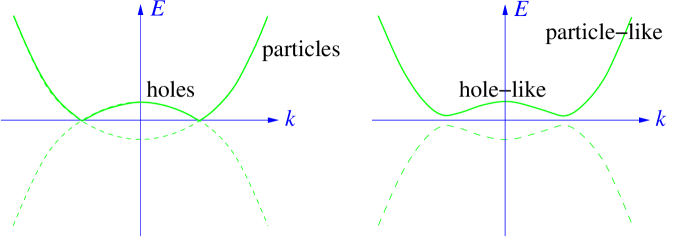
Figure 1: The BdG operator spectrum for a one-dimensional non-relativistic gas with $E(k)=k^{2}/2-\mu$. Left: the spectrum with $\Delta=0$. Right: the spectrum after a gap is opened by a non-zero $\Delta$. In each case the part of the spectrum with BdG eigenvalue $E>0$ is shown as a solid line, and the part with $E<0$ is shown dashed. For $\Delta\neq 0$, the $E>0$ “particle-like” region has $|\vec{v}|\approx 0$ and $|\vec{u}|\approx 1$, and the “hole-like” region has $|\vec{u}|\approx 0$ and $|\vec{v}|\approx 1$.

We now set

$$\hat{a}_{i} = u_{im}\hat{b}_{m}+v^{*}_{im}\hat{b}^{\dagger}_{m}$$

$$\hat{a}^{\dagger}_{i} = v_{im}\hat{b}_{m}+u^{*}_{im}\hat{b}^{\dagger}_{m}.$$ (7)

The mutual orthonormality and completeness of the eigenvectors $(\vec{u}_{m},\vec{v}_{m})^{T}$ ensures that the $\hat{b}_{m}$, $\hat{b}^{\dagger}_{m}$ have the same anti-commutation relations as the $\hat{a}_{i}$, $\hat{a}^{\dagger}_{i}$. In terms of the $\hat{b}_{m}$, $\hat{b}^{\dagger}_{m}$, the second-quantized Hamiltonian becomes

$$\hat{H}_{\rm Bogoliubov}=\sum_{m=1}^{N}E_{m}\hat{b}^{\dagger}_{m}\hat{b}_{m}-{1\over 2}\sum_{m=1}^{N}E_{m}+{1\over 2}\sum_{i=1}^{N}E^{(0)}_{i}.$$ (8)

Here the $E^{(0)}_{i}$ are the eigenvalues of $H_{ij}$. Unlike the $E_{m}$, these can be of either sign. If all the quasi-particle excitation energies $E_{m}$ are strictly positive, the new ground state is non degenerate and is the unique state ${|0\rangle}_{b}$ annihilated by all the $\hat{b}_{m}$. The ground-state expectation value of an operator $\hat{O}=\hat{a}^{\dagger}_{i}O_{ij}\hat{a}_{j}$ is therefore

$${\langle\hat{O}\rangle} = {}_{b}{\langle 0|}\hat{a}^{\dagger}_{i}O_{ij}\hat{a}_{j}{|0\rangle}_{b}$$ (9)

$$= {}_{b}{\langle 0|(v_{im}\hat{b}_{m}+u^{*}_{im}\hat{b}^{\dagger}_{m})O_{ij}(u_{jn}\hat{b}_{n}+v^{*}_{jn}\hat{b}^{\dagger}_{n})|0\rangle}_{b}$$

$$= v_{im}O_{ij}v^{*}_{jm}$$

$$= \sum_{m=1}^{N}\vec{v}_{m}^{T}O\vec{v}^{*}_{m}.$$

Because of the $E\leftrightarrow-E$, $\vec{u}\leftrightarrow\vec{v}^{*}$ symmetry, we could equivalently write this last expression as $\sum\vec{u}_{m}^{\dagger}O\vec{u}_{m}$, the sum being taken over the $N$ negative-energy eigenstates of ${\hat{H}}_{\rm Bogoliubov}$, which we think of as being a filled Dirac sea.

For example, the average number of particles present in the system is found by taking $O_{ij}=\delta_{ij}$, and is

$${\mathcal{N}}={{}_{b}}{\langle 0|}{\hat{a}^{\dagger}_{i}\hat{a}_{i}}{|0\rangle}_{b}=v_{im}v^{*}_{im}=\sum_{m=1}^{N}|\vec{v}_{m}|^{2}=\sum_{{\rm negative}\,E}|\vec{u}_{m}|^{2}.$$ (10)

When $\Delta\equiv 0$, this sum will be equal to the number of negative-energy eigenstates of $H_{ij}$.

Although we will not make use of it, it is worth pointing out that if we define the matrix

$$\psi_{ij}=v^{*}_{im}(u^{-1})^{*}_{mj},$$ (11)

then then the orthogonality and completeness conditions tell us that $\psi_{ij}=-\psi_{ji}$. The new ground-state ${|0\rangle}_{b}$ can be written in terms of $\psi_{ij}$ as

$${|0\rangle}_{b}=C\exp\left\{{\textstyle{1\over 2}}\hat{a}^{\dagger}_{i}\hat{a}^{\dagger}_{j}\psi_{ij}\right\}{|0\rangle}_{a}.$$ (12)

Here ${|0\rangle}_{a}$ is the vacuum state annihilated by all the $\hat{a}_{i}$, and $C$ is a normalization constant. This result exhibits the ground state as a coherent superposition of paired states, with $\psi_{ij}$ being the un-normalized Cooper-pair wavefunction. The state ${|0\rangle}_{b}$ gives a non-zero expectation value for the fermion-number non-conserving order parameter

$${}_{b}{\langle 0|}{\hat{a}_{i}\hat{a}_{j}}{|0\rangle}_{b}=\sum_{n}u_{in}v^{*}_{jn},$$ (13)

and so possesses a sharp order-parameter phase and an uncertain particle number. If we desire to work with a fixed (even) number of particles ${\mathcal{N}}$, we should retain only the ${1\over 2}{\mathcal{N}}$-th term in the series expansion of the exponential in equation (12). The resulting many-body wavefunction is then the pfaffian

$$\Psi(i_{1},\ldots,i_{{\mathcal{N}}})\stackrel{{\scriptstyle\rm def}}{{=}}{}_{a}{\langle 0|}{\hat{a}_{i_{1}}\cdots\hat{a}_{i_{\mathcal{N}}}}{|{\mathcal{N}}\rangle}={\rm Pf}[\psi_{i_{\alpha},i_{\beta}}].$$ (14)

In the large $\mathcal{N}$ limit there should be no locally measurable physical distinction between the sharp-phase and the sharp-particle-number ground states.

III Two-dimensional Harmonic oscillator

We consider a model that consists of spinless fermions confined in a harmonic trap in the $x$-$y$ plane. The one-particle Hamiltonian $H$ of section II is therefore that of the two-dimensional harmonic oscillator:

$$H={1\over 2}\left(p_{x}^{2}+p_{y}^{2}+\omega^{2}(x^{2}+y^{2})\right).$$ (15)

Here, for example, $p_{x}=-i\hbar\partial/\partial x$ and so $[x,p_{x}]=i\hbar$. We have taken the mass of the trapped particles to be unity. We define the usual harmonic-oscillator ladder operators

$$a_{x}=\sqrt{{\omega\over 2\hbar}}\left(x+i{p_{x}\over\omega}\right),\quad a_{x}^{\dagger}=\sqrt{{\omega\over 2\hbar}}\left(x-i{p_{x}\over\omega}\right),$$ (16)

and similarly $a_{y}$ and $a^{\dagger}_{y}$. These operators obey

$$[a_{x},a^{\dagger}_{x}]=[a_{y},a^{\dagger}_{y}]=1,\quad[a_{x},a_{y}]=[a^{\dagger}_{x},a_{y}]=0,$$ (17)

and, in terms of them,

$$H=\hbar\omega(a_{x}^{\dagger}a_{x}+a_{y}^{\dagger}a_{y}+1).$$ (18)

The normalized eigenstates can be written as

$${|n_{x},n_{y}\rangle}={(a^{\dagger}_{x})^{n_{x}}\over\sqrt{n_{x}!}}{(a^{\dagger}_{y})^{n_{y}}\over\sqrt{n_{y}!}}{|0,0\rangle},$$ (19)

and have energy eigenvalues $E_{n_{x},n_{y}}=\hbar\omega(n_{x}+n_{y}+1)$.

We will find it more useful to work in a basis in which the angular momentum operator

$$L_{z}\equiv xp_{y}-yp_{x}=ih(a^{\dagger}_{y}a_{x}-a^{\dagger}_{x}a_{y})$$ (20)

is diagonal with eigenvalues $\hbar l$. To construct this basis, we define new ladder operators

$$b_{1}^{\dagger}={1\over\sqrt{2}}(a_{x}^{\dagger}+ia_{y}^{\dagger}),\quad b_{2}^{\dagger}={1\over\sqrt{2}}(a_{x}^{\dagger}-ia_{y}^{\dagger}),$$ (21)

which obey

$$[L_{z},b_{1}^{\dagger}]=\hbar b_{1}^{\dagger},\quad[L_{z},b_{2}^{\dagger}]=-\hbar b_{2}^{\dagger}.$$ (22)

Consequently $b^{\dagger}_{1}$ increases the angular momentum quantum number $l$ by unity and $b^{\dagger}_{2}$ decreases it by unity. It terms of these new operators we have

$$H=\hbar\omega(b^{\dagger}_{1}b_{1}+b_{2}^{\dagger}b_{2}+1),$$ (23)

and the eigenstates become

$${|n,l\rangle}={(b_{1}^{\dagger})^{N}\over\sqrt{N!}}{(b_{2}^{\dagger})^{M}\over\sqrt{M!}}{|0,0\rangle},\quad n=N+M,\quad l=N-M.$$ (24)

The angular momentum of the state ${|n,l\rangle}$ is $\hbar l$ and its energy is $E_{n,l}=\hbar\omega(n+1).$ The set of states with energy quantum number $n$ is $(n+1)$-fold degenerate, the angular-momentum quantum number $l$ running from $l=-n$ to $l=n$ in steps of two. (See Figure 2.)

We will require the normalized real-space wavefunctions ${\langle r,\theta|n,l\rangle}$ corresponding to these eigenstates. These wavefunctions are commonly written as

$$\psi_{N,l}(r,\theta)\equiv{\langle r,\theta|2N+|l|,l\rangle}=\omega^{|l|+1/2}\sqrt{{N!\over\pi(N+|l|)!}}e^{il\theta}r^{l}e^{-\omega r^{2}/2}L^{|l|}_{N}(\omega r^{2}),$$ (25)

where $L^{|m|}_{n}(x)$ is the associated Legendre polynomial

$$L^{|m|}_{n}(x)={x^{-|m|}e^{x}\over n!}{d^{n}\over dx^{n}}e^{-x}x^{n+|m|},$$ (26)

which is of degree $n$. As the notation ${\langle r,\theta|2N+|l|,l\rangle}$ indicates, these states have energy

$$E_{N,l}=\hbar\omega(2N+|l|+1),$$ (27)

and so the integer $N$ counts the height (starting from zero at the lowest point) of the state in the column of eigenstates of angular momentum $l$.

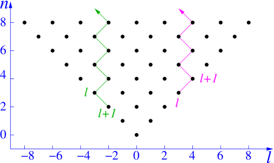
Figure 2: The low-lying part of the harmonic oscillator spectrum. The zig-zag paths indicate how states are coupled by the tridiagonal matrix $H^{(l)}$. For $l$ positive, the first entry in the eigenvector will be a “$v$”, and the second entry a “$u$,” and so on. For $l$ negative, the $u$’s and $v$’s are interchanged.

IV Bogoliubov-de Gennes eigenstates

We now suppose that some suitable interaction has caused our fermions to enter a superfluid phase characterized by an order parameter with $p_{x}+ip_{y}$ symmetry. We can think of the fluid as being a single atomic layer of ³He in the A-phase and with the angular momentum director $\bf l$ of the Cooper pairs pointing in the $+\hat{z}$ direction. We therefore wish to diagonalize the Bogoliubov-de Gennes operator

$$H_{\rm BdG}=\left(\matrix{H-\mu&\Delta(p_{x}+ip_{y})\cr\Delta(p_{x}-ip_{y})&-(H-\mu)}\right).$$ (28)

Here $H$ is the harmonic oscillator hamiltonian, $\mu$ is a chemical potential that controls the number of particles in the trap, and $\Delta$ is a scalar parameter. The off-diagonal term

$$\Delta(p_{x}+ip_{y})=i\Delta\sqrt{\hbar\omega}(b_{1}^{\dagger}-b_{2})$$ (29)

increases the angular momentum quantum number of any state on which it acts by unity, and represents the effect of the condensate of Cooper pairs, each pair possessing angular momentum $+\hbar\hat{z}$.

The eigenstates with eigenvalue $E=E_{m,l}$ will be of the form

$$\Psi_{m,l}(r,\theta)=\left[\matrix{iu_{m,l}(r,\theta)\cr v_{m,l}(r,\theta)}\right]=\left[\matrix{i\sum_{n}u_{m,l}^{n}{\langle r,\theta|n,l+1\rangle}\cr\sum_{n}v_{m,l}^{n}{\langle r,\theta|n,l\rangle}}\right].$$ (30)

The sum over $n$ is over all harmonic-oscillator states consistent with the $l$ quantum number. The pair $(n,l)$ corresponds to the index “$i$” in the general theory in section II. We choose to label the BdG eigenstates by the angular momentum of the lower component “$v$.” Because of the unit off-set between the angular momentum of the $u$’s and $v$’s, the $E\leftrightarrow-E$ pairing is between eigenstates states with angular-momentum label $l$ and those with label $-l-1$.

In the harmonic-oscillator eigenstate basis, and for any fixed $l$, the BdG operator reduces to a tridiagonal matrix connecting only the $l$ and $l+1$ subspaces. The pattern of $H_{\rm BdG}$-connected states is shown in Figure 2 for both positive and negative $l$. This pattern depends on the sign of $l$ because, for $l$ is negative, the ladder operator $b_{2}$ appearing in $p_{x}+ip_{y}$ acts non-trivially on ${||l|,-|l|\rangle}$ to yield a state with lower energy. When $l$ is positive, however, it annihilates ${|l,l\rangle}$. The factor of $i$ in the upper entry of the column vector $\Psi_{m,l}$ has been inserted to eliminate $i$’s and minus signs in the tridiagonal matrix, so that it becomes a real symmetric matrix with positive off-diagonal terms.

The necessary matrix elements can be read-off from

$$i(b^{\dagger}_{1}-b_{2}){|n,l\rangle} = i\sqrt{{n+l+2\over 2}}{|n+1,l+1\rangle}-i\sqrt{{n-l\over 2}}{|n-1,l+1\rangle}$$

$$i(b^{\dagger}_{2}-b_{1}){|n,l+1\rangle} = i\sqrt{{n-l-1\over 2}}{|n+1,l\rangle}-i\sqrt{{n+l+1\over 2}}{|n-1,l\rangle}$$

$$(H-\mu){|n,l\rangle} = \epsilon_{n}{|n,l\rangle},$$ (31)

where

$$\epsilon_{n}=\hbar\omega(n+1)-\mu.$$

For $l$ positive or zero, and with $h\omega=1$, the $(l,l+1)$-subspace BdG matrix takes the form,

$$H^{(l)}=\left[\matrix{-\epsilon_{l}&\Delta\sqrt{l+1}&&&&&\cr\Delta\sqrt{l+1}&\epsilon_{l+1}&\Delta\sqrt{1}&&&&\cr&\Delta\sqrt{1}&-\epsilon_{l+2}&\Delta\sqrt{l+2}&&&\cr&&\Delta\sqrt{l+2}&\epsilon_{l+3}&\Delta\sqrt{2}&\cr&&&\Delta\sqrt{2}&-\epsilon_{l+4}&\ddots\cr&&&&\ddots&\ddots\cr}\right].$$ (32)

All entries more than one step away from the diagonal are zero. When $l$ is strictly negative the $(-|l|,-|l|+1)$-subspace BdG matrix becomes

$$H^{(l)}=\left[\matrix{\epsilon_{-l-1}&\Delta\sqrt{-l}&&&&&\cr\Delta\sqrt{-l}&-\epsilon_{-l}&\Delta\sqrt{1}&&&&\cr&\Delta\sqrt{1}&\epsilon_{-l+1}&\Delta\sqrt{-l+1}&&&\cr&&\Delta\sqrt{-l+1}&-\epsilon_{-l+2}&\Delta\sqrt{2}&\cr&&&\Delta\sqrt{2}&\epsilon_{-l+3}&\ddots\cr&&&&\ddots&\ddots\cr}\right].$$ (33)

In either case, the $i,j$-th matrix element links states with $i$,$j$ labeling the distance from the lowest point along the zig-zag paths shown in Figure 1. The entries in the $m$-th eigenvector of $H^{(l)}$ will therefore consist of alternating $u_{m,l}^{n}$’s and $v_{m,l}^{n}$’s, the first entry being a “$v$” when $l$ is positive, and a “$u$” when $l$ is negative.

It is an easy task to numerically diagonalize a tridiagonal matrix, and so the effect of the gap parameter $\Delta$ on the spectrum can be explored.

V Numerical Results

We have computed [9] the spectrum and the eigenvectors $u_{m,l}^{n}$ and $v_{m,l}^{n}$ for a variety of values of $\mu$ and $\Delta$. Typical results are displayed in this section. In all these plots we have set $\hbar\omega$ to unity. Changing the value of $\omega$ serves only to rescale the energy and $r$.

Figure 3: Part of the BdG operator eigenvalue spectrum for $\mu=40.1$ and $\Delta=0.5$. We have suppressed the axes for clarity. The horizontal co-ordinate, the angular momentum eigenvalue $l$, runs from $-55$ to $+55$, and the eigenvalues $E_{m,l}$ are plotted vertically. Each column of eigenvalues is the result of diagonalizing a 100-by-100 tridiagonal matrix.

Figure 3 shows a plot of the eigenvalues for the case $\mu=40.1$ and $\Delta=0.5$. The interpenetrating wedges of $\pm E$ copies of the harmonic oscillator spectrum are clearly visible, as is the gap lying symmetrically about about $\epsilon=0$. The family of states crossing the gap from the upper “continuum” to the lower as $l$ increases is a chiral Majorana edge mode whose existence was first pointed out by Volovik [10], and whose importance for the analogy with the Pfaffian quantum Hall state was stressed by Read and Green [11].

Figure 4: Fluid density $\rho(r)$ as a function of radius for the case $\mu=40.1$, $\Delta=0.5$. The number of particles in the fluid is ${\mathcal{N}}=2\pi\int_{0}^{\infty}\rho(r)\,rdr=840$.

We also show a plot (Figure 4) of the fluid density

$$\rho(r)=\sum_{l,m}|v_{m,l}(r,\theta)|^{2}$$ (34)

as a function of radius $r$. The $\Delta=0.5$ density profile differs from that for $\Delta=0$ only by being slightly smoother. It closely follows the Thomas-Fermi density

$$\rho_{\rm TF}(r)=\cases{{1\over 2\pi}\left(\mu-{1\over 2}r^{2}\right),&$r<\sqrt{2\mu},$\cr 0,&$r>\sqrt{2\mu}.$}$$ (35)

The Thomas-Fermi approximation estimates the particle number to be

$${\mathcal{N}}_{\rm TF}=2\pi\int_{0}^{\sqrt{2\mu}}\rho_{\rm TF}(r)\,rdr={1\over 2}\mu^{2}.$$ (36)

The actual particle number for the free-particle case $\Delta=0$ is given by ${\mathcal{N}}_{0}={1\over 2}\lfloor\mu\rfloor(\lfloor\mu\rfloor+1)$, where $\lfloor\mu\rfloor$ indicates the integer part of $\mu$. When $\Delta$ becomes non-zero the particle-hole asymmetry in the harmonic oscillator density of states causes the particle number at fixed $\mu$ to creep upwards. The effect is small for small $\Delta$, however.

Figure 5: Angular momentum density $L(r)$ for the same parameters as Figure 4. The total angular momentum is $L_{\rm tot}=2\pi\int_{0}^{\infty}L(r)\,rdr=410$. Thus, for these parameters, $L_{\rm tot}/{\mathcal{N}}=0.49$.

Figure 6: The ground state angular momentum per particle $L_{\rm tot}/{\mathcal{N}}$ plotted as a function of $\Delta$ for $\mu=40.1$. The discontinuous steps in the rising part of the graph are due to individual levels crossing $\epsilon=0$, and so changing their occupation. The $\Delta>0.05$ ground state is therefore not adiabatically connected to the $\Delta=0$ ground state.

Figure 5 plots the ground state angular momentum density

$$L(r)={\langle\hat{L}_{z}\rangle}=\sum_{l,m}v_{m,l}\left(-i{\partial\over\partial\theta}\right)v^{*}_{m,l}=-\sum_{l,m}l|v_{m,l}(r,\theta)|^{2}$$ (37)

as a function of $r$ for the same parameters, and Figure 6 shows the angular momentum per particle as a function of $\Delta$. Except for very small $\Delta$ we find that

$$L_{\rm tot}=2\pi\int_{0}^{\infty}L(r)\,rdr\approx{1\over 2}{\mathcal{N}}.$$ (38)

There is no simple identity lying behind this fact, and mathematically it results from a quite non trivial rearrangement of spectral weight between the positive and negative $E$ eigenstates of any given $l$. Physically, however, the angular momentum arises from an azimuthal mass flow

$$j_{{\rm mass},\theta}(r)={1\over 2i}\sum_{l,m}\left\{v_{m,l}\left({1\over r}{\partial\over\partial\theta}v^{*}_{m,l}\right)-\left({1\over r}{\partial\over\partial\theta}v_{m,l}\right)v^{*}_{m,l}\right\}={1\over r}L(r).$$ (39)

This quantity is plotted in Figure 7. The straight line mass-flow distribution is not fundamental, but indicates that the mass current is well described by the Ishikawa-Mermin-Muzikar formula [12, 13, 14]

$${\bf j}_{\rm mass}={1\over 2}{\rm curl\,}\left({1\over 2}\rho\hbar{\bf l}\right),$$ (40)

and that the fluid has a near-parabolic particle density profile. The Friedel-like oscillations near the abrupt drop of $j_{{\rm mass},\theta}(r)$ to zero at the edge of the droplet of confined fluid are also seen in the numerical results of ref. [8].

Figure 7: The ground state azimuthal mass flow $j_{{\rm mass},\theta}(r)=L(r)/r$ corresponding to the angular momentum density in Figure 5.

If the mass current ${\bf j}_{\rm mass}$ is indeed given by (40), then an integration by parts gives

$$L_{\rm tot}=\int({\bf r}\times{\bf j}_{\rm mass})\,d^{3}{\bf r}={1\over 2}\hbar\int\rho\,{\bf l}\,d^{3}{\bf r}={1\over 2}{\mathcal{N}}\hbar{\bf l}.$$ (41)

The quantity ${1\over 2}\rho\hbar{\bf l}$ can therefore be identified with an intrinsic angular momentum density. The current associated with this angular momentum density is then analogous to the bound electric current ${\bf J}_{\rm bound}={\rm curl\,}{\bf M}$ associated with a magnetic-moment density $\bf M$.

It is interesting to ask how much of the mass flow and angular momentum is supplied by the chiral Majorana edge mode. This branch of states is, after all, the most strikingly $l\leftrightarrow-l$ asymmetric feature of the BdG spectrum. A first (but misleading) estimate suggests that these states account for the entirety of the angular momentum. Figure 3 shows that positive-energy within-gap states exist for each integer $l$ in the range $-\mu$ to $0$. Because they are confined near the fluid boundary by Andreev reflection, each of these states consists of an equally-weighted linear superposition of particle and hole, and so has $|\vec{u}|^{2}=|\vec{v}|^{2}={\textstyle{1\over 2}}$. They therefore contribute an angular momentum of

$$L_{\rm tot}^{\rm edge-mode}=-{1\over 2}\sum^{0}_{l=-\mu}\hbar l={1\over 4}{\mu}(\mu+1)\hbar\approx{1\over 2}{\mathcal{N}}\hbar=L_{\rm tot}.$$

This result should be contrasted with what happens in Kita’s model of a uniform fluid bounded by a rigid wall [8]. In this case the edge modes have dispersion $E(k)=-\Delta(k/k_{F})$ [21] and merge into the continuum at $k=k_{F}$. They therefore contribute a boundary current—equivalently a momentum per unit length—of magnitude

$$j_{\rm boundary}^{\rm edge-mode}=-{1\over 2}\int^{0}_{-k_{F}}\hbar k_{z}{dk_{z}\over 2\pi}={\hbar\over 8\pi}k_{F}^{2}={\hbar\over 2}\rho_{\rm bulk},$$

where $\rho_{\rm bulk}=k_{F}^{2}/4{\pi}$ is the bulk fluid density. This current is larger by a factor of two than the boundary current $j_{\rm boundary}=\hbar\rho_{\rm bulk}/4$ obtained from (40) by making $\rho$ decrease from $\rho_{\rm bulk}$ to zero as we approach the container wall. The rigid-wall edge modes therefore oversupply angular momentum by a factor of two. It was shown in [21] that this twice-too-large bound state angular momentum is reduced by contributions from the unbound continuum states, and that the resulting edge momentum density is exactly what is required to give the ${\mathcal{N}}\hbar/2$ total angular momentum.

Figure 8: The coeffecient $|\vec{v}|^{2}$ for the lowest positive energy modes. The point at which the edge-modes merge into the upper continuum is signalled by the sharp decrease in $|\vec{v}|^{2}$ near $l=-40$. The parameters are the same as those in Figure 4.

Figure 9: The contribution of edge modes with $-41\leq l<0$ to the angular momentum density $L(r)$. The parameters are those of Figure 4.

Figure 10: The $-41\leq l<0$ edge mode contribution to the mass flow. The parameters are the same as those in Figure 4.

To investigate whether the edge modes are the source of the entire harmonic trap edge current, we have isolated their contribution to the angular momentum density, and to the mass-flow current. Figure 8 shows that it is easy to determine which of the low-lying positive energy states states should be considered Andreev bound-state edge modes. When we sum the contributions to the angular momentum density and the mass flow from these states only, we obtain the results shown in Figures 9 and 10. Although

$$2\pi\int_{0}^{\infty}L^{\rm edge-mode}(r)\,rdr\approx 2\pi\int_{0}^{\infty}L(r)\,rdr$$ (42)

as anticipated, both $L^{\rm edge-mode}(r)$ and $j_{{\rm mass},\theta}^{\rm edge-mode}(r)$ are localized near the boundary of the fluid, and differ substantially from $L(r)$ and $j_{{\rm mass},\theta}(r)$. We conclude that, as with the rigid wall model of [8, 21], the continuum modes provide an important component of the mass-flow. That the bound-state angular momentum contribution turns out to be equal to the total angular momentum should therefore be regarded as a coincidence arising from the particular form of the harmonic trap density profile.

VI Discussion

There are a number of gradient-expansion results for the mass current in three-dimensional ³He-A. By mapping the problem onto one involving fractional charge [15], and for a uniform mass mass-density $\rho_{0}$, Garg et al.  [16] obtained

$${\bf j}_{\rm mass}=\rho_{0}{\bf v}_{s}+{1\over 4}\rho_{0}\,{\rm curl\,}\hbar{\bf l}-{1\over 2}\rho_{0}\,{\bf l}({\bf l}\cdot{\rm curl\,}\hbar{\bf l})$$ (43)

where ${\bf v}_{s}$ is the superfluid velocity. This expression coincides with that obtained under the same conditions in [6]. Because it does not allow for variations in the density, it cannot be used to compute the boundary currents. Mermin and Muzikar [12] used a more sophisticated gradient expansion and found that when $\rho$ is allowed to vary slowly on the length scale of the coherence length we have

$${\bf j}_{\rm mass}=\rho{\bf v}_{s}+{1\over 4}{\rm curl\,}\rho\hbar{\bf l}-{1\over 2}c_{0}\,{\bf l}({\bf l}\cdot{\rm curl\,}\hbar{\bf l}).$$ (44)

Here $c_{0}$ is a number that in the BCS limit $\Delta\ll\epsilon_{F}$ is close to $\rho$, but goes to zero in the limit of tightly-bound Cooper pairs. The last term in both (43) and (44) is known as the the twist term. The current associated with it is now understood to be history dependent: if we start in the ground state with $\bf l$ spatially constant and then adiabatically deform $\bf l$ to the desired texture, the twist-term contribution to the mass flow is cancelled by momentum carried by excitations that have been forced through the nodes of the gap by spectral flow (a manifestation of the QED axial anomaly) [17, 18, 19, 20].

For a spatially constant director field $\bf l$, and when ${\bf v}_{s}=0$, the Mermin-Muzikar result reduces to the earlier formula obtained by Ishikawa et al. [13, 14]:

$${\bf j}_{\rm mass}={1\over 2}{\rm curl\,}\left({1\over 2}\rho\hbar{\bf l}\right).$$ (45)

As we described in section V, although it is derived only for slowly varying $\rho$, our numerical results fit the two-dimensional version of (45) rather well. In particular, the striking straight-line dependence of ${j}_{{\rm mass},\theta}(r)$ is an immediate consequence of the inverted-parabola Thomas-Fermi density profile being a good fit to the actual density.

Since many computations of the boundary current and resulting angular momentum are in agreement in their common domain of applicability, why do other estimates of the angular momentum, such as [5, 6], find results that are suppressed by powers of $\Delta/\epsilon_{F}$? One explanation is that one can cast [19, 21] the problem of the computing the boundary current into a weighted sum over $k_{z}$ of the quantity

$$j(k_{z})=\lim_{s\to 0}\left\{-{1\over 2}\sum_{n}{\rm sgn\,}(E_{n,k_{z}})|E_{n,k_{z}}|^{-s}\right\},$$ (46)

where $E_{n,k_{z}}$ are the energy eigenvalues of a Dirac hamiltonian

$$H_{\rm Dirac}=-i\sigma_{3}\partial_{x}+\sigma_{2}k_{z}+m(x)\sigma_{1}$$ (47)

in which $m(x)$ changes sign as $x$ passes through zero. Now the operator

$${Q}=\sigma_{2}H_{\rm Dirac}-k_{z}$$ (48)

obeys

$${Q}H_{\rm Dirac}=-H_{\rm Dirac}{Q},$$ (49)

and so it seems that all the eigenstates of $H_{\rm Dirac}$, except for the $E=k_{z}$ topologically bound state which is anihilated by $Q$, come in pairs, $\psi$ and ${Q}\psi$, with opposite energy. If this pairing were really valid, then all terms, again with the exception of the unpaired bound state, would cancel in (46). The formal $E\leftrightarrow-E$ symmetry suggested by the existence of $Q$ is illusory, however. In order for $H_{\rm Dirac}$ to possess a well defined eigenvalue problem we must impose some self-adjoint boundary conditions on the eigenfunctions. If $\psi$ obeys these boundary conditions, then, in general, $Q\psi$ will not, and the actual density of states is asymmetric across $E=0$. If, as was the case in the days when [5, 6] were written, one does not know of the topologically bound edge state, or is unaware of the fatuous nature of the symmetry implied by operators such as $Q$, then it might seem that the only contributions to the edge current come from the $O(\Delta/\epsilon_{F})$ particle-hole asymmetry that arises from the curvature of the dispersion relation near the Fermi surface—exactly as claimed in [5, 6].

In conclusion, we see that when solved exactly the BdG formalism produces a mass flow and angular momentum that coincides that obtained from the Cooper-pair wave function: there is no $\Delta/\epsilon_{F}$ suppression, and the ground-state intrinsic angular momentum is ${1\over 2}\hbar$ per particle.

VII Acknowledgements

This work was supported by the National Science Foundation under grant DMR-06-03528. We would like to thank Rahul Roy and Shizhong Zhang for the original suggestion that we investigate $p_{x}+ip_{y}$ fermions in a harmonic trap, and for discussions in the early stages of the project..

References

[1] T. Kita, J. Phys. Soc. Japan 65, 664 (1996).
[2] A. J. Leggett, Quantum Liquids: Bose Condensation and Cooper Pairing in Condensed-Matter Systems, (Oxford University Press 2006) p376.
[3] For a review, see: A. P. Mackenzie, Y. Maeno, Rev. Mod. Phys. 75, 657 (2003).
[4] C. A. Regal, M. Greiner, D. S. Jin, Phys. Rev. Lett. 92, 040403 (2004).
[5] P. W. Anderson, P. Morel, Phys. Rev. 123, 1911 (1961).
[6] M. C. Cross, J. Low Temp. Phys. 21, 525 (1975).
[7] M. G. McClure, S. Takagi, Phys. Rev. Lett. 43, 596 (1979).
[8] T. Kita, J. Phys. Soc. Japan, 67, 216 (1998).
[9] A MathematicaTM notebook containing suitable code can be obtained by contacting the authors.
[10] G. E.Volovik, Pis’ma V Zh. Eksp. Teor. Fiz. 66, 492-6 (1997) (JETP Letters, 66, 522 (1997)).
[11] N. Read, D. Green, Phys. Rev. B 61, 10267 (2000).
[12] N. D. Mermin, P. Muzikar, Phys. Rev. B 21, 980 (1980).