Wang-Landau study of the critical behavior of the bimodal 3D-Random Field Ising Model

Abstract

We apply the Wang-Landau method to the study of the critical behavior of the three dimensional Random Field Ising Model with a bimodal probability distribution. For high values of the random field intensity we find that the energy probability distribution at the transition temperature is double peaked, suggesting that the phase transition is first order. On the other hand, the transition looks continuous for low values of the field intensity. In spite of the large sample to sample fluctuations observed, the double peak in the probability distribution is always present for high fields.

1 Introduction

Out of the many disordered systems that have given place to lively arguments about central aspects of their behavior, the 3D Random Field Ising Model (RFIM) has been the subject of many publications along the years. Given the fact that until now it has proved impossible to find exact results, all kind of numerical techniques and solutions have been implemented, mostly with a high degree of sophistication. Every time that a new technical breakthrough arises, there is an avalanche of new works in this field. The last example of this is the proliferation of “extended ensemble simulations” methods. Monte Carlo simulations works done for the last decades used to sample the phase space with a canonical ensemble and suffered from two kind of well known problems: critical slowing down near the critical temperature of second order transitions on one hand, and on the other, meta-stable states trapping when the free energy landscape has several minima, and high potential barriers must be overcome to pass from one local minimum to another. Hence it is difficult to simulate systems undergoing a first order transition because the system may remain in one potential well and the other may not be observed. The common characteristics of “extended ensemble methods”, also generally called “multicanonical methods”, is that the phase state of the system is not sampled using the canonical ensemble [1]. In particular, the Wang-Landau method [2] builds the density of states $(DOS)$ of the system iteratively, by performing a random walk in the energy space. As the roughness of the energy landscape is not an obstacle for the evolution of the simulation any more, this method is well adapted to the study of disordered systems which have been particularly difficult to simulate so far.

We believe that the central point that is still a matter of controversy, is the identification of the kind of phase transition (first order or continuous) of the 3D RFIM, specially in the bimodal variety, i.e. when the random fields can only have the values $\pm h$. In this sense the WL method is a powerful tool to study systems undergoing first-order (as well as continuous) phase transitions. Detailed studies of its applications to well known systems presenting first-order transitions exists [3] and many variations have been proposed to speed-up the algorithm or to reduce errors  [4]-[7].

It is not our intention to give an exhaustive description of all the types of results published in the literature (see, for instance, [8]- [24]). We merely point out that a great majority of the works are addressed to the Gaussian distribution of random fields, although there also exists a conspicuous group of works using the bimodal distribution. However, almost all these works assume from the start that “nowadays, it is widely believed that the phase transition is of second-order”. Hence, they are centrally oriented to calculate critical indices and eventually try to fit them into relationships which are valid only if the transition is continuous. To the best of our knowledge, there is not yet a work with a good fit in this sense. In some works the calculated critical exponents are field dependent as in [20]. Other authors propose a modification to scaling introducing an extra exponent [18] [19]. In other works it is found that the critical index $\beta$ is almost (or even exactly) zero, implying a discontinuity of the order parameter at the critical temperature[10][21]. For instance, in Ref.[10] the authors estimate that in order to be able to see that the order parameter goes continuously to zero one needs to use “astronomically large” samples (with $10^{21}$ or more spins). In this particular case they decided not to reach to conclusions from the study of the magnetization; instead, they made a rather elaborated study of the stiffness of the domain walls present in the simulations to conclude that the transition is continuous.

Hence we believe that the question concerning the order of the transition is still open. In this work we will address this point, by calculating the energy probability distribution $P_{T}(E)$, at the transition temperature. This is done starting from a rather detailed calculation of $DOS$, obtained with the WL method. From this point of view, the question is rather clear cut: if $P_{T}(E)$ at the critical temperature has a single peak, it is a continuous transition; if it has two peaks, the transition is first order.

There are many works related with specific technical aspects of the WL method. Nevertheless still many aspects of the method have to be tailored to adapt it to a particular system, specially in the case of disordered systems where less studies exist[23] [24] [25]. Therefore, in the following we explain some details of the application of the WL method to the 3D-RFIM, and afterwards present our results and conclusions. We anticipate that our results indicate that the transition is first order.

2 Description of the model and analysis of the applied method

We study by the WL method the 3D RFIM in a cubic lattice of linear size $L$, with a bimodal distribution of the random field. Hence the probability distribution of the random fields reads:

$$p(h_{i})=\frac{1}{2}\left[\delta\left(h_{i}-h_{0}\right)+\delta\left(h_{i}+h_{0}\right)\right]$$ (1)

where $h_{0}$ is the intensity of the random field. In this work, the value of the nearest neighbour interaction of the Ising lattice is set to $J=1$.

The WL method is an iterative procedure that allows for the calculation of the DOS $g(E)$ by performing a random walk in the energy space. Knowing $g(E)$ one can calculate the probability of finding a given energy, $P_{T}(E)$, and the thermodynamic average of any energy dependent quantity $A(E)$ as:

$$P_{T}(E)=\frac{g(E)exp(-\beta E)}{\sum_{E}g(E)exp(-\beta E)}$$ (2)

$$<A>_{T}=\frac{\sum_{E}g(E)A(E)exp(-\beta E)}{\sum_{E}g(E)exp(-\beta E)}=\sum_{E}P_{T}(E)A(E)$$ (3)

where, as usual, $\beta=1/T$.

A well known way to speed up the algorithm is to split the whole energy interval in sub-intervals where the WL algorithm converges faster. Then the different portions of the DOS corresponding to each sub-interval must be joined to obtain the DOS in the whole energy range. This is the multi-range version of the WL algorithm  [3].

We have found that, in the case of the RFIM, this multi-range version of the WL method is not only useful to speed up the algorithm but essential to obtain its convergence. In fact convergence is not achieved when performing a single-range run covering the whole energy interval for linear sizes $L\geq 10$.

Hence in our case the pertinent energy per site interval for the calculation of averages, [-3,0.3] in units of $J$, is divided into successive overlapping sub-intervals (one should notice that higher energies will give a very low contribution to the average sums). The convergence of the algorithm, indicated by the flatness of the histogram for values of the WL factor f close to 1, depends on the explored region of the energy domain. We can roughly identify three regions: a region near the ground state (I), a middle energy region (II) and a high energy region (III) where the system is disordered.

For a given flatness criterion, convergence is hard to reach in the first two regions. In region I, this is so due to the presence of the ground state. Region II is associated to the energy interval where the peak (or peaks) of $P_{T^{*}}(E)$, the probability distribution at the transition temperature, is (are) located. In the third region convergence is generally easily achieved. The exact location of these regions depends on the value $h_{0}$.

We overcame this convergence problem by reducing the width of the considered energy sub-intervals, in a substantial part of regions I and II. On the other hand, in the third region, convergence is achieved even when studying quite large sub-intervals.

The estimate DOS in a given sub-interval is considered accurate when the energy histogram is flat in that sub-interval. We succeeded to greatly improve the flatness of the histograms by re-running the whole WL algorithm iteratively.

We proceeded as follows: as a first step the WL algorithm was run with some flatness criterion, getting an estimate of the density of states $g(E)$. Typically we considered that convergence is achieved when 90% (80% for the bigger sizes) of the histogram points are found within an interval of 10% (20%) of the theoretical energy histogram.

Then this first estimate of $g(E)$ was used as an input for a new complete WL run. We refer to this as a second iteration step. Moreover we use a much more restrictive flatness criterion and a relatively low initial value of the WL factor (typically $ln(f)=10^{-5}$). At this stage the convergence criterion was improved: 99% of the histogram points should be within 1% of the theoretical value of the histogram. We also impose a maximum number of Monte Carlo steps per spin (MCS/s) to prevent the program from running forever if the flatness criterion is not matched. This very strong flatness criterion forces the algorithm to reach the maximum MCS/s allowing for better statistics.

In most of the cases this produces extremely flat histograms except for the borderline energies of the sub-intervals, specially in region II.

Figure 1 shows histograms obtained at different iteration steps for the hardest energy interval (with respect to convergence of the algorithm) in region II. Different runs are shown.

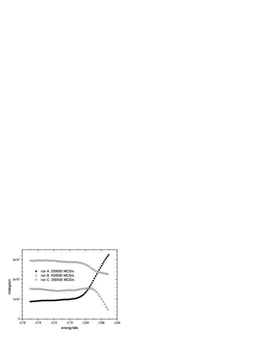
Figure 1: Convergence study in zone II. $L=24$, $h_{0}=2.1$, runs A and B are a second step iteration of the whole WL algorithm, run C is a third step. Doubling the maximum MCS/s number causes an important improvement in the flatness of the histogram (compare histogram A and B). However, it is more efficient to take the input of run A and re-run the WL algorithm (run C) (for the same total amount MCS/s). The region where the histogram is almost completely flat increases beyond that corresponding to run B. For clarity only some points of the histograms are plotted.

Run A has been performed with a maximum of 200000 MCS/s for each value of the WL factor and run B with 400000 MCS/s. The energy range where the energy histogram is flat is wider for the longer run, but it still doesn’t cover the whole sub-interval.

A better result is obtained with run C where the almost perfect flat region is extended beyond the one of run B. Run C has a maximum of 200000 MCS/s for each f-value but it is a third iteration step: the initial guess of the density of states is the $g(E)$ obtained from run A. So we see that for a given total amount of MCS/s, it is more efficient to perform two iteration steps of the whole WL algorithm with 200000 MCS/s each, than only one with 400000 MCS/s.

To further improve this convergence, we combine this third iteration step with an extra splitting of the energy subinterval in region II. In Figure 2 we compare the same run C already shown in figure 1 with three new runs performed in smaller overlapping energy intervals. The three of them are a third iteration steps with the same initial guess that run C. In this way we achieve convergence in region II.

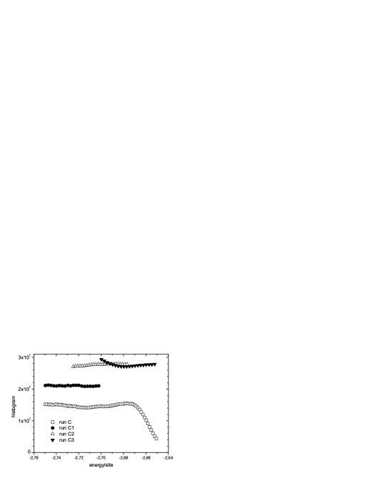
Figure 2: Convergence study in zone II. $L=24$, $h_{0}=2.1$, Here all the runs are a third iteration step (this means that the input was taken from run A). Comparison between the results issued from run C over the whole sub-interval and those obtained splitting the interval into three overlapping ones (C1,C2,C3). For clarity only some points of the histograms are plotted.

As usual, the global density of states $g(E),\forall E$ was built up by joining the different parts obtained in each interval.

3 Results

We have studied 3D lattices of linear size $L$=10, 16, 20, 24, 30. For a given size and $h_{0}$ value, different realizations (around 10) of the quenched disorder have been studied, each one of them is called a “sample” in the following. For some of these samples we have studied the behavior of the system as a function of $h_{0}$.

Our results show two clearly distinct critical behaviors according to the value of $h_{0}$.

For low $h_{0}$ values the specific heat curve as a function of temperature, $C(T)$, shows the characteristic peak of a second order transition in a finite system at a certain critical temperature $P_{T_{c}(L)}(E)$ (see figure 3). The corresponding probability density at $T_{c}(L)$ is shown in Figure 4. Only one peak is observed, indicating that the system is dominated by thermal fluctuations while the presence of the random field is only a small perturbation.

Figure 3: $L=24$, $h_{0}=0.5$ Specific heat as a function of temperature.

Figure 4: $L=24$, $h_{0}=0.5$ Single-peaked probability density at the critical temperature $T_{c}=4.34$

On the other hand, for higher fields the $C(T)$ curves may have more than one peak with, in general, a dominant peak, and a few secondary ones, as can be seen in figure 5.

Moreover, the position of these $C(T)$ peaks is sample-dependent, suggesting that each sample has its own transition temperature $T^{*}$. The consequence of these large sample to sample fluctuations is to prevent from performing a naive averaging over the quenched disorder.

Figure 5: $L=24$, $h_{0}=2.1$ Specific heat as a function of temperature. Multiple peaks appear, their locations and heights are sample-dependent.

The analysis of the $P_{T}(E)$ curves near the temperatures where the maxima of $C(T)$ are located provides an interpretation for this multiplicity of peaks.

In figure 6 we show the corresponding $P_{T}(E)$ curves for three different temperatures in the region of the highest peak of the specific heat of figure 5. A double peak structure clearly appears, showing the coexistence of states with different energies separated by an energy region where the probability is zero. The transition temperature $T^{*}$ may be determined by the temperature where the two peaks in $P_{T^{*}}(E)$ have equal height. Here it is $T^{*}\approx 2.19$. A qualitative study of the size effect shows that the double peak in $P_{T^{*}}(E)$ is present for $L\geq 16$, and enhances with size.

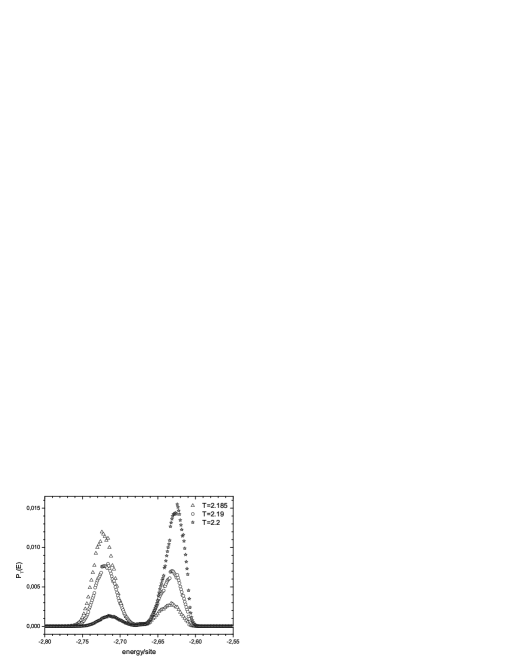
Figure 6: $L=24$, $h_{0}=2.1$ Double-peaked probability density at three temperatures in the transition region. It can be seen how the peak is shifted from low to high energy values as the temperature increases. The transition temperature may be estimated from these curves as the value where the two peaks have the same height (here $T=2.19$). For the sake of clarity only some points of the curves are plotted.

The shape of the $P_{T}(E)$ corresponding to the secondary peaks of the $C(T)$ is also far from the one characterizing a second order transition (see figures  4 and 7). It shows a structured peak, somehow similar to a double peak, but it should be noticed that the minimum in between the maxima does not go to zero. The same structure is found for the other secondary peaks.

This allows for an interpretation of the multiplicity of peaks in $C(T)$: they may indicate a region of meta-stable states where the system undergoes a reversal of large domains. This behaviour has also been found in [12].

The very existence of these metastable states, which are absent for a low value of $h_{0}$, supports the interpretation of the transition as first order. This situation is often found in standard Monte Carlo studies of systems undergoing first order transitions, where the dynamics is based on the canonical ensemble and the system risks to be trapped in a local minimum of the free energy. In these cases it is commonly observed that in a finite temperature region, there are jumps in the order parameter curves as a function of the temperature, with hysteresis in field cooling and field heating loops. Noteworthly, a trace of this situation if found here even though the dynamics of the W-L algorithm doesn’t suffer from metastabilities.

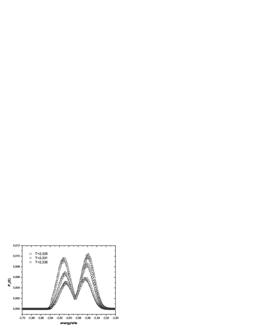
Figure 7: $L=24$, $h_{0}=2.1$ Probability density at three temperatures around a secondary peak of $C(T)$. There is a coexistence of energies with non zero probability, indicating the existence of meta-stable states separated by energy barriers of different heights. For the sake of clarity only some points of the curves are plotted.

Figure 8 shows the results of the study of a given sample for different intensities of the quenched disorder $h_{0}$. The behaviour clearly changes with the intensity of the random field: while $C(T)$ curves have only one peak for low field values, a second one appears, as the field increases. For high field the $C(T)$ curves show clearly more than one peak.

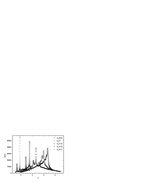
Figure 8: $L=24$, $h_{0}=0.5-2.1$. Specific heat as a function of the temperature for a single sample and different values of $h_{0}$. The curve clearly transforms from a single-peaked $C(T)$ curve characteristic of continuous transitions to a multi-peak curve where the position and multiplicity of the peaks are sample dependent

It must be stressed that, for high field values, the double peak in $P_{T^{*}}(E)$ is always present for all studied samples of sufficiently large sizes ( $L\geq 16$) . The position of the peaks may vary as they correspond to different $T^{*}$ (recall that $T^{*}$ is sample dependent).

4 Discussion

We have performed a WL study of the 3D-RFIM with a bimodal distribution of the random fields. Our results clearly show that the critical behavior of the system depends on the value of $h_{0}$. For low values of $h_{0}$ the transition has all the characteristics of a continuous one: we observed one peak in $C(T)$ curves at a critical temperature $T_{c}(L)$. The corresponding probability distribution of the energy at that temperature is single-peaked.

For high $h_{0}$ several indicators of a first order transition are observed. First $C(T)$ curves become irregular giving rise to secondary peaks when the field increases. These peaks have already been observed for the gaussian model and they have been related to the reversal of large spin domains. This is a phenomenon commonly encountered in standard Monte Carlo simulations of a magnetic systems undergoing first order transitions. The system goes through different meta-stable states when the conditions of the simulation are modified (typically in field heating and field cooling simulations). This gives rise to hysteresis loops. The passage from one meta-stable state to the other is done by the reversal of a large domain.

We have also found that the probability energy distribution at the transition temperature in this high field region is double-peaked, showing a coexistence of states of the same probability at a given temperature.

This work confirms the results reported in a previous article by one us [22]. It is interesting to remark that the same result is now obtained by a completely different calculation method. In fact, in [22] the bimodal RFIM has been studied using a combination of standard Monte Carlo (Metropolis) and histogram Monte Carlo simulations. Both simulations were performed in the canonical ensemble. As it is well known, simulations in the canonical ensemble may be affected by metastabilities near a first order phase transition as the system risks to be trapped in a local minimum of the free energy, due to the high energy barriers. In Ref.[22] for a given value of $h_{0}$, the energy probability distribution at the transition temperature was found to be double or single-peaked depending on the particular path the system followed in the phase space during its evolution.

In the present work, the states of the system are not sampled using the canonical ensemble. The WL algorithm gives an estimate of the density of states by performing a random walk on the energy space, so the system should not be trapped in a metastable state.

We also observe large sample to sample fluctuations in the location and the height of the specific heat maxima in agreement with Malakis et al. [24]. At a fixed size, each sample has its own critical temperature and even the number of secondary peaks of the specific heat depends on the sample. This implies that the average over disorder of any quantity $A(T)$ in order to locate the critical temperature for a given size, $T_{c}(L)$ is not meaningful. Moreover, by doing so all information concerning an eventual first order transition would be washed out. This has been the working method in previous works performing sample averaging, ie: [9] and it is perhaps one of the reasons for the remaining controversy.

Malakis et al. [24] pointed out the need to take into account the sample to sample fluctuations when performing averages over the quenched disorder. Nevertheless, in their work each sample has been studied using the technique of critical minimum energy subspace described in [26]. The method assumes a continuous transition. In fact it is based on the hypothesis of a gaussian-like energy distribution at the pseudo critical temperature and on the validity of second order finite size scaling relationships. These hypothesis are not valid when $P_{T}(E)$ is double peaked.

References

- [1] For a review see Yukito Iba, Intl. Journal of Mod. Phys. C 12, 623 (2001).
- [2] Fugao Wang and D.P.Landau, Phys. Rev. Lett. 86, 2050 (2001).
- [3] Fugao Wang and D.P.Landau, Phys. Rev. E 64, 056101-1 (2001).
- [4] Chenggang Zhou and R. N. Bhatt, Phys. Rev. E 72, 025701 (2001).
- [5] B. J. Schultz, K. Binder, M. Müller and D. P. Landau, Phys. Rev. E 67, 067102 (2003).
- [6] A. Malakis, S. S. Martinos, I. A. Hadjiagapiou and A. S. Peratzakis, Interational Journal of Modern Physics C 15, 729 (2004).
- [7] Chenggang Zhou, T. C. Schulthess, Stefan Torbrügge and D. P. Landau, Phys. Rev. Lett. 96, 120201 (2006)
- [8] Andrew T. Ogielski, Phys. Rev. Lett. 57, 1251(1986).
- [9] Heiko Rieger, Phys. Rev. B 52, 6659 (1995).
- [10] A.A. Middleton and D. Fisher, Phys. Rev. B 65, 134441 (2002).
- [11] I. Dukovski and J. Machta, Phys. Rev. B 67, 014413 (2003).
- [12] Y. Wu and J. Machta, Phys. Rev. Lett. 95, 137208 (2005)
- [13] Y. Wu and J. Machta, Phys. Rev. B 74, 064418 (2006)
- [14] Angles D’Auriac and Sourlas Europhys. Lett 39, 473 (1997).
- [15] Hartmann and U. Nowak, Europhys. Journal B 7, 105 (1999).
- [16] Hartmann and A. P. Young Phys. Rev. B 64, 214419 (2001).
- [17] S.R. McKay and A.N. Berker, J. Appl. Phys. 64, 5785 (1988).
- [18] Daniel S. Fisher, Phys. Rev. Lett. 56, 416 (1986).
- [19] Thierry Jolicoeur and Jean-Claude Le Guillou Phys. Rev.B 56, 10766 (1997).
- [20] Heiko Rieger, and A. P. Young J. of Phys. A 26, 5279 (1993).
- [21] A. Falicov, A.N. Berker, and S.R. McKay, Phys. Rev. B 51 , 8266 (1995)
- [22] Laura Hernandez and H. T. Diep, Phys. Rev.B 55, 14080 (1997).
- [23] Nikolaos G. Fytas and Anastasios Malakis, Eur. Phys. J. B 50, 39 (2006)
- [24] Anastasios Malakis and Nikolaos G. Fytas,Phys. Rev. E 73, 016109 (2006).
- [25] Simon Alder, Simon Trebst, Alexander K. Hartmann and Matthias Troyer, J. Stat. Mech. P07008 (2004).
- [26] A. Malakis, A. Peratzakis, and N. G. Fytas, Phys. Rev. E 70,066128 (2004).