Theoretical X-Ray Absorption Debye-Waller Factors

Abstract

An approach is presented for theoretical calculations of the Debye-Waller factors in x-ray absorption spectra. These factors are represented in terms of the cumulant expansion up to third order. They account respectively for the net thermal expansion $\sigma^{(1)}(T)$, the mean-square relative displacements $\sigma^{2}(T)$, and the asymmetry of the pair distribution function $\sigma^{(3)}(T)$. Similarly, we obtain Debye-Waller factors for x-ray and neutron scattering in terms of the mean-square vibrational amplitudes $u^{2}(T)$. Our method is based on density functional theory calculations of the dynamical matrix, together with an efficient Lanczos algorithm for projected phonon spectra within the quasi-harmonic approximation. Due to anharmonicity in the interatomic forces, the results are highly sensitive to variations in the equilibrium lattice constants, and hence to the choice of exchange-correlation potential. In order to treat this sensitivity, we introduce two prescriptions: one based on the local density approximation, and a second based on a modified generalized gradient approximation. Illustrative results for the leading cumulants are presented for several materials and compared with experiment and with correlated Einstein and Debye models. We also obtain Born-von Karman parameters and corrections due to perpendicular vibrations.

I Introduction

Thermal vibrations and disorder in x-ray absorption spectra (XAS) give rise to Debye-Waller (DW) factors varying as $\exp[-W(T)]$, where $W(T)\approx 2k^{2}\sigma^{2}(T)$ and $\sigma^{2}(T)$ is the mean square relative displacement (MSRD) of a given multiple-scattering (MS) path.Crozier et al. (1988) These Debye-Waller factors damp the spectra with respect to increasing temperature $T$ and wave number $k$ (or energy), and account for the observation that the x-ray absorption fine structure (XAFS), “melts” with increasing temperature.Shmidt (1963) The XAFS DW factor is analogous to that for x-ray and neutron diffraction or the Mößbauer effect, where $W(T)=(1/2)k^{2}u^{2}(T)$. The difference is that the XAFS DW factor refers to correlated averages over relative displacements, e.g., $\sigma^{2}=\langle[({\mathbf{u}}_{R}-{\mathbf{u}}_{0})\cdot{\hat{\mathbf{R}}}]^{2}\rangle$ for the MSRD, while that for x-ray and neutron diffraction refers to the mean-square displacements $u^{2}(T)=\langle({\bf u\cdot\hat{\bf R}}{})^{2}\rangle$ of a given atom. Due to their exponential damping, accurate DW factors are crucial to a quantitative treatment of x-ray absorption spectra. Consequently, the lack of precise Debye-Waller factors has been one of the biggest limitations to accurate structure determinations (e.g., coordination number and interatomic distances) from XAFS experiment.

Due to the difficulty of calculating the vibrational distribution function from first principles, XAFS Debye-Waller factors have, heretofore, been fitted to experimental data or estimated semi-empirically, e.g., from correlated Einstein and Debye models. Sevillano et al. (1979); Van Hung and Rehr (1997) However, these ad hoc approaches are unsatisfactory for several reasons. First, there are often many more DW factors in the MS path expansion than can be fit reliably. Second, semi-empirical models typically ignore anisotropic contributions and hence do not capture the detailed structure of the phonon spectra.

To address these problems, we introduce first principles procedures for calculations of the Debye-Waller factors in XAS and related spectra. Our approach is based primarily on density functional theory (DFT) calculations of the dynamical matrix, together with an efficient Lanczos algorithm for the projected phonon spectra.Poiarkova and Rehr (2001); Krappe and Rossner (2002) DFT calculations of crystallographic Debye-Waller factors and other thermodynamic quantities have been carried out previously using modern electronic structure codes, Baroni et al. (2001); Lee and Gonze (1995); Rignanese et al. (1996) and our work here builds on these developments, with particular emphasis on applications to XAS.

Due to intrinsic anharmonicity in the interatomic forces, the behavior of the DW factors is extremely sensitive to the equilibrium lattice constant $a$. For example, we find that $\sigma^{2}$ varies approximately as $a^{6\gamma}$, where $\gamma=-d\ln\bar{\omega}/d\ln V$ is the mean Grüneisen parameter which is typically about 2 for fcc metals, and $\bar{\omega}$ refers to the mean phonon frequency. Consequently $\sigma^{2}$ is also very sensitive to the choice of the exchange-correlation potential in the DFT, since a $1\%$ error in lattice constant yields an error of $6\gamma\approx 10\%$ in $\sigma^{2}$. As a result, relatively small errors in the lattice constant predicted by the local density approximation (LDA) which tends to overbind, or the generalized gradient approximation (GGA) which tends to underbind, become greatly magnified Narasimhan and de Gironcoli (2002) in DW calculations.

In order to treat this sensitivity we have developed two ad hoc prescriptions for ab initio calculations of Debye-Waller factors based on DFT calculations with I) the conventional LDA and II) a modified-GGA (termed hGGA) described below. For comparison we also present selected results with a conventional GGA, with the correlated Einstein and Debye models, and with an empirical model based on the Born-von Karman parameters obtained from fits to phonon spectra. Detailed results are presented for a number of fcc and diamond structures.

II Formalism

II.1 Cumulants

In this section we outline the formalism used in our approach. Physically, the DW factors in XAS arise from a thermal and configurational average of the XAS spectra $\langle\mu(E)\rangle$ over the pair (or MS path length) distribution function, where $\mu(E)$ is the x-ray absorption coefficient in the absence of disorder. The effects of disorder and vibrations are additive, but since the factors due to configurational disorder are dependent on sample history and preparation, in this paper we focus only on the thermal contribution. The effect of the DW factors on the XAFS $\chi(k)$ is dominated by the average over the oscillatory behavior of each path in the multiple-scattering (MS) path expansion $\chi_{R}(k)\propto\sin(2kR+\Phi)$. If the disorder is not too large the average is conveniently expressed in terms of the cumulant expansion,Kubo (1962); Crozier et al. (1988)

$$\left\langle e^{i2kr}\right\rangle \equiv e^{2ikR_{0}}e^{-W(T)},$$ (1)

$$W(T) = -\sum_{n=1}^{\infty}\frac{\left(2ik\right)^{n}}{n!}\sigma^{\left(n\right)}(T),$$ (2)

where $r$ is the instantaneous bond length, $R_{0}$ the equilibrium length in the absence of vibrations, and $\sigma^{\left(n\right)}(T)$ the $n$-th cumulant average. For multiple-scattering paths, this length refers to half the total MS path length. The dominant effect on XAFS amplitudes comes from the leading exponential decay factor $W(T)\approx 2k^{2}\sigma^{2}(T)$, while the imaginary terms in $W(T)$ contributes to the XAFS phase. The leading such contribution is the thermal expansion which comes from the first cumulant $\sigma^{(1)}(T)$

$$\sigma^{\left(1\right)}=\left\langle r-R_{0}\right\rangle.$$ (3)

Thus, the mean bond length is $\langle r\rangle\equiv\bar{r}=R_{0}+\sigma^{\left(1\right)}(T)$. The skew of the distribution, which is given by the third cumulant $\sigma^{(3)}(T)$ contributes a negative phase shift, and hence the mean distance obtained in fits to XAFS experiment is typically shorter than that obtained from the first cumulant alone.Crozier et al. (1988) As emphasized above, an accurate account of the effects of anharmonicity is key to a quantitative treatment of these DW factors over a broad range of temperatures. This is illustrated in Fig. 1, which shows the strong variation in the mean phonon frequency $\bar{\nu}=\bar{\omega}/2\pi$ vs small variations in lattice constant as calculated using various models described below.

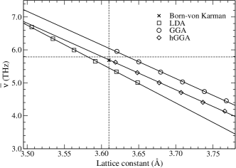
Figure 1: Mean frequency $\bar{\nu}$ of the VDOS projected along the nearest neighbor single scattering path of Cu, obtained from the first Lanczos iteration. The vertical line indicates the experimental lattice constant at 298 K while the horizontal line shows the Einstein frequency obtained from the experimentally determined DW factor. The Born-von Karman parameters for Cu at 298 K were taken from Ref. Nicklow et al., 1967.

The expressions for the higher cumulants in Eq. (1) simplify when expressed with respect to the mean, and are Crozier et al. (1988)

$$\sigma^{\left(2\right)} = \left\langle(r-\bar{r})^{2}\right\rangle\equiv\sigma^{2}\left(T\right),$$ (4a)

$$\sigma^{\left(3\right)} = \left\langle(r-\bar{r})^{3}\right\rangle.$$ (4b)

The thermal averages involved in the calculation of the cumulants can be expressed in terms of the projected vibrational density of states (VDOS) $\rho_{R}(\omega)$.Poiarkova and Rehr (1999, 2001); Krappe and Rossner (2002) For example, the MSRD $\sigma^{2}$ for a given path $R$ is given by the Debye integral

$$\sigma^{2}_{R}(T)=\frac{\hbar}{2\mu_{R}}\int_{0}^{\infty}{\frac{1}{\omega}\coth\Bigl{(}\frac{\beta\hbar\omega}{2}\Bigr{)}\rho_{R}\left(\omega\right)}~{}d\omega,$$ (5)

where $\mu_{R}$ is the reduced mass associated with the path, $\beta=1/k_{B}T$, and $\rho_{R}\left(\omega\right)$ is the vibrational density of states projected on $R$. In the following, the path index subscript $R$ is suppressed unless needed for clarity.

The first cumulant $\sigma^{(1)}$ is generally path-dependent and reflects the anharmonic behavior of a system. For monoatomic systems, this quantity is directly proportional to the net thermal expansion $\Delta a=a(T)-a_{0}$, which can be obtained by minimizing the vibrational free energy $F(a,T)$. Within the quasi-harmonic approximation, $F(a,T)$ is given by a sum over the internal energy $E(a)$ and the vibrational free energy per atom

$$\begin{split}F(a,T)=&E(a)+\\ &3k_{B}T\int_{0}^{\infty}d\omega\,\ln\left[{{2\sinh\left(\frac{\beta\hbar\omega}{2}\right)}}\right]\rho_{a}(\omega),\end{split}$$ (6)

where $T$ is the temperature, $\rho_{a}(\omega)$ is the total VDOS, and we have assumed cubic symmetry for simplicity.

Furthermore, as pointed out by Fornasini et al.,Fornasini et al. (2004) the values of the cumulants measured in XAFS experiments include two further corrections. First, perpendicular vibrations lead to a small increase in the mean expansion observed in XAFS compared to that in x-ray crystallography:

$$\Delta\sigma^{\left(1\right)}_{\perp}=\frac{1}{2R_{0}}\sigma^{2}_{\perp}.$$ (7)

We have shown (see Appendix) that $\sigma^{2}_{\perp}$ and $\sigma^{2}$ are closely related, and hence that $\sigma^{2}_{\perp}$ can be estimated in terms of $\sigma^{2}$. Second, the position dependent XAFS amplitude factors $\exp(-2R/\lambda)/R^{2}$ give rise to an effective radial distribution function $g(R)\rightarrow g(R)\exp(-2R/\lambda)/R^{2}$ which shifts thermal expansion observed in XAFS by an additional correction

$$\Delta\sigma^{\left(1\right)}=-\frac{2}{R}\left(1+\frac{R}{\lambda}\right)\sigma^{2}.$$ (8)

This second correction is often included in XAFS analysis routines and has been taken into account in the experimental results presented here.Fornasini et al. (2004) Note that the corrections in Eq. (7) and (8) are both of the same order of magnitude and partially cancel.

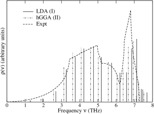
Figure 2: Total vibrational density of states of Cu at 49 K from DFT calculations using the LDA with our prescription I; the hGGA (see text) with our prescription II; and from experiment Nicklow et al. (1967).

II.2 Lanczos Algorithm

The VDOS $\rho_{R}\left(\omega\right)$ has often been approximated by means of Einstein and Debye models based on empirical data. Although these models are quite useful, especially for isotropic systems such as metals without highly directional bonds, their limitations are well known.Dimakis and Bunker (1998); Poiarkova and Rehr (1999) To overcome some of these limitations Poiarkova and Rehr Poiarkova and Rehr (1999, 2001) proposed a method in which the VDOS is calculated from the imaginary part of the lattice dynamical Green’s function

$$\rho_{R}(\omega)=-\frac{2\omega}{\pi}\mathrm{Im}\Bigl{<}0\Bigl{|}\frac{1}{\omega^{2}-{\bf D}+i\epsilon}\Bigr{|}0\Bigr{>}.$$ (9)

Here $\left|0\right>$ is a Lanczos seed vector representing a normalized, mass-weighted initial displacement of the atoms along the multiple-scattering path $R$, and ${\bf D}$ is the dynamical matrix of force constants

$$D_{jl\alpha,j^{\prime}l^{\prime}\beta}=\left(M_{j}M_{j^{\prime}}\right)^{-1/2}~{}\frac{\partial^{2}E(a)}{\partial u_{jl\alpha}\partial u_{j^{\prime}l^{\prime}\beta}}.$$ (10)

where $u_{jl\alpha}$ is the $\alpha=\left\{x,y,z\right\}$ Cartesian displacement of atom $j$ in unit cell $l$ and $M_{j}$ is the mass of atom $j$, and where $E(a)$ is the internal energy of the system evaluated at the lattice constant $a(T)$. Thus, our approach takes into account the main effects of anharmonicity in terms of force constants that depend parametrically on the temperature.

Efficient calculations of the lattice dynamical Green’s function can be accomplished using a continued fraction representation, with parameters obtained with the iterative Lanczos algorithm.Deuflhard and Hohmann (1995) This yields a many-pole representation for the VDOS which is well suited for accurate spectral integrations. The first step in the Lanczos algorithm corresponds to the correlated Einstein model,

$$\rho_{R}=\delta(\omega-\bar{\omega})$$ (11)

with an Einstein frequency $\bar{\omega}$ given by

$$\bar{\omega}^{2}=\langle 0|{\bf D}(R)|0\rangle.$$ (12)

The frequency $\bar{\omega}$ corresponds to the rms average over the projected phonon spectra $\rho(\omega)$. However, the choice of the Einstein frequency is not unique, and the appropriate choice depends on the physical quantity being calculated, as discussed in more detail below. Poiarkova et al. truncated the continued fraction at the second tier (i.e. second Lanczos iteration), which is usually adequate to converge the results to about 10%. Subsequently Krappe and Rossner Krappe and Rossner (2002) showed that at least six Lanczos iterations are required to achieve convergence to within $1\%$. Thus the Lanczos algorithm provides an efficient and accurate procedure for calculating MS path-dependent DW factors from Eq. (5).

The main difficulty in implementing the Lanczos algorithm lies in obtaining an accurate model for the dynamical matrix (or force constants) $\bf D$ for a given system. Although semi-empirical estimates of interatomic force constants or Born-von Karman parameters are sometimes available, their temperature dependence limits their accuracy and generality. Similarly, simple models for the vibrational distribution function (e.g., Einstein and Debye) generally ignore anisotropic behavior. One of our main aims in this paper is to develop a first principles approach that allows us to calculate the force constants for various systems using DFT. In addition, we have extended the Lanczos algorithm described above to several other cases by generalizing the Lanczos seed-state $\left|0\right>$. This allows us to calculate several other quantities including the total vibrational density of states (VDOS), the vibrational free energy, thermal expansion, the mean square atomic displacements $u^{2}(T)$ in crystallographic Debye-Waller factors.Rossner et al. (2006) In addition, we calculate $\sigma_{\perp}^{2}$, which yields the perpendicular motion contribution to the DW factor of Eq. (5), and estimates of the third cumulant. Representative results for the VDOS calculated by this method are illustrated in Fig. 2.

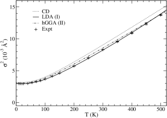
Figure 3: Temperature dependence of the Debye-Waller factor for the nearest neighbor single scattering path in Cu. The experimental difference values Fornasini et al. (2004) were shifted to match the LDA (I) results at 0 K.

II.3 Correlated Einstein Model

Although the cumulants other than the second are often negligible for small anharmonicity, their calculation using the apparatus of anharmonic lattice dynamics is computationally demanding. On the other hand, it has been shown that these cumulants can be approximated to reasonable accuracy using a correlated anharmonic Einstein model for each MS path,Frenkel and Rehr (1993); Van Hung and Rehr (1997) and this is the method adopted here. In this approach an Einstein model is constructed for each MS path keeping only cubic anharmonicity, yielding the effective one-dimensional potential

$$V(x)=\frac{1}{2}k_{0}x^{2}+k_{3}x^{3},$$ (13)

where $x$ is the net stretch in a given bond. The Einstein frequency $\omega_{E}$ within the quasi-harmonic approximation is then obtained from the relation Eq. (23), i.e., $k=k_{0}+6k_{3}\bar{x}=\mu\omega_{E}^{2}$. This choice of Einstein frequency ensures that the high temperature behavior of $\sigma^{2}$ from the Einstein model agrees with Eq. (5). The construction of this Einstein model from the dynamical matrix $\bf D$ along with explicit examples is given in the Appendix. The relations between the cumulants for the Einstein model can be used to obtain estimates for $\sigma^{(1)}$ and $\sigma^{(3)}$. For example, for the first cumulant

$$\sigma^{(1)}=-\eta\frac{3k_{3}}{k}\sigma^{2}.$$ (14)

Note that this relation differs from that in Refs. [Frenkel and Rehr, 1993; Van Hung and Rehr, 1997] in that it contains an extra multiplicative factor $\eta=1/\langle\omega^{-2}\rangle\bar{\omega}^{2}$, as discussed in the Appendix.

III DFT Calculations

III.1 Computational Strategy

As noted above, one of the main aims of this paper is to calculate the force constants within the quasi-harmonic approximation using DFT and an appropriate choice of exchange-correlation functional. Due to the extreme sensitivity of the phonon spectra to the interatomic distances, as discussed above, the most important parameters entering the calculation of the dynamical matrix are the lattice constant and the geometry of the system. A typical example of the effect of expansion is illustrated in Fig. 1, which shows the variation of the first moment of the VDOS (i.e. the average frequency $\bar{\nu}$) projected along the nearest-neighbor single-scattering path of Cu. For comparison Fig. 1 also shows $\bar{\nu}$ obtained with a model based on the Born-von Karman parameters at 298 K. As expected, when the system expands the vibrational frequencies are red-shifted due to the weakening of the interatomic interactions. From the common slopes in Fig. 1., we see that all of the functionals have similar Grüneisen parameters $\gamma\approx$ 2.2 at the experimental lattice constant 3.61 Å, in accord with the experimental valueCollins (1963) $2.0\pm 0.2$. Note that although at a given lattice constant the GGA functional always produces a stiffer model than LDA, i.e., with higher mean frequencies, the results at the equilibrium GGA lattice constant tend to be softer than at the equilibrium LDA lattice constant. Moreover, when compared with the experimental value, the LDA and GGA functionals respectively underestimate and overestimate the mean frequency by about 5%. This translates into a 20-25% error in the DW factors calculated with these methods. This margin of error is too large to make the DW factors of significant value in quantitative EXAFS analysis.

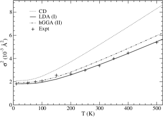
Figure 4: Temperature dependence of the Debye-Waller factor for the nearest neighbor single scattering path in Ge. The experimental difference values Dalba et al. (1999) were shifted to match the LDA (I) results at 0 K.

Based on the above considerations, we therefore propose two alternative prescriptions to stabilize our DW factor calculations:

I. Our first prescription is based on DFT calculations using the LDA exchange-correlation functional at the calculated equilibrium lattice constants $a(T)$ at a given temperature. Note however that the errors in the LDA estimates of the lattice constant are often larger than those obtained in fits to XAFS experiment.

II. Our second prescription is based on DFT calculations using a modified GGA exchange-correlation functional termed hGGA (with half-LDA and half-GGA) at the experimentally determined lattice constant $a(T)$ at a given temperature. As described below, this functional is constructed on the assumption that the “true” functional lies somewhere between pure LDA and GGA. This second prescription may be useful, for example, during fits of XAFS data to experiment, during which the interatomic distance is refined.

Clearly, the use of experimental structural parameters limits prescription II, since it requires the knowledge of the crystal structure at each of the temperatures of interest. Such information is only available a priori for a handful of systems, although it could be introduced as part of the fit procedure.

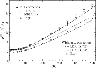
Figure 5: Temperature dependence of the first cumulant for the nearest neighbor single scattering path in Cu, with and without the perpendicular correction from Eq. 7, and obtained either from the minimization of the free energy (FE) or from the correlated Einstein model (EM). Both experimental difference values withFornasini et al. (2004) and withoutaip (1972) the perpendicular motion correction were shifted to match the LDA (I) results at 0 K.

III.2 Exchange-Correlation Functionals

In the course of this work, we investigated a number of exchange-correlation functionals. Generally, the exchange-correlation functional is attractive and hence strongly affects the overall strength and curvature of the interatomic potential. On the other hand it is well known that LDA functionals tend to overbind, yielding lattice constants smaller than experiment typically by about 1%. In contrast, GGA functionals tend to underbindNarasimhan and de Gironcoli (2002) by about the same amount. These errors are confirmed by our calculations, which show that for Cu the LDA yields a lattice constant of 3.57 Å at 0 K and 3.58 Å at 298 K, while the GGA yields 3.69 Å and 3.70 Å respectively, experiment being 3.61 Å. Moreover, the effect of the functionals on the phonon structure is even larger. For example, Narasimhan and de GironcoliNarasimhan and de Gironcoli (2002) show that the thermal expansion is about 10% high with LDA and 10% low with GGA.

Table 1: Born-von Karman parameters $D^{m}_{ij}$ (N/m) from neutron scattering compared with ab initio calculations from this work.

	m	ij	LDA	GGA	hGGA	Expt
	110	xx	$14.53$	$11.13$	$13.69$	$13.278$	[Nicklow et al., 1967]
Cu		zz	$-3.17$	$-2.18$	$-3.46$	$-1.351$
49 K		xy	$17.12$	$13.12$	$16.52$	$14.629$
	200	xx	$1.07$	$0.85$	$1.31$	$-0.041$
		yy	$-0.12$	$-0.11$	$-0.06$	$-0.198$
	110	xx	$10.46$	$6.03$	$12.98$	$10.71(17)$	[Kamitakahara and Brockhouse, 1969]
Ag		zz	$-3.28$	$-1.65$	$-4.11$	$1.75(20)$
296 K		xy	$12.48$	$7.27$	$15.94$	$12.32(32)$
	200	xx	$1.06$	$0.70$	$1.34$	$0.06(29)$
		yy	$-0.03$	$-0.08$	$-0.05$	$-0.23(19)$
	110	xx	$14.22$	$9.17$	$17.97$	$16.43(09)$	[Kamitakahara and Brockhouse, 1969]
Au		zz	$-7.51$	$-5.31$	$-8.78$	$-6.54(10)$
295 K		xy	$18.39$	$12.10$	$23.38$	$19.93(14)$
	200	xx	$3.96$	$3.30$	$4.42$	$4.04(17)$
		yy	$-0.33$	$-0.28$	$-0.25$	$-1.27(11)$
	110	xx	$29.17$	$23.67$	$29.94$	$25.681(168)$	[Dutton et al., 1972]
Pt		zz	$-7.60$	$-6.67$	$-8.77$	$-7.703(251)$
90 K		xy	$31.44$	$26.02$	$33.50$	$30.830(303)$
	200	xx	$4.98$	$4.67$	$5.18$	$5.604(329)$
		yy	$-1.56$	$-1.33$	$-1.28$	$-1.337(194)$

Although significant effort has been put into so-called meta-GGA functionalsTao et al. (2003); Staroverov et al. (2004) that address these issues, they have not yet been widely implemented. Therefore, to be consistent with various resultsNarasimhan and de Gironcoli (2002) and to preserve the advantages of the LDA and GGA functionals we have devised a modified functional termed hGGA which is a mixture of 50% LDA and 50% GGA, i.e., with a 50% reduction in both the additional exchange and correlation terms in the GGA. The motivation for the 50-50 mixture stems from the observation that the experimental values for many quantities are roughly bracketed by the LDA and GGA predictions. To simplify the development, we chose the closely related Perdew-Wang 92Perdew and Wang (1992) (LDA) and Perdew-Burke-ErnzerhofPerdew et al. (1996) (GGA) functionals. For this case the equal parts mixing can be achieved with two simple changes: First, the $\kappa$ parameter in the exchange energy term in PBE is reduced by half. This change preserves all the conditions on which PBE was founded, except the Lieb-Oxford bound. Second, the gradient contribution $H$ to the correlation energy is also reduced by half. Similar modified functionals for solids have been proposed by Perdew et al,Perdew (2007) suggesting that modifications similar to the hGGA may be more generally applicable. Fig. 1 shows the average frequency obtained with the hGGA functional and confirms that this yields the desired behavior.

Table 2: Debye-Waller factors $\sigma^{2}_{n}(T)$ (in $10^{-3}$ Ų) for the single scattering path to the n^th shell of some fcc lattice metals. The experimental difference values were shifted to match the LDA (I) at 80 K and the experimental error (in parentheses) indicates the error in the least significant digits.

	n	CD	LDA(I)	GGA	hGGA(II)	Expt
Cu	1	$6.11$	$5.48$	$6.79$	$5.80$	$5.57(05)$	[Stern et al., 1980]
190 K	2	$7.49$	$7.49$	$9.20$	$8.01$	$7.4(3)$
	3	$7.67$	$7.06$	$8.70$	$7.53$	$6.7(3)$
	4	$7.76$	$7.02$	$8.68$	$7.48$	$7.0(5)$
Cu	1	$9.04$	$8.22$	$10.45$	$8.56$	$7.99(16)$	[Stern et al., 1980]
300 K	2	$11.16$	$11.44$	$14.31$	$12.03$	$11.2(5)$
	3	$11.50$	$10.76$	$13.53$	$11.28$	$9.7(6)$
	4	$11.66$	$10.70$	$13.49$	$11.20$	$11.4(10)$
Pt	1	$3.55$	$3.23$	$3.91$	$3.23$	$3.22(05)$	[Stern et al., 1980]
190 K	2	$4.38$	$4.64$	$5.57$	$4.78$	$4.7(3)$
	3	$4.50$	$4.44$	$5.36$	$4.49$	$4.3(4)$
	4	$4.56$	$4.60$	$5.55$	$4.66$	$4.5(4)$
Pt	1	$5.41$	$4.98$	$6.08$	$4.90$	$4.83(05)$	[Stern et al., 1980]
300 K	2	$6.69$	$7.23$	$8.71$	$7.34$	$6.8(5)$
	3	$6.91$	$6.92$	$8.40$	$6.89$	$6.7(6)$
	4	$7.01$	$7.17$	$8.71$	$7.16$	$7.0(6)$
Ag	1	$3.78$	$3.69$	$4.89$	$3.38$	$3.9(3)$	[Newville, 1995]
80 K	2	$4.56$	$4.97$	$6.57$	$4.60$	$5.4(5)$
	3	$4.62$	$4.70$	$5.92$	$4.32$	$4.9(5)$
	4	$4.64$	$4.67$	$6.22$	$4.28$	$5.5(5)$

III.3 Dynamical Matrix

The key physical quantity needed in calculations of the Debye-Waller factors is the dynamical matrix $\bf D$. With modern electronic structure codes this matrix of force constants can be calculated with sufficient accuracy from first principles both for periodic and molecular systems.Baroni et al. (2001); Lee and Gonze (1995); Rignanese et al. (1996) In this paper we restrict our attention to periodic systems which can be treated, for example, using the methodology implemented in the ABINIT Gonze et al. (2002) code, as described in detail in Ref.  Gonze and Lee, 1997. Briefly, the reciprocal space dynamical matrix

$$\tilde{D}_{j\alpha j^{\prime}\beta}\left(\mathbf{q}\right)=\sum_{l^{\prime}}D_{j0\alpha,j^{\prime}l^{\prime}\beta}e^{i\mathbf{q}\cdot\left(\mathbf{R}_{j^{\prime}l^{\prime}}-\mathbf{R}_{j0}\right)}$$ (15)

is calculated in a $4\times 4\times 4$ grid of ${\bf q}$-vectors. This grid is interpolated inside the Brillouin zone and the real-space force constants are obtained by means of an inverse Fourier transform. We find that such an interpolated grid gives well converged real-space force constants up to the fourth or fifth shell. The neglect of the shells beyond that introduces an error much smaller than other sources of error in the method. Finally, since the calculation of the DW factors uses clusters that typically include about 20 shells, the full force constant matrix for these clusters must be built by replicating the $3\times 3$ $D_{jl\alpha,j^{\prime}l^{\prime}\beta}$ blocks obtained for each $jl,j^{\prime}l^{\prime}$ pair.

Table 3: Debye-Waller factors $\sigma^{2}_{n}(T)$ (in $10^{-3}$ Ų) for the single scattering path for the n^th shell of some diamond lattice semiconductors. The experimental difference values were shifted to match the LDA (I) at 80 K and the experimental error (in parentheses) indicates the error in the least significant digits.

	n	CD	LDA(I)	GGA	hGGA(II)	Expt
Ge	1	$5.11$	$3.42$	$3.98$	$3.76$	$3.5(1)$	[Stern et al., 1980]
295 K	2	$7.43$	$10.38$	$11.91$	$9.70$	$9.6(8)$
	3	$7.64$	$13.09$	$15.03$	$11.84$
GaAs	1	$5.17$	$3.97$	$4.59$	$3.86$	$4.2(1)$	[Stern et al., 1980]
295 K	2	$7.75$	$12.70$	$14.28$	$12.01$	$11.7(14)$
(Ga Edge)	3	$7.69$	$14.91$	$16.29$	$14.01$
GaAs	1	$5.15$	$3.96$	$4.59$	$3.86$	$4.2(1)$	[Stern et al., 1980]
295 K	2	$7.20$	$10.80$	$11.69$	$10.19$	$9.6(11)$
(As Edge)	3	$7.68$	$14.83$	$16.66$	$14.00$

III.4 Lattice and Force Constants

The temperature-dependent lattice constant $a(T)$ is obtained by minimizing $F(a,T)$ in Eq. (6) with respect to $a$ at a given temperature $T$. Within the electronic structure code ABINIT, the total VDOS $\rho_{a}(\omega)$ is calculated with histogram sampling in $\mathbf{q}$-space. However, we find it more convenient here to use a Lanczos algorithm in real space, similar to the approach used for the MSRD. This can be done by modifying the initial normalized displacement state $\left|0\right>$ in Eq. (9) to that for a single atomic displacement, rather than the displacement along a given MS path. If more than one atom is present in the unit cell the contributions from each atom must be calculated and added. Similarly for anisotropic systems one must trace over three orthogonal initial displacements. Fig. 2 shows a typical VDOS generated using the Lanczos algorithm. We find the free energies calculated with this approach deviate from the $\mathbf{q}$-space histogram method by less then 2 meV, i.e., to within 1%.

To minimize $F(a,T)$ efficiently we proceed as follows: First, the lattice constant is optimized with respect to the internal energy $E(a)$ and a potential energy surface (PES) for the cell expansion is built around the minimum. Second, the ab initio force constants are computed at each point of the PES to obtain the vibrational component of $F(a,T)$. Since this is the most time-consuming part of the calculation, we have taken advantage of the approximately linear behavior for small variations as illustrated in Fig. 1. Then, each element of the force constants matrix is interpolated according to

$$D_{jl\alpha,j^{\prime}l^{\prime}\beta}=A_{jl\alpha,j^{\prime}l^{\prime}\beta}+B_{jl\alpha,j^{\prime}l^{\prime}\beta}~{}\Delta a$$ (16)

from just two ab initio force constant calculations with slightly different lattice parameters. This interpolation scheme allows us to reduce the computational cost of a typical calculation by a factor of 2/3, while introducing an error of less than 2% in the average frequencies. Once the values of $F(a,T)$ on the PES are obtained, we determine the minimum $a(T)$ by fitting $F(a,T)$ to a Morse potential

$$F(a,T)=D_{0}\left[e^{-2\beta(a-a(T))}-2e^{-\beta(a-a(T))}\right].$$ (17)

We have estimated that the numerical error in this minimization is of order $5\times 10^{-4}$ Å or less by fitting only the internal energy component $E(a)$ and comparing with the minima obtained using conjugate gradient optimization.

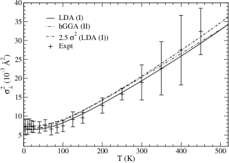
Figure 6: Temperature dependence of the perpendicular component $\sigma_{\perp}^{2}$ of the Debye-Waller factor for the nearest neighbor single scattering path in Cu. For comparison we also plot $2.5~{}\sigma^{2}$ to show the correlation $\sigma_{\perp}^{2}\approx\gamma_{\perp}\sigma^{2}$, together with the values extracted from experiment.Fornasini et al. (2004)

III.5 Computational Details

All the ABINIT calculations reported here use Troullier-Martins scheme—Fritz-Haber-Institut pseudopotentials. We found that an $8\times 8\times 8$ Monkhorst-Pack $k$-point grid and an energy cutoff of 60 au (12 au for Ge) were sufficient to achieve convergence with respect to the DW factors. In all cases where the geometries were varied, an energy cutoff smearing of 5% was included to avoid problems induced by the change in the number of plane wave basis sets. For metallic systems, the occupation numbers were smeared with the Methfessel and Paxton Methfessel and Paxton (1989) scheme with broadening parameter 0.025. Results are presented for LDA (Perdew-Wang 92Perdew and Wang (1992)) and GGA (Perdew-Burke-ErnzerhofPerdew et al. (1996)) functionals, as well as for our mixed hGGA functional.

IV Results

IV.1 Born-von Karman parameters

Phonon dispersion curves are often parametrized in terms of so-called Born-von Karman (BvK) coupling constants. These parameters are essentially the Cartesian elements of the real space dynamical matrix defined in Eq. (10). The main difference between the Born-von Karman parameters and force constants obtained within the quasi-harmonic approximation is that the former are tabulated at specific temperatures while the temperature dependence of the quasi-harmonic model arises implicitly from the dependence of the lattice parameters on thermal expansion. The dominant BvK coupling constants (up to the second neighbor) are presented in Table 1.

We find that both the LDA with prescription I and the hGGA with prescription II generally give force constants that are within a few percent of experiment. Typically the LDA force constants with prescription I are slightly higher than those from the hGGA with prescription II. Also, note that the transverse components of the BvK parameters tend to be overestimated. We have also considered the pure PBE GGA functionals, but find that they produce force constants that are significantly weaker due to their larger equilibrium lattice constants (Fig. 1).

IV.2 Mean-square Relative Displacements

Calculations of the MSRD for the dominant first near neighbor path for fcc Cu are shown in Fig. 3, and detailed results for various scattering paths are presented in Table 2. Both of our prescriptions I and II yield results in good agreement with experiment. For Cu even the correlated Debye model is quite accurate. Note also a slight deviation from linearity in temperature $T$ due to the variation in the dynamical matrix with temperature is visible both in the experimental curve and in the calculation using prescription I.

Similarly, calculations of the MSRD for the first neighbor path in Ge are shown in Fig. 4, and detailed results for various scattering paths are given in Table 3. Again, both of our prescriptions yield results in good agreement with experiment, with the LDA prescription being slightly better. For this case, however, the correlated Debye model is significantly in error; this is not unexpected given the strong anisotropy of the diamond lattice. Tables 2 and 3 also include similar results for Ag, Pt and GaAs.

IV.3 Thermal Expansion

The thermal expansion can now be calculated in two ways. First, by minimizing the free energy of the system using Eq. (6) one can obtain the overall thermal expansion corresponding to the expansion of the lattice constant $a(T)$. For monoatomic systems the thermal expansion of any MS path is simply proportional to the lattice constant. More generally, the expansion is MS path dependent, and can be estimated using the correlated Einstein model of II.3 and the Appendix. From Eq. (14) and the Einstein model Grüneisen parameter $\gamma=-k_{3}R/k$, this model predicts that the first cumulant $\sigma^{(1)}$ has a temperature dependence proportional to $\sigma^{2}/R$,

$$\sigma^{(1)}={\frac{3\gamma\eta}{R}}\sigma^{2},$$ (18)

As shown in Fig. 5 (dashed and dotted curves), this correlated Einstein model estimate for the thermal expansion agrees well with that obtained from minimizing the free energy of the system and with experimental crystallographic data.

IV.4 Perpendicular Motion Contributions

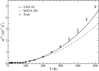
Figure 7: Temperature dependence of the third cumulant for the nearest neighbor single scattering path in Cu. The experimental difference valuesFornasini et al. (2004) were shifted to match the LDA (I) results at 0 K.

Fig. 5 also shows the first cumulant for Cu obtained by adding the crystallographic component $\sigma^{(1)}=\bar{x}$ and the correction due to perpendicular motion $\Delta\sigma^{(1)}_{\perp}$ from Eq. (7). As observed by Fornasini et al.,Fornasini et al. (2004) the mean square perpendicular motion (MSPD) is correlated with $\sigma^{2}$, i.e., $\sigma_{\perp}^{2}=\gamma_{\perp}\sigma^{2}$, with an observed proportionality constant for Cu $\gamma_{\perp}\approx 2.5\pm 0.3$.Fornasini (in press, 2007) The MSPD can be calculated using our Lanczos procedure with an appropriately modified seed state $|0\rangle$ for perpendicular vibrations. This yields a ratio for $\gamma_{\perp}$ that varies from 2.17 to 2.36 between 0 and 500 K, respectively, for Cu. Moreover, as shown in the Appendix, this ratio can also be estimated using a correlated Einstein model for fcc structures, and we derive a value of 2.5 at high temperatures. The correlated Einstein model also predicts that $\gamma_{\perp}$ is weakly temperature-dependent, reducing to about $\sqrt{5}\approx 2.24$ at low temperature. We also show that for fcc structures the correction due to perpendicular motion is smaller than the crystallographic contribution by a factor of $\gamma_{\perp}/6\gamma$, which for Cu is about 20%. To illustrate this correlation, Fig. 6 shows the perpendicular motion contribution $\sigma_{\perp}^{2}$ calculated both by the Lanczos procedure and with a constant correlation factor $\gamma_{\perp}=2.5$.

We have carried out similar calculations of $\sigma_{\perp}^{2}$ for the case of diamond lattices. Due to the strongly directional bonding in diamond structures, and non-negligible bond bending forces, the calculations are more complicated than for fcc materials. Our ab initio calculations using the LDA with prescription I yield a ratio that varies from 3.4 to 7.2 between 0 and 600 K, in reasonable agreement with experiment where $\gamma_{\perp}$ varies between 3.5$\pm$0.6 and 6.5$\pm$0.5 in the same range. Fornasini (in press, 2007) In contrast our single near neighbor spring model (Appendix) gives a smaller high temperature value $\gamma_{\perp}=3.5$ and the addition of a single bond-bending parameter does not improve the agreement.

IV.5 Third Cumulant

As for the first cumulant, the third cumulant can be estimated from the correlated Einstein model, and the relation

$$\sigma^{(3)}=\eta\left[2-\frac{4}{3}\left(\frac{\sigma^{2}_{0}}{\sigma^{2}}\right)^{2}\right]\sigma^{(1)}\sigma^{2}.$$ (19)

Again an additional scaling factor $\eta$ is needed to correct the original Einstein model relations when $\sigma^{(1)}$ and $\sigma^{2}$ are replaced by the full results from our LDA calculations. Also the presence of this factor $\eta$ gives another correction to the relation $\sigma^{(1)}\sigma^{2}/\sigma^{(3)}\approx 2$ given by classical modelsStern et al. (1991) or the correlated Einstein model at high temperatures.

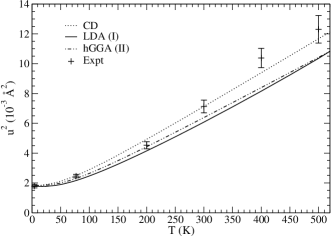
Figure 8: Temperature dependence of the crystallographic Debye-Waller factor for the nearest neighbor single scattering path in Cu, and compared to experimental values Flinn et al. (1961).

IV.6 Crystallographic Debye-Waller Factors

Finally, we present results for the x-ray and neutron crystallographic Debye Waller factors $W(T)=(1/2)k^{2}u^{2}(T)$, where the mean-square displacements $u^{2}(T)=\langle({\bf u\cdot\hat{\bf R}}{})^{2}\rangle$ are given by Eq. (5), with $\rho_{a}(\omega)$ given by the total vibrational density of states per site, as calculated by our Lanczos algorithm with an appropriate seed state.Rossner et al. (2006) For this case good agreement is obtained for both of our DFT prescriptions at low temperature, although the errors become more significant at higher temperatures. Also, we find that the convergence of the Lanczos algorithm is slower than for the path dependent Debye-Waller factors, requiring approximately 16 iterations to achieve convergence to 1%.

V Discussion and Conclusions

We have developed a first principles approach for calculations of the Debye-Waller factors in various x-ray spectroscopies, based on DFT calculations of the dynamical matrix and phonon spectra for a given system. We find that the results depend strongly on the choice of exchange-correlation potential in the DFT, but we have developed two prescriptions that yield stable results, one based on the LDA and one based on a modified GGA termed hGGA. Calculations for the crystalline systems presented here show that our LDA prescription yields good agreement with experiment for all quantities, typically within about $\pm$ 10%. Second, if the lattice constant is known a priori, our hGGA prescription also provides an accurate procedure to estimate the MSRD. Anharmonic corrections and estimates of the contribution from perpendicular vibrations are estimated using a correlated Einstein model. For these anharmonic quantities, however, we have found that the comparative softness of the lattice dynamics with the GGA and hGGA functionals leads to results which are somewhat less accurate than those for the LDA. Finally we have also calculated the crystallographic Debye Waller factors. Our approach also yields good results for calculations of DW factors in anisotropic systems, as illustrated for for Ge and GaAs. All of these results demonstrate that the prescriptions developed herein can yield quantitative estimates of Debye-Waller factors including anharmonic effects in various crystalline systems, and generally improve on phenomenological models. Extensions to molecular systems are in progress.

*

Appendix A

In this Appendix we briefly discuss the correlated Einstein model used in estimating anharmonic contributions to the DW factors. The model is illustrated with an application to the correlated Einstein model for calculating the mean-square radial displacement (MSRD) $\sigma^{2}$ and mean square perpendicular displacement (MSPD) $\sigma_{\perp}^{2}=\langle|\Delta\vec{u}_{\perp}|^{2}\rangle$.

The construction of Einstein models is not unique in that different physical quantities reflect different averages over the VDOS. For example, the theoretical MSRD given by Eq. (5) reflects an average over a thermal weight factor varying as $1/\omega^{2}$ at high temperatures. Thus the Einstein model parameters in our prescription are constructed to preserve the correct high temperature behavior of $\sigma^{2}$.Sevillano et al. (1979); Crozier et al. (1988) The first step in this construction is the calculation of $\bar{\omega}^{2}$ from the total potential energy for a net displacement $x$ of a path along a particular seed displacement state $|0\rangle$. Next this value is renormalized to give the correct MSRD at high temperatures. Thus we define

$$k_{0}=\eta\mu\langle 0|{\bf D}|0\rangle$$ (20)

where $\bar{\omega}^{2}$ is given from Eq. (12) and the factor $\eta=1/\langle\omega^{-2}\rangle\bar{\omega}^{2}$, where $\langle\omega^{-2}\rangle$ is the inverse second moment of the projected VDOS. The cubic coupling $k_{3}$ is then defined to be consistent with the variation in $k$ given by the Grüneisen parameter

$$\gamma=\frac{d\ln\bar{\omega}}{d\ln{R^{3}}}=-\frac{k_{3}R}{k}.$$ (21)

and hence must be is similarly renormalized

$$k_{3}=\frac{\eta}{6}\frac{d}{dR}\langle 0|{\bf D}(R)|0\rangle.$$ (22)

Then the Einstein frequency $\omega_{E}$ in the quasi-harmonic approximation is obtained from the relationFrenkel and Rehr (1993)

$$k=k_{0}+6k_{3}\bar{x}=\mu\omega_{E}^{2}.$$ (23)

where $\mu$ is the reduced mass. For Cu using the LDA (I) prescription for the dynamical matrix, this procedure yields $\eta=0.73$, $k_{0}=54.7$ N/m, $k_{3}=-48.4$ N/mÅ, and $k=51.1$ N/m.

The scaling factor $\eta$ thus forces the relation $\sigma^{2}(T)\rightarrow\sigma_{E}^{2}(T)=k_{B}T/\mu\omega_{E}^{2}$ at high temperature, where $\sigma^{2}(T)$ in the Einstein model is

$$\sigma_{E}^{2}(T)=\sigma^{2}_{0}\coth\left(\frac{\beta\hbar\omega_{E}}{2}\right),$$ (24)

and the zero-point value $\sigma_{0}^{2}=\sigma^{2}(0)=\hbar\omega_{E}/2k$.

Then, from $\sigma^{2}$ and relations between the cumulants,Frenkel and Rehr (1993); Van Hung and Rehr (1997) one can obtain MS path-dependent estimates for $\sigma^{(1)}$ and $\sigma^{(3)}$. When these relations are expressed in terms of the calculated (or experimental) values of the cumulants, we have found it necessary to include multiplicative factors of $\eta$ compared to the pure Einstein model expressions,Frenkel and Rehr (1993); Van Hung and Rehr (1997) to obtain quantitative agreement with experimental results e.g., as shown in Figs. 5 and 7.

As a second example, we construct such a model for monoatomic fcc Cu starting from an anharmonic pair potential. That is, we will assume that the lattice dynamics can be described by an anharmonic pair potential $V_{0}$ between near-neighbor bonds of the form

$$V_{0}(x)\cong\frac{1}{2}k^{0}x^{2}+k^{0}_{3}x^{3}.$$ (25)

Here $x$ is the net displacement $x$ along the bond direction, with positive displacements referring to expansion and negative to compression. Frenkel and Rehr (1993); Van Hung and Rehr (1997)

First consider the potential energy $V_{\parallel}(x)$ for vibrational displacement $x$ along the bond $(0R)$ between lattice points $(0,0,0)$ and $\vec{R}=R(0,1,1)/\sqrt{2}$. The net anharmonic potential $V_{\parallel}(x)$ is then given by Eq. (13) with a displacement state $x|0\rangle$ defined by $\vec{u}_{0}=(x/2)(0,1,1)/\sqrt{2}$, and $\vec{u}_{R}=(-x/2)(0,1,1)/\sqrt{2}$. Then constructing the dynamical matrix using Eq. (25) with small displacements, we find a net spring constant $k_{0}=\eta\langle 0|D|0\rangle=(5\eta/2)k^{0}$, in agreement with Ref. Van Hung and Rehr, 1997. This result can alternatively be obtained by summing the 23 pair potentials between the shared bond $(0R)$, the 11 nearest neighbor bonds to the origin and the 11 other nearest neighbor bonds to $R$, giving $V_{\parallel}(x)=V_{0}(x)+2V_{0}(-x/2)+8V_{0}(x/4)+8V_{0}(-x/4)+4V_{0}(0)$. Similarly we find that the anharmonic coupling [cf. Eq. (22)] is $k_{3}=(3\eta/4)k_{3}^{0}$, so that

$$V_{\parallel}(x)=\frac{1}{2}\left(\frac{5\eta}{2}k^{0}\right)x^{2}+\left(\frac{3\eta}{4}k^{0}_{3}\right)x^{3},$$ (26)

where we have again included a factor $\eta$ so that the Einstein model for $\sigma^{2}$ agrees with the expression from the inverse second moment of the VDOS.

In a similar way, we can develop a correlated Einstein model to describe the perpendicular vibrations. For this case we consider a vibrational displacement $\Delta\vec{u}_{\perp}$ of length $y=|\Delta\vec{u}_{\perp}|$ perpendicular to the bond between $(0,R)$. Thus we set $\vec{u}_{0}=(y/2)(0,1,-1)/\sqrt{2}$ and $\vec{u}_{R}=(-y/2)(0,1,-1)/\sqrt{2}$, where $R$ is the nearest neighbor distance. The net potential $V_{\perp}(y)$ is again obtained by summing the 23 pair potentials between the shared bond $(0R)$, the 11 nearest neighbor bonds to the origin and 11 others to $R$, similar to the calculation above for vibrations along the bond. For this case, two bonds are stretched by $y/2$, two contracted by $y/2$, three unchanged, eight stretched by $y/4$, and eight contracted by $y/4$, yielding a net sum $V_{\perp}(y)=2V_{0}(y/2)+2V_{0}(-y/2)+8V_{0}(y/4)+8V_{0}(-y/4)+3V_{0}(0)$, and hence

$$V_{\perp}(y)=\frac{1}{2}(2\eta k^{0})y^{2}.$$ (27)

Note that by symmetry, the net cubic anharmonic contribution vanishes. Thus the effective spring constant for the MSPD is $k=2\eta k^{0}$ and predicted to be insensitive to thermal expansion. The correlated Einstein model $V_{\perp}(z)$ is clearly the same for the MSPD along the $z$-axis,

With these results we can show that the MSPD for the first neighbor path in fcc materials $\sigma_{\perp}^{2}$ is correlated with $\sigma^{2}=\langle|\Delta\vec{u}_{\parallel}|^{2}\rangle$. Both the MSPD and MSRD in the Einstein model are given by Eq. 24, with their respective Einstein frequencies $\omega_{E}=(k/\mu)^{1/2}$. For the total contribution from perpendicular vibrations, one has to multiply by two to get the net $\sigma_{\perp}^{2}$ from both independent axes. At high temperatures for example, we obtain the MSPD $\sigma_{\perp}^{2}=2k_{B}T/2\eta k^{0}$. This is higher than the MSRD $\sigma^{2}=(2/5)k_{B}T/\eta k^{0}$ by a factor of $\gamma_{\perp}=5/2.$ The model also predicts a weakly temperature dependent ratio

$$\gamma_{\perp}(T)={\frac{\sigma_{\perp}^{2}(T)}{\sigma^{2}(T)}}=2\frac{\omega_{E}\coth(\beta\hbar\omega_{E}^{\perp}/2)}{\omega_{E}^{\perp}\coth(\beta\hbar\omega_{E}/2)}.$$ (28)

This ratio varies between $\sqrt{5}=2.236$ and 2.5 with increasing temperature. Thus the ratio $\gamma_{\perp}$ obtained with the correlated Einstein model, for the fcc lattice depends only on geometry and describes the anisotropy of the vibrational ellipsoid in monoatomic fcc structures reasonably well.

Because of the above relation between $\sigma_{\perp}^{2}$ and $\sigma^{2}$ in the Einstein model, the perpendicular motion correction can be related to the contribution to lattice expansion from anharmonicity. Thus from Eq. (7) and Eq. (18), we find that

$${\Delta\sigma^{(1)}_{\perp}}/{\sigma^{(1)}}={\gamma_{\perp}}/{6\eta\gamma}.$$ (29)

For fcc Cu this ratio predicts a correction to the first cumulant $\sigma^{(1)}$ from perpendicular motion of about 25%. Indeed, this shift is comparable to the observed differences in the thermal expansion with and without the perpendicular motion correction observed in Fig. 5. Thus for the dominant near neighbor bonds, the correlated Einstein model predicts a comparatively small but non-negligible effect of perpendicular motion on EXAFS distance determinations.

References

- Crozier et al. (1988) E. D. Crozier, J. J. Rehr, and R. Ingalls, in X-Ray Absorption: Principles, Applications, Techniques of EXAFS, SEXAFS, and XANES, edited by D. C. Koningsberger and R. Prins (Wiley, New York, 1988), p. 375.
- Shmidt (1963) V. V. Shmidt, Bull. Acad. Sci. USSR, Phys. Ser. 27, 392 (1963).
- Sevillano et al. (1979) E. Sevillano, H. Meuth, and J. J. Rehr, Phys. Rev. B 20, 4908 (1979).
- Van Hung and Rehr (1997) N. Van Hung and J. J. Rehr, Phys. Rev. B 56, 43 (1997).
- Poiarkova and Rehr (2001) A. Poiarkova and J. J. Rehr, J. Synchrotron Radiat. 8, 313 (2001).
- Krappe and Rossner (2002) H. J. Krappe and H. H. Rossner, Phys. Rev. B 66, 184303 (2002).
- Baroni et al. (2001) S. Baroni, S. de Gironcoli, A. Dal Corso, and P. Giannozzi, Rev. Mod. Phys. 73, 515 (2001).
- Lee and Gonze (1995) C. Lee and X. Gonze, Phys. Rev. B 51, 8610 (1995).
- Rignanese et al. (1996) G.-M. Rignanese, J.-P. Michenaud, and X. Gonze, Phys. Rev. B 53, 4488 (1996).
- Narasimhan and de Gironcoli (2002) S. Narasimhan and S. de Gironcoli, Phys. Rev. B 65, 064302 (2002).
- Kubo (1962) R. Kubo, J. Phys. Soc. Jpn 17, 1100 (1962).
- Nicklow et al. (1967) R. M. Nicklow, G. Gilat, H. G. Smith, L. J. Raubenheimer, and M. K. Wilkinson, Phys. Rev. 164, 922 (1967).
- Poiarkova and Rehr (1999) A. V. Poiarkova and J. J. Rehr, Phys. Rev. B 59, 948 (1999).
- Fornasini et al. (2004) P. Fornasini, S. a Beccara, G. Dalba, R. Grisenti, A. Sanson, M. Vaccari, and F. Rocca, Physical Review B (Condensed Matter and Materials Physics) 70, 174301 (pages 12) (2004), URL http://link.aps.org/abstract/PRB/v70/e174301.
- Dimakis and Bunker (1998) N. Dimakis and G. Bunker, Phys. Rev. B 58, 2467 (1998).
- Deuflhard and Hohmann (1995) P. Deuflhard and A. Hohmann, Numerical Analysis (de Gruyter, Berlin, 1995).
- Rossner et al. (2006) H. H. Rossner, , D. Schmitz, P. Imperia, H. J. Krappe, and J. J. Rehr, Phys. Rev. B 74, 134107 (2006).
- Frenkel and Rehr (1993) A. I. Frenkel and J. J. Rehr, Phys. Rev. B 48, 585 (1993).
- Collins (1963) J. G. Collins, Phil. Mag. 8, 323 (1963).
- Dalba et al. (1999) G. Dalba, P. Fornasini, R. Grisenti, and J. Purans, Phys. Rev. Lett. 82, 4240 (1999).
- aip (1972) American Institute of Physics Handbook (McGraw-Hill, New York, 1972).
- Kamitakahara and Brockhouse (1969) W. A. Kamitakahara and B. N. Brockhouse, Phys. Lett. A 29, 639 (1969).
- Dutton et al. (1972) D. H. Dutton, B. N. Brockhouse, and A. P. Miiller, Can. J. of Phys. 50, 2915 (1972).
- Tao et al. (2003) J. Tao, J. P. Perdew, V. N. Staroverov, and G. E. Scuseria, Phys. Rev. Lett. 91, 146401 (2003).
- Staroverov et al. (2004) V. N. Staroverov, G. E. Scuseria, J. Tao, and J. P. Perdew, Phys. Rev. B 69, 075102 (2004).
- Perdew and Wang (1992) J. P. Perdew and Y. Wang, Phys. Rev. B 45, 13244 (1992).
- Perdew et al. (1996) J. P. Perdew, K. Burke, and M. Ernzerhof, Phys. Rev. Lett. 77, 3865 (1996).
- Perdew (2007) J. P. Perdew, personal communication (2007).
- Stern et al. (1980) E. A. Stern, B. A. Bunker, and S. M. Heald, Phys. Rev. B 21, 5521 (1980).
- Newville (1995) M. Newville, Ph.D. thesis, University of Washington (1995).
- Gonze et al. (2002) X. Gonze, J.-M. Beuken, R. Caracas, F. Detraux, M. Fuchs, G.-M. Rignanese, L. Sindic, M. Verstraete, G. Zerah, F. Jollet, et al., Computational Materials Science 25, 478 (2002).
- Gonze and Lee (1997) X. Gonze and C. Lee, Phys. Rev. B 55, 10355 (1997).
- Methfessel and Paxton (1989) M. Methfessel and A. T. Paxton, Phys. Rev. B 40, 3616 (1989).
- Fornasini (in press, 2007) P. Fornasini, AIP Conference Proceedings (in press, 2007).
- Stern et al. (1991) E. A. Stern, P. b. e. Līvņš, and Z. Zhang, Phys. Rev. B 43, 8850 (1991).
- Flinn et al. (1961) P. A. Flinn, G. M. McManus, and J. A. Rayne, Phys. Rev. 123, 809 (1961).