Scaling Analysis of Domain-Wall Free-Energy in the Edwards-Anderson Ising Spin Glass in a Magnetic Field

Abstract

The stability of the spin-glass phase against a magnetic field is studied in the three and four dimensional Edwards-Anderson Ising spin glasses. Effective couplings $J_{\rm eff}$ and effective fields $H_{\rm eff}$ associated with length scale $L$ are measured by a numerical domain-wall renormalization group method. The results obtained by scaling analysis of the data strongly indicate the existence of a crossover length beyond which the spin-glass order is destroyed by field $H$. The crossover length well obeys a power law of $H$ which diverges as $H\rightarrow 0$ but remains finite for any non-zero $H$, implying that the spin-glass phase is absent even in an infinitesimal field. These results are well consistent with the droplet theory for short-range spin glasses.

In spite of extensive studies for more than two decades, a basic problem on the field-temperature phase diagram of the short-range Ising Spin Glass (SG) is still controversial. The mean-field theory predicts the existence of the SG phase in a magnetic field up to a certain strength at a temperature below $T_{\rm c}$, the critical temperature in a zero field AlmeidaThouless78 . On the other hand, the droplet theory FisherHuse88 ; BrayMoore84 ; BrayMooreHC , a phenomenological theory for short-range SGs, predicts the absence of the SG phase even in an infinitesimal field.

In experiments, this issue has been addressed by the study of Ising SG ${\rm Fe}_{x}{\rm Mn}_{1-x}{\rm TiO}_{3}$. Although the presence of the SG phase in field was first reported KatoriIto94 , the subsequent work concluded its absence by careful analyses of its relaxation time Mattsson95 . The same conclusion was recently drawn by Jönsson et al Jonsson05 . From a theoretical point of view, numerical studies of the Edwards-Anderson (EA) short-range SG model EdwardsAnderson75 have yielded rather conflicting results: some data support the presence of the SG phase in field Marinari98 ; Krzakala01 , and others support its absence HoudayerMartin99 ; TakayamaHukushima04 ; YoungKatzgraber04 . However, a recent numerical work on the correlation length has shown the absence of the SG phase in three dimensions at a low field $H=0.05J$ YoungKatzgraber04 , where $J$ is the standard deviation of couplings $\{J_{ij}\}$. Since this field is much below a critical field $H_{\rm c}\approx 0.65J$ suggested by a previous study Krzakala01 , the result strongly indicates the absence of the SG phase. However, there still remains the possibility that the SG phase is stable at lower fields. Furthermore the physical mechanism which destroys the SG state remains to be clarified.

In the present work, we study the EA SG in field in both three and four dimensions by the same numerical Domain-Wall Renormalization-Group (DWRG) method that we have recently used in studying the fragility of the SG equilibrium state against small changes in temperature or in bonds $\{J_{ij}\}$ Sasaki05 . We also show some corresponding results of the Migdal-Kadanoff (MK) SG model, in which the absence of the SG phase in field has already been shown MiglioriniBerker98 . For this model we can easily access huge sizes such as $L\approx 10^{10}$. This compensates the Monte Carlo (MC) results on the EA model within a limited range of length scales. Quite interestingly, both the models exhibit the same scaling behavior. All the observables are scaled as a function of $L/\ell_{\rm cr}(H)$, where $L$ is the system size and $\ell_{\rm cr}(H)$ a crossover length beyond which the SG order is destroyed by field $H$. The existence of such a length scale is indeed predicted by the droplet theory. The observed scaling behavior indicates the absence of the SG phase even in an infinitesimal field.

The droplet theory— Let us begin with a brief survey of the droplet theory FisherHuse88 ; BrayMoore84 ; BrayMooreHC . Droplets are spin clusters which can be flipped with a low excitation energy. The typical excitation energy of droplets with length scale $\ell$ is assumed to scale as $\ell^{\theta}$, where $\theta$ is the so-called stiffness exponent. Now let us consider to apply field $H$. Although we consider a uniform field for simplicity, the following argument is also valid for random fields. In Ising SGs, the spins in a droplet are either $+1$ or $-1$ with equal probability, implying that the order of Zeeman energy of droplets with size $\ell$ is $H\ell^{d/2}$. Since the droplet theory provides some arguments which support the inequality $\frac{d-1}{2}\geq\theta$ FisherHuse88 , the theory claims that there exists a characteristic length, given as $\ell_{\rm cr}(H)\approx H^{-1/\zeta}$ with $\zeta\equiv d/2-\theta$, that droplets larger than $\ell_{\rm cr}(H)$ are forced to flip by the field. As a result, the SG state at $H=0$ becomes unstable beyond $\ell_{\rm cr}(H)$. We call $\ell_{\rm cr}$ and $\zeta$ the (field) crossover length and the crossover exponent, respectively. Furthermore the droplet theory claims that the system is paramagnetic beyond $\ell_{\rm cr}(H)$ as it happens in random field Ising model. Because $\ell_{\rm cr}(H)$ diverges as $H\rightarrow 0$ but remains finite for any non-zero $H$, the droplet theory asserts the absence of the SG phase in any field.

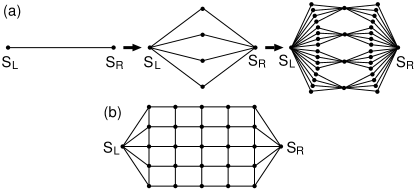
Figure 1: (a) The construction of the hierarchical lattice ($b=2$, $d=3$). (b) The lattice for the DWRG method in the EA SG.

DWRG method and observables— Let us first explain models for the DWRG method BrayMoore85 ; Hukushima99 ; Sasaki05 . Figure 1 (a) shows the way to construct the hierarchical lattice for the MK SG. The lattice is made iteratively by replacing each bond with $b^{d-1}$ paths, where $d$ is the dimension of the lattice. Each path consists of $b$ bonds, and new $(b-1)$ spins (full circles) are inserted in between. We hereafter call the two outermost spins ($S_{\rm L}$ and $S_{\rm R}$) boundary spins. The size $L$ of the lattice is multiplied by $b$ as the replacement is done once. Figure 1 (b) is the lattice for the EA SG. The lattice is the same as that in ref. Sasaki05 . It consists of two boundary spins and $L^{d}$ spins on a $d$-dimensional hyper-cubic lattice. The boundary condition is open in the direction along which the boundary spins lie, and is periodic in other directions. The Hamiltonian is

$${\cal H}=-\sum\nolimits_{\langle ij\rangle}J_{ij}S_{i}S_{j}-\sum\nolimits_{i}H_{i}S_{i},$$ (1)

where the first term is exchange energies between two nearest neighboring spins and the second term is Zeeman energies by field $H_{i}$.

In the DWRG method, we measure the effective coupling $J_{\rm eff}$ and the effective fields $H_{\rm eff}$ defined by

$$Z(S_{\rm L},S_{\rm R}) \equiv {\rm Tr^{\prime}}{\rm e}^{-H\{S\}/T}\propto{\rm e}^{{-\mathcal{H}}_{\rm eff}(S_{\rm L},S_{\rm R})/T},$$ (2)

$${\mathcal{H}}_{\rm eff}(S_{\rm L},S_{\rm R}) = -J_{\rm eff}S_{\rm L}S_{\rm R}-H_{\rm eff}^{\rm(L)}S_{\rm L}-H_{\rm eff}^{\rm(R)}S_{\rm R},$$ (3)

where the trace in Eq. (2) is for all the spins except $S_{\rm L}$ and $S_{\rm R}$. In the MK SG, $Z(S_{\rm L},S_{\rm R})$ is estimated exactly by taking the trace sequentially from the later generated spins to the earlier generated ones. For a detailed description of the procedure, we refer the reader to MiglioriniBerker98 . In the EA SG, on the other hand, probability $P(S_{\rm L},S_{\rm R})$ is measured by MC simulations Sasaki05 . Since $J_{\rm eff}$ and the free-energy difference $\delta F$ caused by twisting the two boundary spins are related by $J_{\rm eff}=-\delta F/2$ in zero field, we consider that $J_{\rm eff}$ represents the strength of the SG order. Because $J_{\rm eff}$ is either positive or negative, we calculate the standard deviation of sample-to-sample fluctuations of effective couplings, $\sigma_{\rm J}(L,H)$. We also measure that of effective fields $\sigma_{\rm H}(L,H)$. The correlation between effective couplings in zero field and those in field $H$ is also estimated by the correlation coefficient

$$C(L,H)=\frac{\overline{J_{\rm eff}(L,H)J_{\rm eff}(L,0)}}{\sigma_{\rm J}(L,H)\sigma_{\rm J}(L,0)},$$ (4)

where $\overline{\cdots}$ is the sample average. Here $J_{\rm eff}(L,H)$ and $J_{\rm eff}(L,0)$ are calculated for the same realization of $\{J_{ij}\}$.

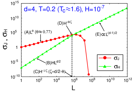
Figure 2: Size dependences of $\sigma_{\rm J}$ and $\sigma_{\rm H}$ in the four dimensional MK SG at $T\approx 0.125T_{\rm c}$, where $T_{\rm c}$ is the critical temperature in zero field. Strength of random fields is $10^{-7}$. (A) Size dependence of $\sigma_{\rm J}$ for smaller $L$. (B) Size dependence of $\sigma_{\rm H}$ for smaller $L$. (C) The size where the crossover between $\sigma_{\rm J}$ and $\sigma_{\rm H}$ occurs. (D) The value of $\sigma_{\rm J}$ and $\sigma_{\rm H}$ at the crossing point. (E) Size dependence of $\sigma_{\rm H}$ for larger $L$.

Results in the MK SG— Figure 2 shows the size dependences of $\sigma_{\rm J}$ and $\sigma_{\rm H}$ in the four-dimensional MK SG. The values of couplings $\{J_{ij}\}$ are taken from a Gaussian distribution of mean $0$ and width $1$. We apply random fields $H_{i}$ of strength $H$ by following the way in ref. MiglioriniBerker98 . The pool method BanavarBray87 is used to access huge sizes such as $L\approx 10^{10}$. The Zeeman energy $(\sigma_{\rm H}\propto HL^{d/2})$ overwhelms the effective coupling $(\sigma_{\rm J}\propto L^{\theta})$ around $L\approx H^{-1/\zeta}$, i.e., around the crossover length $\ell_{\rm cr}(H)$ in the droplet theory. After the crossing, $\sigma_{\rm J}$ exhibits roughly exponential decay and the exponent of $\sigma_{\rm H}$ changes from $d/2$ to $(d-1)/2$. These observations naturally lead us to the idea that $H^{\theta/\zeta}\sigma_{\rm J}$, $H^{\theta/\zeta}\sigma_{\rm H}$ and $C$ are scaled as functions of $X\equiv LH^{1/\zeta}$ which we call the scaling variable. The idea is tested in Fig. 3. The data with different $H$ and $L$ nicely collapse into scaling curves. These results clearly show the existence of the crossover length $\ell_{\rm cr}(H)$.

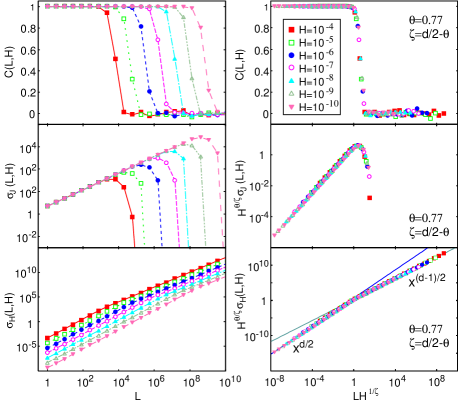
Figure 3: Raw data (left panel) and their scaling plots (right panel) in the MK SG. The dimensions and the temperature are the same as those in Fig. 2. The value $\theta=0.77$ obtained in ref. NifleHilhorst93 is used for the scaling. The two straight lines in the right-bottom panel are proportional to $x^{d/2}$ and $x^{(d-1)/2}$, respectively.

Results in the EA SG— Let us first explain some details of our simulation. The values of $J_{ij}$ are either $+J$ or $-J$ with equal weights. Uniform field $H$ is applied to all the spins except $S_{\rm L}$ and $S_{\rm R}$. The number of samples is more than $1,500$ for all the sets of $(L,H)$. We use the exchange MC method HukushimaNemoto96 to accelerate the equilibration, and the method in ref. Hukushima99 to overcome a hard-relaxing problem of the boundary spins which is originated from their high connectivities. The temperature ranges used for the exchange MC are $0.5J\leq T\leq 4.0J$ ($T_{\rm c}\approx 1.1J$ Katzgraber06 ) for $d=3$ and $1.0J\leq T\leq 4.5J$ ($T_{\rm c}\approx 2.0J$ MarinariZuliani99 ) for $d=4$. We hereafter focus on the data at the lowest temperature which is well below $T_{\rm c}$. We set the MC step for thermalization and that for measurement to be equal. They are sufficiently (at least 5 times) larger than the ergodic time to ensure the equilibration, where the ergodic time is the average MC step for a specific replica to move from the lowest to the highest temperature and return to the lowest one. As done in ref. Hukushima99 , we have also checked that MC runs starting from parallel and anti-parallel boundary spins yield identical results within error bars.

Figures 4 and 5 show the results for $d=3$ and those for $d=4$, respectively. Since $C$ is a dimensionless quantity, it is a function of only $X=LH^{1/\zeta}$. We therefore estimate $\zeta$ by fitting the data of $C$. By assuming the scaling relation $\zeta=d/2-\theta$ predicted by the droplet theory, $\theta$ is estimated to be $0.29(3)$ for $d=3$ and $0.60(2)$ for $d=4$. Since they are close to both recent estimations by Boettcher Boettcher04 (0.24(1) for $d=3$ and 0.61(2) for $d=4$) and direct estimations by linear least-square fits of $\ln[\sigma_{\rm J}(L,H=0)]$ against $\ln(L)$ (0.28(3) for $d=3$ and 0.69(3) for $d=4$), our data support the scaling relation.

We next examine scaling properties of $\sigma_{\rm J}$ and $\sigma_{\rm H}$ by using the values of $\theta$ determined above. The scaling reasonably works except $\sigma_{\rm J}$ for $d=4$. The deviation suggests that the fields investigated are too large or/and the sizes are too small so that corrections to the scaling is not negligible. In fact, if we closely observe the scaling plot of $\sigma_{\rm J}$ for $d=3$, we notice that the data with large $H$, say $H\geq 0.48$, systematically deviate from the master curve, while the data with small field are scaled quite well. If we estimate $\theta$ by forcing all the data to be scaled approximately, we get apparently larger values of $\theta$ in both $\sigma_{\rm J}$ and $\sigma_{\rm H}$. For example, $\theta$ estimated from $\sigma_{\rm J}$ in such way is $0.36\pm 0.02$ for $d=3$ and $0.84\pm 0.04$ for $d=4$.

The crossover behavior in the MK SG shown in Fig. 3 look very sharp in comparison with that in the EA SG. This is simply because the ranges of $H$ and $L$, and so $X$, are quite wide. The enlargement of the crossover region such as to $0.1\ \raise 1.29167pt\hbox{$<$}\kern-8.00003pt\lower 3.01385pt\hbox{$\sim$}\ X\ \raise 1.29167pt\hbox{$<$}\kern-8.00003pt\lower 3.01385pt\hbox{$\sim$}\ 10$ is realized by choosing the parameter ranges, for example, $0.015J\leq H\leq 0.95J$ and $L=3^{n}$ with $1\leq n\leq 4$. These ranges are close to those we are forced to choose for the EA SG. We then obtain quite similar results (not shown) as those obtained in the EA SG (Fig. 4). Within these ranges $\sigma_{\rm J}$ increases monotonically for smaller $H$ and it decreases monotonically for larger $H$. Still, such data are reasonably scaled with the same value of $\theta$ as indicated in Fig. 3. These observations imply that the observed scaling behaviors in both the MK and EA SGs are essentially the same.

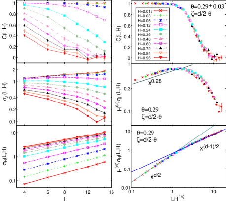
Figure 4: Raw data (left panel) and their scaling plots (right panel) in the EA SG at $T=0.5J$ for $d=3$. The value of $\theta$ is estimated by fitting the data of $C$, and the value is used for the scaling plot of $\sigma_{\rm J}$ and that of $\sigma_{\rm H}$. The slope of the line in the right-middle panel is obtained by linear least-square fits of $\ln[\sigma_{\rm J}(L,H=0)]$ against $\ln(L)$.

Interpretation of results— We first consider the crossover behavior in $\sigma_{\rm H}$. Since the field is not applied to the boundary spins, the effective fields $H_{\rm eff}^{\rm(L)}$ and $H_{\rm eff}^{\rm(R)}$ originate only through the influence of the field applied to the bulk spins $\{S_{i}\}$. For example, if the correlation between $S_{i}$ and $S_{\rm L}$ is positive, an upward field to $S_{i}$ tends to direct $S_{\rm L}$ upwards. Since the correlation can be either positive or negative depending on the site, the contribution to the effective fields can also be either positive or negative. When the effective coupling $J_{\rm eff}$ exists, $S_{\rm L}$ and $S_{\rm R}$ receive such random contributions, whose amplitude is proportional to $H$, from all the bulk spins. This yields $\sigma_{\rm H}$ which is proportional to $HL^{d/2}$. When $J_{\rm eff}$ vanishes, on the other hand, $\sigma_{\rm H}\propto L^{(d-1)/2}$ because the boundary spins, which interact with $L^{d-1}$ spins, receive contributions only from spins around their surfaces.

Now the meaning of our results are clear. As shown in Fig. 2, the Zeeman energy ($\sigma_{\rm H}$) begins to overwhelm the effective coupling ($\sigma_{\rm J}$) around $L\approx\ell_{\rm cr}(H)$ since $\sigma_{\rm H}$ increases faster than $\sigma_{\rm J}$. After that, $\sigma_{\rm J}$ rapidly drops to zero. This means that the SG order whose length scale is longer than $\ell_{\rm cr}(H)$ is destroyed by field. As described above, $\sigma_{\rm H}$ is kept increasing but with the change of its exponent from $d/2$ to $(d-1)/2$. The decay of $C(L,H)$ to zero for larger scaling variable $X$ indicates the vanishing of the correlation between the state in zero field and that in field. The observed scaling behavior consistently implies the absence of the SG phase in any non-zero field.

Discussion and conclusions— Now let us argue on the fragility of the SG state against other perturbations. According to the droplet theory, a change in the temperature (or bonds) by the amount $\Delta$ gives rise to a new SG state which is decorrelated to the original one beyond the length scale $\ell_{\rm ch}(\Delta)$. Here $\ell_{\rm ch}(\Delta)$ is proportional to $\Delta^{-1/\zeta^{*}}$ with $\zeta^{*}\equiv d_{\rm s}/2-\theta$, $d_{\rm s}$ being the fractal dimension of droplets. This type of the fragility of the SG state is called temperature or bond chaos BrayMoore87 . Our recent DWRG study Sasaki05 in the EA SG has indeed revealed the existence of $\ell_{\rm ch}(\Delta)$. A key observable in such studies is the correlation coefficient $C$ of Eq. (4) with $H$ replaced by $\Delta$. As shown in Figs. 3, 4 and 5, the system exhibits similar fragility against the field perturbation. However, it must be noted that vanishing of $\sigma_{\rm J}$ for larger $X$ strongly indicates that the magnetic field destroys the SG order itself in sharp contrast to the cases of temperature and bond perturbations.

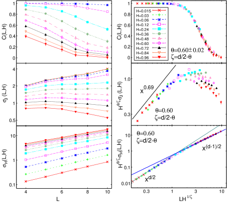
Figure 5: The same plot as that in Fig. 4 for the four dimensional EA SG at $T=1.0J$.

To conclude, we have studied the EA SG in field by a numerical DWRG method. The thermodynamic observables of the EA SG are confirmed to follow the scaling in terms of the crossover length $\ell_{\rm cr}(H)$ as predicted by the droplet theory, the consequence of which is the absence of the SG phase in field. It should be noted that above the upper critical dimension $d_{\rm u}=6$ different scenario may hold KatzgraberYoung05 . We consider that all of our results concerning the temperature, bond and field perturbations provide us a strong evidence for the appropriateness of the droplet theory for the description of SGs in low dimensions.

Acknowledgments— This work is supported by Grant-in-Aid for Scientific Research Program (#18740226 and #18079004) from MEXT in Japan. The computation in this work has been done using the facilities of the Supercomputer Center, Institute for Solid State Physics, University of Tokyo.

References

- (1) J. R. L. de Almeida and D. J. Thouless, J. Phys. A 11, 983 (1978).
- (2) D. S. Fisher and D. A. Huse, Phys. Rev. B 38, 386 (1988).
- (3) A. J. Bray and M. A. Moore, J. Phys. C 17, L613 (1984).
- (4) A. J. Bray and M. A. Moore, in Heidelberg Colloquium on Glassy Dynamics, Lecture Notes in Physics 275, (Springer, Berlin, 1987).
- (5) H. A. Katori and A. Ito, J. Phys. Soc. Jpn. 63, 3122 (1994).
- (6) J. Mattsson et al., Phys. Rev. Lett. 74, 4305 (1995).
- (7) P. E. Jönsson et al., Phys. Rev. B 71, 180412(R) (2005)
- (8) S. F. Edwards and P. W. Anderson, J. Phys. F 5, 965 (1975).
- (9) E. Marinari et al., J. Phys. A 31, 6355 (1998).
- (10) F. Krzakala et al., Phys. Rev. Lett. 87, 197204 (2001).
- (11) J. Houdayer and O. C. Martin, Phys. Rev. Lett. 82, 4934 (1999).
- (12) H. Takayama and K. Hukushima, J. Phys. Soc. Jpn. 73, 2077 (2004); J. Phys. Soc. Jpn. 76, 013702 (2007).
- (13) A. P. Young and H. G. Katzgraber, Phys. Rev. Lett. 93, 207203 (2004).
- (14) M. Sasaki et al., Phys. Rev. Lett. 95, 267203 (2005).
- (15) G. Migliorini and A. N. Berker, Phys. Rev. B 57, 426 (1998).
- (16) A. J. Bray and M. A. Moore, Phys. Rev. B 31, 631 (1985).
- (17) K. Hukushima, Phys. Rev. E 60, 3606 (1999).
- (18) J. R. Banavar and A. J. Bray, Phys. Rev. B 35, 8888 (1987).
- (19) M. Ney-Nifle and H. J. Hilhorst, Physica A 193, 48 (1993).
- (20) K. Hukushima and K. Nemoto, J. Phys. Soc. Jpn. 65, 1604 (1996).
- (21) H. G. Katzgraber et al., Phys. Rev. B 73, 224432 (2006).
- (22) E. Marinari and F. Zuliani, J. Phys. A 32, 7447 (1999).
- (23) S. Boettcher, Eur. Phys. J. B 38, 83 (2004).
- (24) A. J. Bray and M. A. Moore, Phys. Rev. Lett. 58, 57 (1987).
- (25) H. G. Katzgraber and A. P. Young, Phys. Rev. B 72, 184416 (2005).