Absence of skew scattering in two-dimensional systems:
Testing the origins of the anomalous Hall effect
Mario F. Borunda
Department of Physics, Texas A&M University,
College Station, TX 77843-4242, USA
Tamara S. Nunner
Institut für Theoretische Physik, Freie Universität Berlin, Arnimallee 14, 14195 Berlin, Germany
Thomas Lück
Institut für Theoretische Physik, Freie Universität Berlin, Arnimallee 14, 14195 Berlin, Germany
N. A. Sinitsyn
CNLS/CCS-3, Los Alamos National Laboratory, Los Alamos, NM 87545, USA
Department of Physics, Texas A&M University,
College Station, TX 77843-4242, USA
Carsten Timm
Department of Physics and Astronomy, University of Kansas, Lawrence, KS 66045, USA
J. Wunderlich
Hitachi Cambridge Laboratory, Cambridge CB3 0HE, UK
T. Jungwirth
Institute of Physics ASCR, Cukrovarnická 10, 162 53
Praha 6, Czech Republic
School of Physics and Astronomy, University of Nottingham,
Nottingham NG7 2RD, UK
A. H. MacDonald
Department of Physics, University of Texas at Austin,
Austin TX 78712-1081, USA
Jairo Sinova
Department of Physics, Texas A&M University,
College Station, TX 77843-4242, USA
(February 12, 2007)
Abstract
We study the anomalous Hall conductivity in spin-polarized, asymmetrically
confined two-dimensional electron and hole systems, focusing on skew-scattering
contributions to the transport. We find that the skew scattering,
principally responsible for the extrinsic contribution to the anomalous Hall
effect, vanishes for the two-dimensional electron system if both chiral Rashba
subbands are partially occupied, and vanishes always for the two-dimensional
hole gas studied here, regardless of the band filling. Our prediction can be
tested with the proposed coplanar two-dimensional electron/hole gas device and
can be used as a benchmark to understand the crossover from the intrisic to
the extrinsic anomalous Hall effect.
pacs:
72.15.Eb,72.20.Dp,72.25.-b
Introduction.—The observed Hall resistance of a magnetic film
contains the ordinary Hall response to the external magnetic field and the
anomalous Hall response to the internal magnetization. Although the anomalous
Hall effect (AHE) has been used for decades as a basic characterization tool
for ferromagnets, its origin is still being debated, also in the context of a
closely related novel phenomenon, the spin Hall effect
SHEtheory ; Kato:2004_d ; Wunderlich:2004_a ; Sih:2005_a . Three mechanisms
giving rise to AHE conductivity have been identified: (1) an intrinsic
mechanism based solely on the topological properties of the Bloch states
originating from the spin-orbit-coupled electronic structure
Karplus:1954_a , (2) a skew-scattering mechanism originating from the
asymmetry of the scattering rate Smit:1955_a , and (3) a side-jump
contribution, which semiclassically is viewed as a side-step-type of
scattering and contributes to a net current perpendicular to the initial
momentum Berger:1970_a .
Recent experimental and theoretical studies of transition-metal
ferromagnets and of less conventional systems, such as diluted magnetic
semiconductors, oxide and spinel ferromagnets, etc., have collected numerous
examples of the intrinsic AHE and of the transition to the extrinsic AHE
dominated by disorder scattering AHEmultiple . The unambiguous
determination of the origin of the AHE in these experimental systems is
hindered, in part, by their complex band structures, which has motivated
studies of simpler model Hamiltonians, such as the two-dimensional (2D) Rashba
and Dirac band models Dugaev et al. (2005); Sinitsyn et al. (2005); Liu and Lei (2005); ichiro Inoue et al. (2006); Onoda et al. (2006). Attempts to describe
all the contributions to the AHE within the same framework have yielded
farraginous results, however. So far a rigorous connection of the more
intuitive semiclassical transport treatment with the more systematic
diagramatic treatment, providing a clear-cut interpretation of the intrinsic,
skew, and side-jump AHE terms, has only been demonstrated for the Dirac
Hamiltonian model Sinitsyn et al. (2006).
In this Letter we calculate the transport coefficients in these two
complementary approaches for asymmetrically confined 2D electron and hole gases
in the presence of spin-independent disorder, finding perfect agreement. The
motivation for the study of these systems is threefold: First, they can be
represented by simple spin-orbit-coupled bands, which, similar to the Dirac
Hamiltonian model, allows us to unambiguously identify the individual AHE
contributions. Second, the extrinsic skew-scattering term vanishes for a
two-subband occupation in the case of the Rashba 2D electron gas and for
any band occupation for the studied 2D hole gas. This provides a
clean test of the intrinsic AHE mechanism and of the transition between the
intrinsic and skew-scattering-dominated AHE. Finally, we propose a 2D
electron gas/2D hole gas coplanar magneto-optical device in which the unique
AHE phenomenology found in our theoretical models can be systematically
explored experimentally.
Model Hamiltonians.—We study the following 2D model Hamiltonians:
(1)
with being the effective in-plane mass, the
Pauli matrices, , the exchange field, the
spin-orbit coupling parameter, and a spin-independent disorder
potential. The exponent () describes a 2D electron (hole) gas
Winkler:2003 . The eigenenergies of the clean system are . The eigenvectors in the clean
system take the form with and
(2)
where . We now define as
the wave number for the band at a given energy and define
. If is not specified, it is assumed to be
the Fermi energy. We consider the model of randomly located -function
scatterers, with
random and disorder averages satisfying , , and . This model is
different from the standard white-noise disorder with , where is the impurity
concentration and other correlators are either zero or related to this
correlator by Wick’s theorem. The deviation from white noise in our model is
quantified by , and is necessary to capture part of the
skew-scattering contribution to the AHE.
Semiclassical approach.—We sketch here the semiclassical procedure
used in the calculation, for further details we refer to Ref. Sinitsyn et al., 2006. The multi-band Boltzmann equation in a weak
electric field is given by
(3)
where ), is the subband index, and
is the impurity collision integral. The
distribution function is the sum of the equilibrium function and a
correction, . The scattering rates are
related to the T-matrix elements through where , and are eigenstates of
the complete Hamiltonian, and
of the disorder-free Hamiltonian.
Skew scattering.—Skew scattering appears in the Boltzmann equation
through the asymmetric part of the scattering rate, i.e., Smit:1955_a . The scattering rates to second and third
order in disorder strength are given by
where
is symmetric. Here . We break up the third-order contribution into
symmetric and antisymmetric parts. We ignore the first, since only the second
gives rise to skew scattering. This antisymmetric term is given by
Sinitsyn et al. (2006)
(4)
The solution of the Boltzmann equation (3) is found by first
looking at the deviation of the distribution function from equilibrium
Sinitsyn et al. (2006),
(5)
Assuming that the transverse conductivity is much smaller than the longitudinal
one () and substituting Eq. (5) into
Eq. (3) one finds and , where
(6)
(7)
For symmetric Fermi surfaces, the skew-scattering contribution to the conductivity
tensor at zero temperature can now be expressed using the scattering times,
(8)
The calculation of and uses the
matrix elements of Eq. (4). To simplify the notation we define
(9)
where all momenta are taken on the Fermi surface. Note that in Eq. (9)
the magnitude of can be different from that of or since
the Fermi momenta of different bands do not coincide.
The matrix elements appearing in Eq. (9) can be calculated directly from
the basis functions, yielding
(10)
from which we obtain
(11)
where is related to the density of states of each band at the Fermi
energy, . The symmetric part of the scattering rates to second order
in the disorder potential is given by The relaxation times are found by
inserting this into Eq. (6) and Eq. (11) into
Eq. (7). For , i.e., for the 2D electron gas, the
relaxation rates are then
(12)
(13)
where . If both subbands are occupied, the last factor in
Eq. (13) vanishes and there is no skew-scattering contribution. If
only the majority subband is occupied (), is
non-zero and skew scattering contributes. For the skew-scattering Hall
conductivity and the longitudinal conductivity we obtain in this case
(14)
(15)
If , i.e., for the 2D hole gas, we obtain
(16)
(17)
and skew scattering vanishes irrespective of band filling.
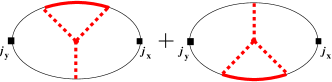
Figure 1: (color online).
Diagramatic representation of the skew-scattering contribution to
. Both current vertices, denoted by squares, are renormalized
by ladder vertex corrections.
Microscopic approach.—Within the diagramatic
Kubo formalism the skew-scattering contribution to the
off-diagonal conductivity is obtained from the expression
(18)
where the bare velocity vertex factors in the linear-in- Rashba
model are given by
(19)
As shown in a previous study Sinitsyn et al. (2006), the skew-scattering
contribution proportional to corresponds to the diagrams
shown in Fig. 1, where the current vertices on both
sides are the bare velocities renormalized by ladder vertex
corrections. Only the skew-scattering diagrams with a single
third-order vertex, shown in Fig. 1, contribute to order
. All other terms from a ladder-type summation of
third-order vertices are smaller because they are either not of the order
or of higher order in . The sum of the skew-scattering
vertices (i.e., the bold/red part of Fig. 1) gives
(20)
In the linear Rashba model we find , implying
that skew scattering vanishes if both subbands are occupied. In the case that
only one subband is occupied the evaluation of Fig. 1 to order
yields exactly the same expression for as in the semiclassical Eq. (15). The only effect of the
ladder vertex corrections is to renormalize each bare velocity by a factor of
which reduces to a factor of in the
limit of small and to a factor of in the limit of small .
For the 2D hole-gas model Hamiltonian (1) with
the bare velocity vertex factors are
(21)
Here the vertex corrections disappear because integrals of the type vanish. This implies the absence of skew scattering for
any subband filling Bernevig and Zhang (2005), consistent with the semiclassical
result. We note that the same consistency between semiclassical and microscopic
quantum theory calculations for the studied 2D models is also obtained for the
intrinsic and side-jump terms similar to the results in the graphene model
Sinitsyn et al. (2006); the longer details of those calculations will be shown
elsewhere and are in general agreement with Ref.
ichiro Inoue et al., 2006.
The abscence of the skew scattering is akin but not equivalent to the results
of spin-Hall-effect calculations in 2D systems Inoue et al. (2004). For the
Rashba 2D electron gas the disappearance of the DC spin Hall conductivity is
guaranteed by sum rules that relate the spin current to the dynamics of the
induced spin polarization Burkov:2004_a ; Chalaev and Loss (2004). In the case of
a charge current no similar sum rule is known. As we have shown, the
skew-scattering contribution in fact becomes finite when the minority band is
depleated. The vanishing of the Hall conductivity in the Rashba 2D electron
gas for is attributed to the simplicity of the Hamiltonian. In
particular the relation does not hold
generally beyond the case of the linear-in- Rashba coupling. The
abscence of skew scattering in the 2D hole system has a different origin: Due
to the cubic dependence of spin-orbit coupling on momentum, the matrix
elements, Eq. (10), in the antisymmetric part of the collision term
behave like . Together with the
dependence of the velocity factor in Eq. (7), this makes the
integral over vanish.
Our results predict that the AHE in 2D electron and hole systems can be
dominated by contributions independent of the impurity concentration, for which
the anomalous Hall resistance is . We also predict
that in the Rashba 2D electron gas with only one subband occupied the extrinsic
skew-scattering contribution, leading to anomalous Hall resistance proportional
to , is non-zero. Note that this term has not been
identified in previous works that considered only white-noise disorder
Dugaev et al. (2005); Sinitsyn et al. (2005); Liu and Lei (2005); ichiro Inoue et al. (2006); Onoda et al. (2006).
Since its corresponding conductivity contribution is inversely proportional to
the impurity concentration, the skew-scattering mechanism can dominate in
clean samples.
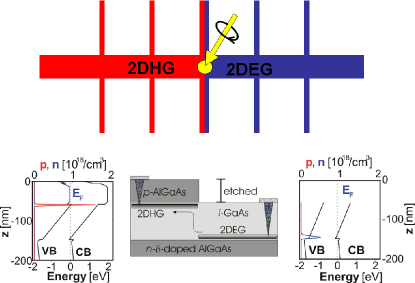
Figure 2: (color online). Top panel: Top-view schematics of the Hall bar with
coplanar 2D hole and electron gases. Spin-polarized carriers are generated by
shining circularly polarized light on the p-n junction. Center bottom panel:
Cross section of the heterostructure containing p-type and n-type AlGaAs/GaAs
single junctions. The left band diagram corresponds to the unetched part of the
wafer with the 2D hole gas, the right band diagram shows the 2D electron gas in
the etched section of the wafer.
Proposed experimental setup.—The unique phenomenology of
the AHE in the studied 2D systems, in particular the sudden disappearance of
skew scattering when the Fermi level crosses the depletion point of the
minority 2D Rashba band, represents an opportunity for a clean test of the
presence of intrinsic and extrinsic sources of the AHE and of the transition
between these two regimes. In the absence of 2D ferromagnetic system with
Rashba like spin-orbit interatciton, we proposed an experimental setup for this
test as shown in Fig. 2. The device is based on a AlGaAs/GaAs
heterostructure containing a coplanar 2D hole gas/2D electron gas p-n junction.
The cross section of the heterostructure and corresponding band diagrams are
shown in the lower panels of Fig. 2 (for more details see
Ref. Wunderlich:2004_a, ). Under a forward bias the junction was
successfully utilized as a light-emitting-diode spin detector for the spin Hall
effect Wunderlich:2004_a . Here we propose to operate the junction in the
reverse-bias mode, while shining monochromatic, circularly polarized light of
tuneable wavelength on the p-n junction. The photogenerated spin-polarized
holes and electrons will propagate in opposite directions through the
respective 2D hole and electron channels. The longitudinal voltage and the
generated anomalous Hall voltage can be detected by the successive sets of Hall
probes, as shown in the upper panel of Fig. 2. For the 2D
electron gas the macroscopic spin diffusion length allows to use standard
lithography for defining the Hall probes. Surface or back gates in close
proximity to the 2D electron system can be used to modify the effective 2D
confinements, carrier density, and spin-orbit coupling in order to control the
transition between the intrinsic and extrinsic AHE regimes. The exploration of
the AHE in the 2D hole gas is more challenging due to the expected sub-micron
spin diffusion length in this system but may still be feasible in the proposed
experimental setup.
Acknowledgements.
Fruitful discussions with S. Onoda and N. Nagaosa are gratefully
acknowledged. This work was supported by ONR under Grant No. ONR-N000140610122, by the NSF under Grants No. DMR-0547875 and No. PHY99-07949, by the SRC-NRI (SWAN), by EU Grant IST-015728, by EPSRC Grant
GR/S81407/01, by GACR and AVCR Grants 202/05/0575, FON/06/E002, AV0Z1010052,
and LC510, by the DOE under Grant No. DE-AC52-06NA25396, and by the Univ. of
Kansas General Research Fund allocation No. 2302015. Jairo Sinova is a
Cottrell Scholar of Research Corporation.
References
(1)
M. I. Dyakonov
and V. I. Perel,
JETP 467 (1971);
S. Murakami,
N. Nagaosa, and
S.-C. Zhang,
Science 301,
1348 (2003);
J. Sinova et al.,
Phys. Rev. Lett. 92,
126603 (2004).
(2)
Y. K. Kato et al.,
Science 306,
1910 (2004).
(3)
J. Wunderlich et al.,
Phys. Rev. Lett. 94,
047204 (2005).
(4)
V. Sih et al.,
Nature Physics 1,
31 (2005).
(5)
R. Karplus and
J. M. Luttinger,
Phys. Rev. 95,
1154 (1954).
(6)
J. Smit,
Physica 21, 877
(1955).
(7)
L. Berger, Phys. Rev.
B 2, 4559 (1970).
(8)
J. Banhart and
H. Ebert,
Europhys. Lett. 32,
517 (1995);
J. Ye et al.,
Phys. Rev. Lett. 83,
3737 (1999);
T. Jungwirth,
Q. Niu, and
A. H. MacDonald, ibid.88, 207208 (2002);
Y. Yao et al., ibid.92, 037204 (2004);
Y. Taguchi et al.,
Science 291, 5513
(2001);
W.-L. Lee et al., ibid.303, 1647 (2004);
J. Kötzler and
W. Gil, Phys. Rev.
B 72, 060412(R) (2005);
B. C. Sales et al., ibid. 73, 224435 (2006);
C. Zeng et al.,
Phys. Rev. Lett. 96,
037204 (2006);
S. H. Chun et al.,
ibid.98, 026601 (2007);
J. Cumings et al., ibid.96, 196404 (2006);
T. Miyasato et al.,
eprint cond-mat/0610324.
Dugaev et al. (2005)
V. K. Dugaev et al.,
Phys. Rev. B 71,
224423 (2005).
Sinitsyn et al. (2005)
N. A. Sinitsyn et al.,
Phys. Rev. B 72,
045346 (2005).
Liu and Lei (2005)
S. Y. Liu and
X. L. Lei,
Phys. Rev. B 72,
195329 (2005).
ichiro Inoue et al. (2006)
J. Inoue et al.,
Phys. Rev. Lett.
97, 046604
(2006).
Onoda et al. (2006)
S. Onoda,
N. Sugimoto, and
N. Nagaosa,
Phys. Rev. Lett. 97, 126602 (2006).
Sinitsyn et al. (2006)
N. A. Sinitsyn et al.,
Phys. Rev. B 75, 045315 (2007).
(15) R. Winkler, Spin-Orbit Coupling Effects in Two-
Dimensional Electron and Hole Systems, Springer Tracts in Modern Physics, vol. 191 (Springer,
Berlin, 2003).
Bernevig and Zhang (2005)
B. A. Bernevig and
S.-C. Zhang,
Phys. Rev. Lett. 95,
016801 (2005).
Inoue et al. (2004)
J. Inoue,
G. E. W. Bauer,
and L. W.
Molenkamp, Phys. Rev.
B 70, 041303
(2004), eprint cond-mat/0402442.
(18)
A. A. Burkov,
A. S. Nuñez, and
A. H. MacDonald,
Phys. Rev. B 70,
155308 (2004).
Chalaev and Loss (2004)
O. Chalaev and
D. Loss,
Phys. Rev. B 71,
245318 (2004).