String excitations of a hole in a quantum antiferromagnet and photoelectron spectroscopy

Abstract

The aim of the present paper is twofold. The first goal is to show that high resolution angle-resolved photoelectron spectra from cuprates indicate the presence of string-like excitations of the quasihole excitation in a quantum antiferromagnet. In order to compare with the experimental intensity plots, we calculate the spectral function of the $t-J$ and the $t-t^{\prime}-t^{\prime\prime}-J$ models within the self-consistent Born approximation for widely accepted values of the parameters of these models. The main features of the high resolution photoelectron spectra are in general agreement with the results based on the above models and can be understood by considering not only the lowest energy quasiparticle peak but, also, the higher energy string-like excitations of the hole. These features are: (a) the energy-momentum dispersion of the string-like excitations, (b) the momentum dependence of the spectral weight of the quasiparticle peak, and (c) the way in which the spectral weight of the lowest energy quasiparticle peak is transfered to higher energy string excitations, including the fact that it vanishes near the $\Gamma$ point. The second goal of the present paper is to make the case that a proper analysis of both the numerical results obtained from these models and of the experimental results, suggests a theoretical picture for the internal structure of the hole-quasiparticle and a string-exchange pairing mechanism due to strong antiferromagnetic correlations among the background spins. We find that, using a simple model in which the Hilbert space is restricted to states of only unbroken strings attached to the holes and in which the holes are connected with unbroken strings, we can provide a good quantitative description of the most accurate numerical results. We find that the holes experience an effective interaction due to a string-exchange mechanism which is characterized by a rather large string tension and this can provide pairing energy scales much larger that those suggested by spin-fluctuation mediated pairing models. In addition, it is argued that such string-exchange interaction tends to bind holes in a bound state with the $d_{x^{2}-y^{2}}$ symmetry.

I Introduction

Angle-resolved photoelectron spectroscopy (ARPES) studies of the cuprates and related materials have been very useful in revealing the structure of the low energy quasiparticle excitationswells ; damascelli ; ronning ; graf . In this paper, we will focus on the most recent high resolution ARPES studiesronning ; graf where an “anomalous” dispersion was identified at relatively higher energy than the well-known low energy quasiparticle band in the under-doped regime. We would like to discuss the case of very light doping where there are concrete predictions for the hole spectral function in a quantum antiferromagnetliu ; dagottor . In this limit the problem has been extensively studied and from that ground and the above mentioned experimental studies a novel physical picture emerges which consists of some already known features and some new ideas to be discussed here.

The motion of a single hole inside a quantum antiferromagnet has been extensively studied using a number of analytical, semi-analytical and numerical techniques. One of the main and well-known conclusions of these studies is that the hole becomes a rather well-defined low-energy quasiparticle with the minimum of the quasiparticle band at $(\pm\pi/2,\pm\pi/2)$, which is an unusual position in the Brillouin zone for a minimum to occur, and, thus, at sufficiently light doping, a hole pocket develops near $(\pm\pi/2,\pm\pi/2)$. In addition, quantum spin-fluctuations allow the hole to move coherently as a polaron because of the fact that they can erase the damage created by the hole and, vice versa, the hole through its motion which displaces reversed spins can eliminate some spin-deviations created in advance by quantum fluctuations; thus, the hole motion can lower the total energy because it repairs some damage by “choosing” to move through paths of already reversed spins. Angle-resolved photoelectron studies of the undoped insulator have demonstratedwells that the minimum of the hole band is at $(\pm\pi/2,\pm\pi/2)$ and the bandwidth is in very good agreement to that predicted from the $t-J$ modelliu when the experimentally determined valueRMP of $J\simeq 0.13eV$ and the empirically known value of $t\simeq 0.4eV$ are used. The dispersion along the direction $(0,0)$ to $(\pi,\pi)$ as calculated using the $t-J$ modelliu does not agree with that measured by ARPESwells and it requires an extension of the $t-J$ model to add nearest neighbor ($t^{\prime}$) and next nearest neighbor ($t^{\prime\prime}$) hopping to reproduce the experimental findings along this directionkim ; theory ; nazarenco ; ferrell ; lee ; wheatley ; belincher ; eder .

What is less well-known about the hole motion in a quantum antiferromagnet is what we call the string excitations which are internal excitations of the hole polaron. These excitations arise because the hole along its path creates a string of spins which are reversed relative to the local antiferromagnetically correlated background. These excitations have been discussed by Shraiman and Siggiashraiman0 ; shraiman1 ; shraiman2 and investigated further by several authorsbarnes ; dagotto ; elser ; liu . In particular in Ref. liu, , where a detailed calculation of the hole spectral function was reported, it was found that these excitations appear as rather sharp peaks in the hole spectral function and they compete with the low energy well-defined quasiparticle peak to gain spectral weight as a function of momentum.

The aim of the present paper is twofold. One of the goals of the present paper is to discuss that the recently reported high resolution angle resolved photoelectron studies from cupratesronning ; graf strongly indicate the existence of such string excitations in these materials (See also, Ref. manousakis, ). A possible connection between such string excitations and certain features of the spectral function was made in past experimental studiesronning ; kim . In the present paper, a detailed analysis of their possible role in the spectral function is provided along with a study of the consequences of their possible presence in doped quantum antiferromagnets. We provide a rather transparent physical picture, through which we can understand several features of the ARPES results in terms of the same unified framework. The analysis provided in the present paper, by recalculating the hole spectral function using the $t-J$ modelmanousakis and the $t-t^{\prime}-t^{\prime\prime}-J$ model in order to properly compare the results with the experimental data, makes a strong case for the existence of such string excitations in the real materials.

The second important goal of the present paper is to present a new framework to understand the possible role of local strong antiferromagnetic correlations in the doped cuprate materials in the pairing mechanism. First, we introduce a model based on a reduced Hilbert space which contains only unbroken strings of overturned spins attached to the holes. It is demonstrated that this reduced Hilbert space accurately captures the features of the quasiparticle dispersion and the higher energy string excitations. In addition, it is illustrated that using a subspace of states in which a pair of holes is connected with unbroken strings leads to a string-mediated interaction which might give significantly stronger pairing mechanism than models of pairing due to exchange of spin-fluctuations.

The paper is structured as follows: In Sec. II we present the results of the hole spectral function as calculated using the $t-J$ and the $t-t^{\prime}-t^{\prime\prime}-J$ models paying particular attention to the contribution and role of string excitations. In Sec. III, the analysis of the recent ARPES experimental results in order to reveal the contribution of the string excitations in the real materials is made. Sec. IV presents the consequences of our finding to our theoretical picture for the hole-quasiparticle in doped cuprates. In addition, a simple model is presented based on states of unbroken strings connected to the holes which gives a very good account of the numerical results of the $t-J$ model. In addition, a pairing mechanism through string exchange interaction is presented in the same section.

II Calculation of the spectral function

In this section of the paper we will use the same method used in Ref. liu, to calculate the spectral function of a hole in a quantum antiferromagnet using the $t-J$ and $t-t^{\prime}-t^{\prime\prime}-J$ models with the aim to make a direct comparison with the recent ARPES results.

In order to start the discussion, let us consider a quantum antiferromagnet doped with holes as described by the well-known $t-J$ model

$${\cal H} = -t\sum_{<ij>,\sigma}(c^{\dagger}_{i\sigma}c_{j\sigma}+c^{\dagger}_{i\sigma}c_{j\sigma})+J_{z}\sum_{<ij>}s^{z}_{i}s^{z}_{j}$$ (1)

$$+ {{J_{\perp}}\over 2}\sum_{<ij>}(s^{+}_{i}s^{-}_{j}+s^{-}_{i}s^{+}_{j})$$

which is restricted to operate in a single occupied subspace. Here $c^{\dagger}_{i\sigma}$ creates a spin $\sigma$ electron at lattice site $i$. The operators $s^{x,y,z}_{i}$ are the three components of a spin-1/2 operator and $s^{\pm}_{i}=s^{x}_{i}\pm is^{y}_{i}$. The first term takes into account the hole-hopping and the second and third are the direct and exchange terms in the Heisenberg antiferromagnet. Just the first two terms form a Hamiltonian known as the $t-J_{z}$ model. The $t-J$ model corresponds to the spacial case when $J_{z}=J_{\perp}$. The $t-t^{\prime}-t^{\prime\prime}-J$ model is obtained from the above $t-J$ model by adding a hopping term $t^{\prime}$ which allows the hole to move along the diagonal of the square lattice and a $t^{\prime\prime}$ term which moves the hole by two sites along the $\hat{x}$ direction (and $-\hat{x}$ direction) or by two sites along the $\hat{y}$ direction (and $-\hat{y}$ direction). The $t-t^{\prime}-t^{\prime\prime}-J$ model has been used in Refs. kim, ; theory, ; nazarenco, ; ferrell, ; lee, ; wheatley, ; belincher, ; eder, ; avinash, to rather successfully fit the photoemission data of Wells et al.wells

In Ref. liu, following Ref. KLR, an effective Hamiltonian was used where the Heisenberg spin interaction part of the $t-J$ model was treated in spin-wave approximation and the hole-hopping term was linearized in spin-deviation operators. Within the non-crossing approximation, the Dyson’s equation for the single-hole Green’s function was solved self-consistently. When the calculation was carried out on small-size lattices a very good agreement was found with the exact diagonalization results for the spectral function. However, the advantage of the method is that it can be carried out on sufficiently large size lattice where finite-size effects are entirely absentliu ; marsiglio ; martinez . Hence, we will use this method to calculate the hole spectral function for the $t-J$ and $t-t^{\prime}-t^{\prime\prime}-J$ models with the aim to make a direct comparison with the ARPES results.

Figure 1: The spectral function of a single hole in a quantum antiferromagnet for $J/t=0.3$ along the $(0,0)$ to $(\pi/2,\pi/2)$ direction as a function of energy $\omega$.

In Fig. 1 the hole spectral function is shown for the $t-J$ model along the $(0,0)$ to $(\pi/2,\pi/2)$ direction using the broadly accepted parameter values of $t=0.4eV$ and $J/t=0.3$. The Dyson’s equation was solved as in Ref. liu, using Lorentzian broadening with a width $\eta=0.1t$. We note that while the width of the first peak depends strongly on the value of $\eta$, as it is a $\delta$ function peak, the other two (labeled II and III) and the higher peaks (not clearly seen in the graph due to the choice of the scale) remain unchanged when we decrease the value of $\eta$. This point has been extensively studied in Ref. liu, and we have been able to reproduce it here. The first important point to be discussed in this paper again is the higher energy peaks labeled II and III in the spectral function. These peaks were studied in Ref. liu, and it was concluded that they correspond to the string-like excitations which can be understood in the simple $t-J_{z}$ model. Before we go on in this paper we wish to briefly discuss the origin of these peaks.

Let us first imagine a hole subject to quantum mechanics moving in a classical antiferromagnetic template such as the one conceptualized within the $t-J_{z}$ model. As the hole tries to move, it creates a string of spin deviations over the antiferromagnetic background and, thus, it experiences a linearly rising potentialshraiman0 ; shraiman1 . As a result, if we ignore the small probability amplitude for the hole to retrace its pathtrugman , the hole is bound to its “birth” site. In addition, there are excited statesbarnes ; dagotto ; liu of the hole inside the almost linearly rising potential which in the limit $t/J>>1$ can be approximated by the Airy functions and their corresponding eigenenergies are given by

$$E_{n}/t=\epsilon_{n}+a_{n}(J_{z}/t)^{2/3}.$$ (2)

Figure 2: (a) A hole, shown by an open circle, in an antiferromagnetically aligned background (the spins of the Néel background are not shown in this figure for clarity; only the spin-deviations are shown by a solid circle) with no spin-deviations. (b) The hole has moved along the shown path by displacing the spin and creating the spin deviations shown with the black dots and thus creating the string shown. (c) The pair-spin-flip term of the Heisenberg antiferromagnetic exchange can eliminate a pair of nearest-neighbor spin deviation at the beginning of the string and, thus, shortening the string or (d) in the middle of the string thereby cutting the string into a string with the hole at one end and just a string of spin-deviations.

Now, let us turn on the Heisenberg antiferromagnetic exchange coupling $J_{\perp}$. This term creates or eliminates nearest-neighbor pairs of spin-deviations and, thus, it makes it possible for the hole to become free of its original “birth” site and find its “umbilical-cord” attached to a new “birth” origin. As shown in Fig. 2 this can either happen by eliminating the pair of spin-deviation at the beginning of the string involving the “birth” location of the hole (Fig. 2(c) or anywhere along the string (Fig. 2(d), thus, producing two strings, one attached to the hole and the other becomes part of the background spin-deviations, i.e., part of the fluid of the spin-deviations which always exist in a quantum antiferromagnet due to zero temperature quantum fluctuations. In addition, to these processes there can be processes where the creation of pairs of spin-deviations adjacent to the hole position precedes the hole motion, in which case the hole experiences the string as a line of downhill potential. In the limit of $t/J_{\perp}>>1$, however, the spin-relaxation time is much longer that the characteristic time for hole-hopping. Thinking in the same spirit as the Born-Oppenheimer approximation for the electronic motion relative to the slowly moving ions, one can convince himself that the approximate notion of a linearly rising potential exists. The important difference from the simpler $t-J_{z}$ model is that these spin fluctuations, no matter how slow they maybe, play the leading role in delocalizing the “birth” site from where the string is attached. This process is the process which gives rise to the hole band with a minimum at $(\pi/2,\pi/2)$. We would like to stress, however, that a more correct qualitative picture is one where the hole is held by a string from a mobile birth-site. We will come back to this discussion in Sec. IV were we will examine further the role of these processes.

In Ref. liu, , the peaks II and III in Fig. 1, have been attributed to the internal excitations of the string analogous to the excitations of a particle in a linear potential. The energy where the peaks are located in the spectral function have been studied as a function of $J/t$ (in the $t-J$ model where $J_{\perp}=J_{z}=J$) and it was found that they fit to the form given by Eq. 2 with $J_{z}$ replaced by $J$ in a wide range of $J/t$. In addition, the width of these peaks was found to scale with $J/t$. In Sec. IV, the emergence of these peaks as higher energy excitations of the hole restricted in a Hilbert space of states made of only unbroken strings is discussed.

In the present paper, one of the important aspects of Fig. 1 that we notice is the vanishing of the spectral weight of the low energy quasiparticle peak as we move away from the minimum of the band at $(\pi/2,\pi/2)$ toward the $\Gamma$ (momentum $(0,0)$) point. In addition, notice that the spectral weight is transfered to the higher energy peaks which correspond to the string resonance excitations.

Figure 3: The spectral function of a single hole in a quantum antiferromagnet for the $t-t^{\prime}-t^{\prime\prime}-J$ model with the same parameter values used in Ref. kim, along the $(0,0)$ to $(\pi/2,\pi/2)$ direction as a function of energy $\omega$.

In Fig. 3 the calculated hole spectral function for the $t-t^{\prime}-t^{\prime\prime}-J$ model with the same parameter values used in Ref. kim, ($t=0.35eV$, $t^{\prime}=-0.12eV$, $t^{\prime\prime}=0.08eV$ and $J=0.14eV$) is shown along the $(0,0)$ to $(\pi/2,\pi/2)$ cut. Again, in this case also, the Dyson’s equation has been solved as in Ref. liu, using Lorentzian broadening with a width $\eta=0.1t$. This figure should be compared with Fig. 1 obtained for the pure $t-J$ model. All important aspects of the spectral function obtained with the simpler $t-J$ model remain the same. The only difference is that as we approach the $\Gamma$ point more spectral weight is transfered to the peak II instead of III.

Figure 4: The spectral function of a single hole in a quantum antiferromagnet for the $t-J$ model along the $(0,0)$ to $(\pi,0)$ direction as a function of energy $\omega$.

In Fig. 4 and Fig. 5, the calculated hole spectral function along the $(0,0)$ to $(\pi,0)$ cut is shown for the $t-J$ model and the $t-t^{\prime}-t^{\prime\prime}-J$ model respectively. The low energy quasiparticle excitation along this direction attains it minimum at $(\pi,0)$ in the $t-J$ model (Fig. 4) where the peak acquires most of the spectral weight. This is not the case in the experiment. As a result the $t-J$ model was extended to the $t-t^{\prime}-t^{\prime\prime}-J$ model precisely for this reason. Notice in Fig. 5 that the band minimum along this direction is no longer at $(\pi,0)$ but rather at $(\pi,/2,0)$ where the spectral weight in maximum. Again, notice that the spectral weight as we approach the $\Gamma$ point is transfered to the second peak due to the internal excitation of the string.

Figure 5: The spectral function of a single hole in a quantum antiferromagnet for the $t-t^{\prime}-t^{\prime\prime}-J$ model with the parameters used in Ref. kim, ($t=0.35eV$, $t^{\prime}=-0.12eV$, $t^{\prime\prime}=0.08eV$ and $J=0.14eV$) along the $(0,0)$ to $(\pi,0)$ direction as a function of energy $\omega$.

III Comparison with experiment

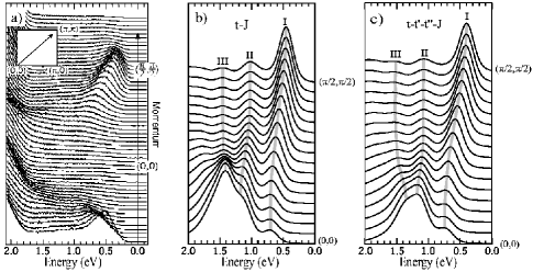
Figure 6: The experimentally determined spectral function with high resolution ARPESronning shown on the left (part a) is compared with the theoretical spectral functions obtained from the $t-J$ modelliu for $J/t=0.3$ and $t=0.4eV$ along the path from $(0,0)\to(\pi/2,\pi/2)$ shown in the middle (part b), and that obtained from the $t-t^{\prime}-t^{\prime\prime}-J$ model (part c) along the previously mentioned Brillouin Zone path. The solf-gray lines labeled I,II and III are guides to the eye. The reference energy has been shifted by a constant so that the energy of the quasiparticle peak at $(\pi/2,\pi/2)$ to be the same as the experiment.

The lowest energy peak at $(\pi/2,\pi/2)$ in the theoretical calculation is very sharp while in the experimental data it carries a width of the order of a fraction of an $eV$. It is not clear what is the exact mechanism which causes the damping of the quasiparticle and there are reasons to believe that it may be due to the coupling to phonon excitationsnagaosa . Therefore, in order to compare with the experimental results we need to broaden the results of our calculation. We use a Gaussian broadening function, namely $A_{b}({\bf k},\omega)=\int A({\bf k},\omega^{\prime})G(\omega-\omega^{\prime})d\omega^{\prime}$, where $G(\omega-\omega^{\prime})=exp(-(\omega-\omega^{\prime})^{2}/\epsilon^{2})$, using $\epsilon=\sqrt{2}\sigma=0.125eV$. We have obtained very similar results when we use a value of $\eta=0.125eV$ in the initial propagator namely in the iterative procedure to solve the Dyson’s equation. The same amount of broadening has been used in Ref. kim, to compare the ARPES peak to the quasiparticle peak given by the $t-t^{\prime}-t^{\prime\prime}-J$ model.

In Fig. 6 a comparison is presented between the experimental spectral function along the $(0,0)$ to $(\pi,\pi)$ cut, as reported in Ref. ronning, by means of high resolution ARPES (left or part (a)), and those obtained from the $t-J$ model (part (b)) and the $t-t^{\prime}-t^{\prime\prime}-J$ model (part (c)). We would like to notice that both in the theoretical and the experimental results, as we move away from $(\pi/2,\pi/2)$ toward $(0,0)$, the spectral weight of the low energy well-defined quasiparticle peak vanishes and it is gradually transfered to higher energy excitations. Notice that in the comparison of Fig. 6 and in the comparison provided in Fig. 7 and Fig. 8, if the energy scale of the theoretical results (i.e., the value of $t$) is increased by about $25\%$ (such that the theoretical peak at the $\Gamma$ point at $\sim 1.5eV$ is pushed to $\sim 2eV$) the agreement between theory and experiment becomes better, especially at higher energies near $2eV$. However, at such high energy scales we expect other effects to become important and the description, in terms of a Zhang-RiceZR singlet within the simple $t-J$ model, is also expected to fail.

In Fig. 7, we have produced an intensity plot along the $(0,0)$ to $(\pi,\pi)$ cut, in order to compare directly our results with those of Ref. ronning, . For the purpose of comparison, we have added the experimental results of Ref. ronning, as reported in their Fig. 2 (top of Fig. 7). In the second intensity plot from the top, we present that obtained from the $t-J$ model with the generally accepted parameter values mentioned earlier. The bottom intensity plot is that obtained from $t-t^{\prime}-t^{\prime\prime}-J$ model using the parameter values used in Ref. kim, . The intense peaks at $(\pi/2,\pi/2)$ and near $(0,0)$ are present in both theoretical and experimental intensity plots. As we approach momentum $(0,0)$ the spectral weight is transfered to higher energy “string” states (II and III) as also was discussed in Sec. II. This gradual transfer manifests itself as a more luminous path connecting the bright peaks at $(\pi/2,\pi/2)$ and $(0,0)$.

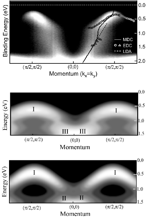
Figure 7: The experimentally observed intensity plot reported in Fig. 2 of Ref. ronning, (top) is compared with that obtained from the $t-J$ model (middle) and from the $t-t^{\prime}-t^{\prime\prime}-J$ model (bottom). The reference energy has been shifted by a constant so that the energy of the quasiparticle peak at $(\pi/2,\pi/2)$ to be the same as the experiment.

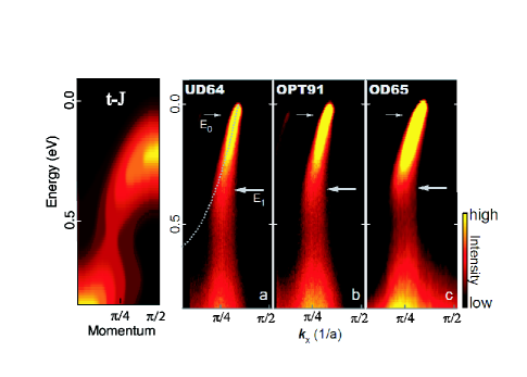
Figure 8: Left: The theoretical color coded intensity plot along the cut indicated in the top-right inset, as obtained from the $t-J$ model using the widely acceptable values for the parameters $J/t=0.3$ and $t=0.4eV$. Right: Three ARPES intensity plots for underdoped, optimally doped and overdoped $Bi2212$ taken from Fig. 1 of Ref. graf, for comparison.

In a very recent ARPES studygraf an anomalous dispersion was identified and a second energy scale at around $0.8eV$ was reported. In our calculation this energy scale is the average energy of the string excitation peaks II and III (measured from the lowest energy state at $(\pi/2,\pi/2)$). This becomes evident by comparing our Fig. 7 with Fig. 2 of Ref. graf, . In Fig. 8 we present a theoretical color-coded intensity plot (left) along the $(\pi/2,\pi/2)$ to $(0,0)$ cut, as obtained from the $t-J$ model to be compared with the three ARPES intensity plots (right part of Fig. 8) for underdoped, optimally doped and overdoped $Bi2212$ taken from in Fig. 1 of Ref. graf, . A very similar intensity plot was obtained for the case of the $t-t^{\prime}-t^{\prime\prime}-J$ model. First of all in making a comparison we must realize that the lowest energy quasiparticle states, which correspond to the lowest energy string states in the neighborhood of $(\pi/2,\pi/2)$, are occupied by holes which form a Fermi sea. Namely, these occupied states will be entirely dark in the intensity plot and the states with highest intensity would be right on the intersection of the Fermi surface with the most luminous states of the theoretical intensity plot. Therefore, by assuming these adjustments the color-coded intensity plot of Fig. 8, excluding the bright spots around $(\pi/2,\pi/2)$ (because at sufficient amount of doping the states around $(\pi/2,\pi/2)$ should be inside the Fermi sea and the bright spots should move just outside the Fermi surface), qualitatively agrees with the experimental intensity plots reported in Fig. 1 of Ref. graf, . These figures and the previous discussion clearly indicate that the process of spectral weight transfer to the higher string states is masked by low intensity and/or broadening and manifests itself in the intensity plot as an “anomalous” dispersion with the center of the anomaly close to $(\pi/4,\pi/4)$ as in Fig. 1 of Ref. graf, . We find it very interesting that these features persist all the way up to the overdoped regime. Our conclusion, therefore, is that the spin correlations should be strongly antiferromagnetic even in the overdoped cuprates and this point is discussed in the next section.

IV The string mediated interaction

IV.1 Role of string states in the single-hole dispersion

As we discussed the origin of the spectral function peaks is due to the string excitations and they provide a qualitative explanation of the vanishing of the spectral weight from the low energy quasiparticle peak by means of spectral weight shift to higher energy string excitations. In this part of the paper, motivated by these finding we will consider a new theoretical approach to understand doped quantum antiferromagnets, one in which such string excitations play a fundamental role.

First we notice that as the hole moves it does not simply create spin deviations, it creates (or destroys) a spatially connected string of spin-deviations. Therefore, as a basis to span the Hilbert space instead of disconnected spin-deviations we will consider an over-complete basis which is spanned by all possible strings which define connected paths of spin-deviations as shown in Fig. 2. The spin fluctuation part of our Hamiltonian conserves spin and creates or annihilates pairs of spin deviations which can be regarded as strings of two sites. The only case in which a single spin-deviation is needed is when we have a state where a spin-deviation is next to the site where the hole is located. This state can be regarded as a hole attached to a string of length unity.

The fundamental reason for the choice of this basis is that in the limit where $t>>J$, the quantum antiferromagnet with just a small hole concentration should look like a fluid of strings of overturn spins created by the motion of the holes with a lot of nearest-neighbor pairs of spin deviations (due to the spin conserving antiferromagnetic exchange) which can also be considered as strings of size two. In this regime, the average string size in the ground state should be larger than two. In addition, this basis describes better the short wavelength physics and it might provide a better description in the doped regime when the long-range spin correlations are destroyed, but the relatively short-range antiferromagnetic correlations are still present.

Figure 9: Connected single-hole string states up to length 4. The hole is represented by the open circle and the filled circle stands for a spin deviation. (a) The hole in the Néel background. (b) There are 4 states of string length unity. (c) There are 12 states of string length 2. (d) 36 states having string length 3 exist. (e) There are 108 states such the ones shown in Fig. (e) above with strings of length 4.

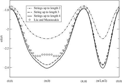
Figure 10: The hole dispersion as calculated with a Hilbert space made of only strings. The dispersion is shown along the Brillouin zone path $(0,0)\to(\pi,0)\to(\pi,\pi)\to(0,0)$. The three dispersion relations are calculated with string states of up to a limiting length size which is indicated in the figure. The result is compared to those obtained from the full calculation of the dispersion curve from the spectral function discussed in Sec. II

To show the importance of string excitations, we diagonalized the $t-J$ Hamiltonian in a restricted subspace of only states having a string connected to the hole. These states are shown in Fig. 9(a-e). They can be characterized by the length of the string and we have successively included all such states with strings up to length 4. In Fig. 10 we present the calculated dispersion relations where the energy is obtained by including strings states of (a) up to string length 2 (dashed-dot solid line) (b) up to string length 3 (dashed curve) and (c) up to length 4 (solid curve). Notice that the agreement with the results obtained with the method discussed in Sec. II is remarkably close. The absolute energy scale at $k=0$ is accurately reproduced and, in addition, notice the close agreement of the dispersion near $(\pi/2,\pi/2)$. There is some disagreement near $(\pi,0)$. However, this part of the dispersion is not described accurately by the full solution to the $t-J$ model either and we needed to introduce the $t^{\prime}$ and $t^{\prime\prime}$ terms which give the leading correction to the dispersion near this point.

The previous calculation suggests the following variational single-hole wavefunction, where the effect of background spin-fluctuations above the Néel state is turned on:

$$|\psi_{\bf k}\rangle = {1\over\sqrt{N}}\sum_{\bf R}e^{-i{\bf k}\cdot{\bf R}}\hat{T}_{\bf R}\sum_{\sigma}c_{{\bf R}\sigma}|0\rangle,$$ (3)

$$\hat{T}_{\bf R} = 1+\sum_{m=1}^{n}\sum^{\prime}_{\{\vec{\delta}_{i}\}}\Psi^{m}_{\bf R}(\{\vec{\delta}_{i}\})\hat{T}^{m}_{\bf R}(\{\vec{\delta}_{i}\}),$$ (4)

where

$$\hat{T}^{m}_{\bf R}(\{\vec{\delta}_{i}\}) = \hat{P}_{{\bf R}+\vec{\delta}_{m-1},\vec{\delta}_{m}}...\hat{P}_{{\bf R}+\vec{\delta}_{1},\vec{\delta}_{2}}P_{{\bf R},\vec{\delta}_{1}},$$ (5)

where $\hat{P}_{{\bf R^{\prime}},\delta}=\sum_{\sigma}c^{\dagger}_{{\bf R^{\prime}},\sigma}c_{{\bf R^{\prime}}+\vec{\delta},\sigma}$ is the hole-hopping operator of the $t-J$ Hamiltonian which creates the strings and $\Psi^{m}_{\bf R}(\{\vec{\delta}_{i}\})$ are variational parameters. The operators $\hat{T}^{m}_{\bf R}(\{\vec{\delta}_{i}\})$ create strings of overturned spins of length $m$ with the hole at ${\bf R}$ along the path ${\bf R}\to{\bf R}+\vec{\delta}_{1}\to{\bf R}+\vec{\delta}_{1}+\vec{\delta}_{2}\to...\to{\bf R}+\vec{\delta}_{1}+\vec{\delta}_{2}+...+\vec{\delta}_{m}$. The prime on the summation means that it is over paths such as $\vec{\delta}_{i+1}\neq-\vec{\delta}_{i}$. The summation over $m$ is over states of strings of length $m$ (up to $n$) connected with the hole. The following state can be used for the state $|0\rangle$ in order to include the effect of spin-fluctuations

$$|0\rangle = \sum_{\alpha}(-1)^{L(\alpha)}\exp\Bigl{(}-{1\over 2}\sum_{i<j}u_{ij}S^{z}_{i}S^{z}_{j}\Bigr{)}|\alpha\rangle,$$ (6)

where the sum is over all spin configurations and $L(\alpha)$ is the so-called Marshall phaseRMP , namely $L(\alpha)$ is the number of up spins in one sublattice in the configuration $\alpha$. When $u_{ij}=0$ the state $|0\rangle$ is the Néel state along the x-direction in the spin space. The variational wavefunction given by Eq. 4 when $u_{ij}=0$ is identical to that obtained from the diagonalization discussed previously (with results given in Fig. 10). Furthermore the function $u_{ij}$ is the spin-spin correlation function and describes spin-fluctuationsRMP around the Néel ordered state. Variational calculations for the Heisenberg antiferromagnet using the no-hole state given by Eq. 6 give very accurate results for the ground state energy, the staggered magnetization and the excitations above the ground state via sum rulesRMP . In Ref. BM1, the above wavefunction with $n=2$ and $u_{ij}$ the same as the one which describes the no-hole case accuratelyliu2 was used to carried a variational Monte Carlo calculation. The results of this calculation for the single hole dispersion were accurate for $J/t>1$. For $J/t\sim 0.3$, longer string states were required ($n>2$), which is a conclusion very similar to the present findings presented in Fig. 10. These longer string excitations were allowed in the Green’s function Monte Carlo(GFMC) calculation of Ref. BM1b, which iteratively projects the correct single hole state starting from such a wave function as an initial state. This calculation converges to the correct energy with only a few GFMC iterations which indicates that this wavefunction is a good starting point having relatively large overlap with the exact wavefunction.

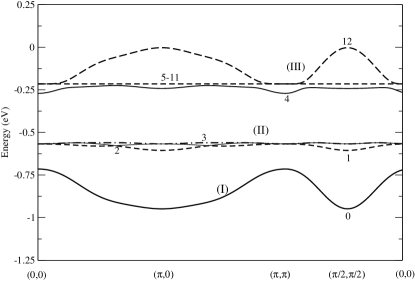
Figure 11: The higher energy string excitations obtained by diagonalizing the $t-J$ Hamiltonian in the subspace spanned by the 161 states illustrated in Fig. 9 using $J/t=0.3$ and $t=0.4eV$. The lowest energy state is labeled 0 and it is the same as the dispersion presented in Fig. 10. The lowest lying excited states are three nearly degenerate excited states labeled 1,2,3 (which form the group labeled (II)). Following a gap there is a group of states labeled (III) which includes the fourth state and the next six states, namely, 5-11 which are degenerate. In addition, it includes the 12th excited state which follows a mirror-like dispersion to the ground state.

In Fig. 11 we give the energy of the string excitations found by diagonalizing the $t-J$ Hamiltonian in the subspace of the string states shown in Fig. 9 along the same Brillouin zone path, namely, from $(0,0)\to(\pi,0)\to(\pi,\pi)\to(0,0)$. These states form bands and we can identify what we have labeled as II and III in the previous discussion of Sec. II and Sec. III. Namely, the three nearly degenerate excited states labeled as 1,2 and 3 form the band II and the nine states labeled 4-12 form the group labeled III in our previous discussion of Sec. II. Notice that their energy is the same to those of the peaks labeled II and III in Fig. 1 and Fig. 4. In addition, their dispersion is very similar, namely, II is almost dispersionless and III along the $(0,0)$ to $(\pi/2,\pi/2)$ cut (Fig. 1) moves closer to the peaks I and II near $(0,0)$ and further away from the peaks I and II near $(\pi/2,\pi/2)$.

Therefore, the conclusion of this study is that the short-range string correlations are very important in determining the energetics of the hole dynamics. One expects that long wavelength spin fluctuations to be important in the ordered quantum antiferromagnet. However, when the antiferromagnetic order is destroyed as the doping level is increased, while the long wavelength spin-fluctuation excitations are not well-defined, the string excitations still remain and they can quantitatively account for the short wavelength dynamics. With these findings in mind we proceed to show that these string correlations give rise to a pairing mechanism which is characterized by a relatively strong pairing interaction, namely, significantly stronger that the effective interaction due to exchange of antiferromagnetic spin-fluctuations.

IV.2 String-mediated pairing

In this paper, inspired by the findings of the photoemission measurements and our suggestion that they provide evidence for the existence of string excitations even at optimal doping, we suggest that the pairing mechanism found numerically in the $t-J$ modelBM ; KM is mediated by strings.

The rather simple calculation of the previous subsection suggests that states of unbroken strings are the main contributors to the single-hole dispersion. In Fig. 12 a pair of holes A and B is shown connected by a string of overturned spins in an otherwise idealized Néel ordered background with no spin deviation. First, in order to facilitate the discussion let us consider states with unbroken strings connecting the two holes. The two holes experience a potential linearly rising as a function of the length of the string between them. Namely, when either hole is moved in such a way that the distance between the holes is increased as shown in Fig. 12(b), it stretches the length of the string of overturned spins and the potential energy increases. On the other hand, each hole feels a down-hill potential toward each other because by moving along the path, defined by their mutually connecting string, they repair the overturned spins as indicated in Fig. 12(c).

In addition, it can be demonstrated using Fig. 12 (a,b,d) that when there are such string correlations between two holes, the entire string bipolaron can move through the lattice with an effective mass which is lighter than that of a single hole. In leading order the hole has to make two successive hops followed by a pair spin-flip in order for the hole to move through the lattice. This is of higher order than the process illustrated in Fig. 12(a,b,d) where first the hole A hops (transition from (a) to (b)) momentarily lengthening the string and this is followed by a hop of the second hole B (transition from (b) to (d)) which takes the down-hill path formed by the string. Notice that the configuration (d) has the same length of the string as the starting configuration A, but the hole string bipolaron has moved and, thus, gains delocalization energy.

Figure 12: (a) A pair of holes (A) and (B) marked by o’s are connected by a string of overturn spins. (b) For either hole to attempt to unbind itself from the other leads to lengthening the string which is energetically costly. (c) For either hole to attempt to hop closer to the other hole it is energetically favorable. (d) The string configuration of pair of holes (a) can be momentarily lengthened by allowing hole B to hop as shown in (b) and finally the length of the string is restored to original length size by allowing hole A to hop along the string as in configuration (d).

A variational wave function to describe such a pair of holes of zero net momentum may be written as follows:

$$|\psi_{2}\rangle = \sum_{{\bf r}_{1},{\bf r}_{2}}e^{-i{\bf k}\cdot({\bf r}_{1}-{\bf r}_{2})}g({\bf r}_{2}-{\bf r}_{1})$$ (7)

$$\times \Bigl{[}1+\sum_{{\bf s}({\bf r}_{1},{\bf r}_{2})}\Phi(Y({\bf r}_{1},{\bf r}_{2}))\hat{Y}({\bf r}_{1},{\bf r}_{2})\Bigr{]}\hat{T}_{{\bf r}_{1}}\hat{T}_{{\bf r}_{2}}|0\rangle,$$

where $Y({\bf r}_{1},{\bf r}_{2})$ is a connected path connecting the sites ${\bf r}_{1}$ and ${\bf r}_{2}$ which are the location of the holes and $\Phi(Y({\bf r}_{1},{\bf r}_{2})))$ is a function of the path which defines the string and it is expected to be a decreasing function of the length of the path. The state $|0\rangle$ is the no-hole state given by Eq. 6 and the operators $T_{{\bf r}_{1,2}}$ are given by Eq. 4 and they create the strings attached to each hole. The operator $\hat{Y}({\bf r}_{1},{\bf r}_{2})$ is a product of hole-hop operators $\hat{P}_{ij}$ (defined after Eq. 5) along the path connecting the two holes defined by $Y({\bf r}_{1},{\bf r}_{2})$. When this operator acts on the Néel state creates states, such as the state illustrated in Fig. 12(a), where the holes located at ${\bf r}_{1}$ and ${\bf r}_{2}$ are connected with a string of overturned spins in an otherwise perfectly ordered Néel spin lattice. The function $g({\bf r}_{2}-{\bf r}_{1})$ gives the symmetry of the two hole state and for $d_{x^{2}-y^{2}}$ symmetry it changes only its sign (keeping the same magnitude) for a $\pi/2$ rotation.

A similar variational state built upon such a basis of string states which included the effect of background spin fluctuations was studied in Ref. BM, and it was also used as the initial state for the Green’s function Monte Carlo calculation. It was found that two holes bind in a state with the $d_{x^{2}-y^{2}}$ symmetry for $J/t$ greater than about $0.27$.

Let us restrict ourselves in the subspace where the two holes are connected by an unbroken string. This implies that the spin-fluctuation part of the $t-J$ model gives zero contribution to matrix elements in this subspace. In order to illustrate that, let us consider a two-hole state with an unbroken string mediated between the two holes such as any state from Fig. 12. When applying the pair spin-flip operator of the $t-J$ model on such a state, it will always produce a state with a broken string and, thus, it takes us outside the Hilbert space of states with all-connected strings. As a consequence the result of the calculation of the binding energy $\Delta$ of two holes in this restricted subspace, is very similar to that using the $t-J_{z}$ model with $J_{z}=J$. Using a diagrammatic approach Chernyshev and Leungchernyshev found that there is strong binding in $p$ and $d$ wave symmetry between two holes in the $t-J_{z}$ model. In addition, calculation of the quantity $\Delta$ has been carried out for the $t-J_{z}$ model using exact diagonalizationriera on lattices with up to 50 sites and it was found that the two holes bind in a $d_{x^{2}-y^{2}}$ for $J/t$ greater than $\sim 0.2$.

We would like to go back and discuss the fact that the spin fluctuation operator can break the string connecting the two holes. These processes, however, compete with processes which lower the pair hole energy discussed previously by allowing the pair to delocalize when the connecting string is present and with other processes which accommodate the hole motion of each hole within the string. Namely, when one hole creates a string, another hole near the first hole, has increased probability to follow the string created by the first hole, thus, they are experiencing pairing correlations. Therefore, on variational grounds we believe that the pairs of holes, depending on the parameter regime, may have string-mediated pairing correlations.

Here, we would like to discuss what happens when the level of doping increases. As it has been discussed earlier in this paper, in order for the string-like correlations to be effective, we do not need to require long range antiferromagnetic(AF) order. This is because the cuprates are described by an intermediate parameter regime, where $t/J\sim 3$. In this intermediate regime, we found that strings of length only three lattice spacings can reproduce the single hole dispersion reasonably well (see Fig. 10). Therefore, short-range string correlations only require that AF spin-spin correlations exist up to such rather short distance of two or three lattice spacings away from the hole. This requirement is believed to be true even at optimal doping. Hence, we believe that such short-range AF spin correlations, required for the string mediated interaction between pairs of holes, could still be present in the cuprates even at optimum doping.

V conclusions

Our findings suggest a new framework to understand doped quantum antiferromagnets and possibly the pairing mechanism in the cuprate superconductors.

First, we illustrated that the high resolution ARPES studiesronning ; graf from cuprates suggest the following.

(a) The hole in the doped quantum antiferromagnet becomes a rather well-defined quasiparticle and it is always attached to a string of overturned spins which follows the hole in its motion via processes of coherent pair spin-flip which lead to a reassignment of the hole birth site.

(b) The high energy features and dispersion discussed in this paper, which are seen in ARPES, can be understood as “internal” excitations of the “spin-polaron”. In this paper, it is shown that these excitations are responsible for the vanishing of the quasiparticle from the lowest string state at the $\Gamma$ point and for the transfer of spectral weight to higher energy string excitations. In addition, they may be responsible for the high energy anomalous dispersion found in the most recent ARPES studiesronning ; graf .

Second, a simple model is postulated where only states of holes connected with unbroken strings of overturned spins are retained. This model gives a very good quantitative account of both the quasiparticle dispersion and the higher energy string excitations.

Third, motivated by both the fact that our simple model of string excitations can explain the results of the $t-J$ model and the fact that the new features of ARPES studies can be interpreted as arising from such string excitations, we further consider the role of such string excitations in the pairing mechanism. We show that pairs of holes experience attractive pairing interaction due to exchange of such string excitations. Namely, when one of the holes creates such a string of overturned spins in order to be able to move, another hole takes advantage of the created path of overturned spins and follows it, thus, restoring part of the destroyed antiferromagnetic order.

The proposed pairing mechanism could be superior to those of models which are based on exchange of antiferromagnetic spin fluctuations for the following two main reasons: (i) As we discussed in the previous section, our model does not require long range antiferromagnetic order but rather short-range antiferromagnetic spin correlations. (ii) The pairing energy scale is much larger than the typical energy scale that a spin-fluctuation exchange model would give, since the effective attraction in our string-exchange model arises from exchange of short-range high energy excitations.

VI Acknowledgments

I would like to thank P. Coleman and V. Dobrosavljevic for discussions. This work was supported by NASA under grant No NAG-2867.

References

- (1) B. O. Wells et al., Phys. Rev. Lett. 74, 964 (1995).
- (2) A. Damascelli, Z. Hussain, Z. -X. Shen, Rev. Mod. Phys. 75, 473 (2003). See references therein.
- (3) F. Ronning, et al., Phys. Rev. B 71, 094518 (2005).
- (4) J. Graf, el al., cond-mat/0607319.
- (5) Z. Liu and E. Manousakis, Phys. Rev. B 44, 2414 (1991). and , 45, 2425 (1992).
- (6) E. Dagotto, Rev. Mod. Phys., 66, 763 (1994) and references therein.
- (7) E. Manousakis, Rev. Mod. Phys. 63, 1 (1991).
- (8) E. Manousakis, in Electronic, optoelectronic and magnetic thin films, ed. J. M. Marshall, N. Kirov and A. Vavrek, pg 168, J. Wiley and Sons, (New York, 1995).
- (9) A. Nazarenko et al., Phys. Rev. B 51, 8676 (1995).
- (10) B. Kyung and R. A. Ferrell, Phys. Rev. B 54, 10125 (1996).
- (11) T. K. Lee and C. T. Shih, Phys. Rev. B 55, 5983 (1997).
- (12) T. Xiang and J. M. Wheatley, Phys. Rev. B 54, R12653 (1996).
- (13) V. I. Belinicher, et al., Phys. Rev. B 54, 14914 (1996).
- (14) R. Eder, et al., Phys. Rev. B 55, R3414 (1997).
- (15) C. Kim et al., Phys. Rev. Lett. 80, 4245 (1998).
- (16) B. Shraiman and E. Siggia, Phys. Rev. Lett. 60, 740 (1988);
- (17) B. Shraiman and E. Siggia, Phys. Rev. Lett. 61, 467 (1988);
- (18) B. Shraiman and E. Siggia, Phys. Rev. Lett. 62,1564 (1989);
- (19) S. Trugman, Phys. Rev. B 37, 1597 (1988).
- (20) T. Barnes, et al., Phys. Rev. B 40, 10977 (1989).
- (21) E. Dagotto, et al., Phys. Rev. B 41, 9049 (1990).
- (22) V. Elser, D. Huse, B. Shraiman, and E. Siggia, Phys. Rev. B 41, 6715 (1990).
- (23) C. Kane, P. Lee, and N. Read, Phys. Rev. B 39, 6880 (1989).
- (24) F. Marsiglio, A. Ruckenstein, S. Schmitt-Rink and C. Varma, Phys. Rev. B 43, 10 882 (1991).
- (25) G. Martínez and P. Horsch, Phys. Rev. B 44, 317(1991).
- (26) P. Srivastava and A. Singh, Phys. Rev. B 70, 115103 (2004).
- (27) E. Manousakis, Phys. Lett. A 362, 86 (2007).
- (28) A. S. Mishchenko, N. Nagaosa, Phys. Rev. Lett., 93, 036402 (2004).
- (29) F. C. Zhang and T. M. Rice, Phys. Rev .B 37, 3759 (1988).
- (30) M. Boninsegni and E. Manousakis, Phys. Rev. B 45, 4877 (1992). , Phys. Rev. B 46, 560 (1992).
- (31) Z. Liu and E. Manousakis, Phys. Rev. B 44, 2414 (1991).
- (32) M. Boninsegni and E. Manousakis, Phys. Rev. B 46, 560-563 (1992).
- (33) M. Boninsegni and E. Manousakis, Phys. Rev. B 47, 11897 (1993).
- (34) E. Kaxiras and E. Manousakis, Phys. Rev. B 38, 866-869 (1988).
- (35) J. Riera and E. Dagotto, Phys. Rev. B 47, 15346 (1993).
- (36) A. L. Chernyshev, P. W. Leung, Phys. Rev. B 60, 1592 (1999).