On the stress and torque tensors in fluid membranes

Abstract. – We derive the membrane elastic stress and torque tensors using the standard Helfrich model and a direct variational method in which the edges of a membrane are infinitesimally translated and rotated. We give simple expressions of the stress and torque tensors both in the local tangent frame and in projection onto a fixed frame. We recover and extend the results of Capovilla and Guven [J. Phys. A, 2002, 35, 6233], which were obtained using covariant geometry and Noether’s theorem: we show that the Gaussian rigidity contributes to the torque tensor and we include the effect of a surface potential in the stress tensor. Many interesting situations may be investigated directly using force and torque balances instead of full energy minimization. As examples, we consider the force exerted at the end of a membrane tubule, membrane adhesion and domain contact conditions.

1 Introduction

Lipid molecules dissolved in water spontaneously form bilayer membranes, which may be idealized as fluid, incompressible surfaces with superficial tension and bending rigidity [1]. These membranes, which form vesicles or lamellar phases, are widely studied in complex fluid physics and in biology, as model systems of cell walls or encapsulation agents, e.g., in the medical and cosmetic industry [2].

The elasticity associated with the deformations and fluctuations of fluid membranes is given by a surface integral known as the Helfrich Hamiltonian [3],

$$F=\int\!dA\left[\sigma+\frac{\kappa}{2}\left(c_{1}+c_{2}-c_{0}\right)^{2}+\bar{\kappa}\,c_{1}c_{2}\right].$$ (1)

The constant $\sigma$, usually called the “surface tension”, is better understood as a chemical potential per surface unit fixing the value of the (average) membrane area. Indeed, membranes have a fixed number of lipids, hence essentially a fixed total area $A$. Instead of fixing $A$, it is usually more convenient to let $A$ vary freely while adding a term $\sigma A$ to the Hamiltonian in the canonical probability distribution (very much like one adds a term $-\mu\,N$ in order to fix the average value of $N$ in the grand-canonical ensemble). The last two terms correspond to the most general quadratic curvature energy for an isotropic surface. The parameters $c_{1}$ and $c_{2}$ are the two principal curvatures, defined locally at each point of the surface along two orthogonal directions. The term with coefficient $\kappa$ (bending rigidity) favors a global curvature $c_{1}+c_{2}$ equal to some constant $c_{0}$ characteristic of the membrane. If the two monolayers forming the membrane are identical, $c_{0}=0$ by symmetry, and the bending term simply favors flatness. The term with coefficient $\bar{\kappa}$ (Gaussian rigidity constant) either favors spherical-like curvature, i.e., $c_{1}c_{2}>0$, if $\bar{\kappa}<0$, or saddle-like curvature, i.e., $c_{1}c_{2}<0$, if $\bar{\kappa}>0$. Note that it is often omitted, since the integral $\int dA\,c_{1}c_{2}$ on a closed surface only depends on the topology of the surface (Gauss-Bonnet theorem).

Using covariant differential geometry and Noether’s theorem, Capovilla and Guven [4] have recently derived the stress and torque tensors associated with the Helfrich Hamiltonian. In this paper, we revisit these two quantities. Although we use the so-called Monge gauge for small deformations with respect to a flat membrane, our results in the local tangent frame bear no difference with the general covariant expression of [4]. This is actually not surprising, since the Helfrich Hamiltonian is quadratic in the local curvature. We derive the stress and torque tensors using a direct and simple method based on examining the elastic work done when translating or rotating infinitesimally the edges of a membrane. We thus obtain the “projected” stress and torque tensors, all quantities referring to a basal plane above which the membrane stands. We may then easily express all quantities in the local tangent frame, thus obtaining very simple expressions. Apart from the differences in the formulation, there are three new results with respect to Ref. [4]: i) the Gaussian rigidity ($\bar{\kappa}$) is shown to contribute to the torque tensor, ii) the contribution of an external potential $V$ arising from a substrate is discussed and included in the stress tensor, iii) the stress and torque tensors are given both as “local” and “projected” quantities, the latter formulation being useful when one needs to integrate the force exerted by the membrane through an extended contour.

2 Derivation of the stress and torque tensors

The stress tensor, $\bm{\Sigma}$, relating linearly the force exerted by the membrane through an infinitesimal cut to the vector normal to the cut and proportional to its length is a tensor with $3\times 2=6$ components [4]. Indeed, the force is a three-dimensional vector (usually not tangent to the surface), while the vector normal to the cut may be taken as lying within the surface and thus needs only be described by a two-dimensional vector. The same holds for the torque tensor $\mathbf{T}$ which provides the elementary torque exchanged through a cut.

Let us consider a membrane parametrized by its height $z=h(x,y)$ above a reference plane $(x,y)$ in an orthonormal basis $(x,y,z)$. Assuming that the membrane is only weakly deformed with respect to the plane $(x,y)$, we shall neglect everywhere terms of order higher than 2 in the derivatives of $h$. Our aim, first, is to calculate the “projected” stress tensor $\bm{\Sigma}=\Sigma_{ij}\mathbf{e}_{i}\otimes\mathbf{e}_{j}+\Sigma_{zj}\mathbf{e}_{z}\otimes\mathbf{e}_{j}$ and the “projected” torque tensor (per unit length) $\mathbf{T}=T_{ij}\mathbf{e}_{i}\otimes\mathbf{e}_{j}+T_{zj}\mathbf{e}_{z}\otimes\mathbf{e}_{j}$ in the fixed frame $(x,y,z)$. Here and in the following, Latin indices stand only for $x$ or for $y$. These tensors are defined as follows. Consider first an infinitesimal cut of length $d\ell^{\prime}$ in the membrane, separating two regions (see Fig. 1). Consider, next, the projection of this infinitesimal cut onto $(x,y)$, of length $d\ell$ and normal $\mathbf{m}$ pointing towards the inside of region n${}^{\circ}1$. By virtue of linearity, the infinitesimal force $d\bm{\phi}_{1\to 2}$ and the infinitesimal torque $d\bm{\tau}_{1\to 2}$ that region n${}^{\circ}1$ exerts onto region n${}^{\circ}2$ through the cut $\mathbf{m}\,d\ell$ (for a given membrane configuration) are given by

$$d\bm{\phi}_{\mathrm{1\to 2}}\!\! = \!\!\mathbf{\Sigma}\cdot\mathbf{m}\,d\ell\,\,=\,\,\mathbf{e}_{i}\,\Sigma_{ij}m_{j}d\ell+\mathbf{e}_{z}\,\Sigma_{zj}m_{j}d\ell\,,\quad$$ (2)

$$d\bm{\tau}_{\mathrm{1\to 2}}\!\! = \!\!\mathbf{T}\cdot\mathbf{m}\,d\ell\,\,=\,\,\mathbf{e}_{i}\,T_{ij}m_{j}d\ell+\,\mathbf{e}_{z}\,T_{zj}m_{j}d\ell\,.$$ (3)

Summation over repeated indices will be implicit throughout. Note that with the above sign convention, $\bm{\Sigma}$ can be considered as a (tensorial) mechanical tension.

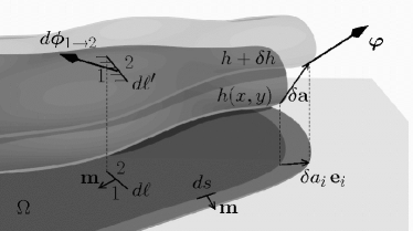
Figure 1: Configuration and notations used in the derivation of the “projected” stress and torque tensors. The membrane $h(x,y)$ standing above domain $\Omega$ (dark grey) is deformed and its edges are translated by $\delta\mathbf{a}$. The deformed membrane, $h(x,y)+\delta h(x,y)$, is drawn in transparency and its projection onto the basal plane is drawn in a lighter grey. The force density $\bm{\varphi}$ acting along the border and the force $d\bm{\phi}_{1\to 2}$ exchanged through the cut $d\ell^{\prime}$ are shown (for the sake of clarity, the torques are not shown). In the “projected” formulation, the stress and torque tensors are defined with respect to the projected cut $\mathbf{m}\,d\ell$ lying on the basal plane instead of the actual cut $d\ell^{\prime}$ lying within the membrane.

2.1 General derivation

Consider now a deformed membrane (weakly departing from a plane) which is at equilibrium under the action of external forces $\bm{\varphi}$ and external torques $\bm{\tau}$ acting along its edges (Fig. 1). Let $\Omega$ be the domain of $(x,y)$ above which the membrane $h(x,y)$ is defined and $\partial\Omega$ its border, of curvilinear abscissa $s$ and outer normal $\mathbf{m}$. The membrane elastic free-energy has the general form:

$$F=\int_{\Omega}\!dx\,dy\,f(\{\partial_{i}h\},\{\partial_{i}\partial_{k}h\})\,.$$ (4)

Calling $\mathbf{r}=(x,y)$, we vary the membrane shape: $h(\mathbf{r})\to h^{\prime}(\mathbf{r})=h(\mathbf{r})+\delta h(\mathbf{r})$, arbitrarily, while translating the membrane edges by $\delta\mathbf{a}(\mathbf{r})=\delta a_{i}(\mathbf{r})\,\mathbf{e}_{i}+\delta a_{z}(\mathbf{r})\,\mathbf{e}_{z}$ (recall that Latin indices stand only for $x$ or $y$). We also apply to the borderline normal $\mathbf{n}$ an infinitesimal rotation $\delta\bm{\omega}(\mathbf{r})=\delta\omega_{i}(\mathbf{r})\,\mathbf{e}_{i}+\delta\omega_{z}(\mathbf{r})\,\mathbf{e}_{z}$. Integrating twice by parts, the free-energy variation may be cast into the form :

$$\delta F\!\! = \!\!\int_{\Omega}\!dx\,dy\,\frac{\delta{F}}{\delta h}\delta h+\int_{\partial\Omega}\!ds\,m_{i}\Bigg{[}f\,\delta a_{i}+\frac{\partial f}{\partial(\partial_{i}h)}\delta h$$ (5)

$$+\frac{\partial f}{\partial(\partial_{i}\partial_{k}h)}\partial_{k}\delta h-\partial_{k}\!\left(\frac{\partial f}{\partial(\partial_{i}\partial_{k}h)}\right)\delta h\Bigg{]}\,.$$

The border translation and rotation conditions imply $\forall\mathbf{r}\in{\partial\Omega}$, $h^{\prime}(\mathbf{r}+\delta a_{i}(\mathbf{r})\,\mathbf{e}_{i})=h(\mathbf{r})+\delta a_{z}(\mathbf{r})$ and $\partial_{k}h^{\prime}(\mathbf{r}+\delta a_{i}(\mathbf{r})\,\mathbf{e}_{i})=\partial_{k}h(\mathbf{r})-\epsilon_{k\ell}\,\delta\omega_{\ell}(\mathbf{r})-\delta\omega_{z}(\mathbf{r})\,\epsilon_{k\ell}\,\partial_{\ell}h(\mathbf{r})$, where $\epsilon_{k\ell}$ is the Levi-Civita antisymmetric symbol. The latter relation follows from $\delta\mathbf{n}=\delta\bm{\omega}\times\mathbf{n}$ and $\mathbf{n}\simeq\mathbf{e}_{z}-(\partial_{i}h)\mathbf{e}_{i}$. Hence, to first order in $\delta h$, we obtain the consistency relations at the border :

$$\delta h\!\! = \!\!\delta a_{z}-\delta a_{j}\,\partial_{j}h$$ (6)

$$\partial_{k}\delta h\!\! =\!\! -\epsilon_{k\ell}\,\delta\omega_{\ell}-\delta\omega_{z}\,\epsilon_{k\ell}\,\partial_{\ell}h-\delta a_{j}\,\partial_{j}\partial_{k}h\,.$$ (7)

At equilibrium, the free-energy variation $\delta F$ must be equal to the external work $\delta W$, which implies

$$0=\delta F-\delta W=\delta F-\int_{\partial\Omega}\,ds\,(\bm{\varphi}\cdot\delta\mathbf{a}+\bm{\tau}\cdot\delta\bm{\omega})\,.$$ (8)

Using Eqs. (5)–(8) and identifying the terms in factor of $\delta a_{j}$, $\delta a_{z}$, $\delta\omega_{\ell}$ et $\delta\omega_{z}$, which must vanish everywhere because of the arbitrariness of the shape variation, we obtain $\varphi_{j}=m_{i}\,\Sigma_{ji}$, $\varphi_{z}=m_{i}\,\Sigma_{zi}$, $\tau_{\ell}=m_{i}\,T_{\ell i}$ et $\tau_{z}=m_{i}\,T_{zi}$, yielding

$$\Sigma_{ij} = f\,\delta_{ij}-\frac{\partial f}{\partial(\partial_{j}h)}\,\partial_{i}h-\frac{\partial f}{\partial(\partial_{j}\partial_{k}h)}\,\partial_{i}\partial_{k}h$$ (9)

$$+ \partial_{k}\!\left(\frac{\partial f}{\partial(\partial_{j}\partial_{k}h)}\right)\partial_{i}h\,,$$

$$\Sigma_{zj} = \frac{\partial f}{\partial(\partial_{j}h)}-\partial_{k}\frac{\partial f}{\partial(\partial_{j}\partial_{k}h)}\,,$$ (10)

$$T_{ij} = \epsilon_{ik}\,\frac{\partial f}{\partial(\partial_{j}\partial_{k}h)}\,,$$ (11)

$$T_{zj} = -\epsilon_{k\ell}\,\frac{\partial f}{\partial(\partial_{j}\partial_{k}h)}\,\partial_{\ell}h\,,$$ (12)

which constitute the formal expressions of the “projected” stress and torque tensors.

2.1.1 Stress tensor divergence

Directly differentiating the components of the stress tensor yields $\partial_{j}\Sigma_{zj}=-\delta F/\delta h$ and $\partial_{j}\Sigma_{ij}=(\partial_{i}h)\,\delta F/\delta h$, where $\delta F/\delta h=-\partial_{i}[\partial f/\partial(\partial_{i}h)]+\partial_{i}\partial_{j}[\partial f/\partial(\partial_{i}\partial_{j}h)]$ is the standard Euler-Lagrange term. We recognize in fact the equation $\bm{\nabla}\cdot\bm{\Sigma}=-(\delta F/\delta h)\,\mathbf{n}$, since at lowest order, the membrane normal is given by $\mathbf{n}\simeq\mathbf{e}_{z}-(\partial_{i}h)\mathbf{e}_{i}$. This equation correctly states that the restoring elastic force density exerted by the membrane is $-(\delta F/\delta h)\,\mathbf{n}$. This is indeed a well-known starting point in dynamical descriptions. At equilibrium, since $\delta F/\delta h=0$, we obtain

$$\partial_{j}\Sigma_{zj}=\partial_{j}\Sigma_{ij}=0\,,$$ (13)

i.e., the stress tensor is divergence-free.

2.2 Case of the Helfrich Hamiltonian

In the particular case of the Helfrich Hamiltonian (1), we obtain to second order in the derivatives of $h$, the following elastic energy density:

$$f=\sigma+\frac{\sigma}{2}\left(\nabla h\right)^{2}+\frac{\kappa}{2}\left(\nabla^{2}h-c_{0}\right)^{2}+\bar{f}\,,$$ (14)

where $\bar{f}=\bar{\kappa}\,\rm{det}(\partial_{i}\partial_{j}h)=\frac{1}{2}\bar{\kappa}\,[(\nabla^{2}h)^{2}-(\partial_{i}\partial_{j}h)(\partial_{i}\partial_{j}h)]$ is the Gaussian curvature contribution. This yields $\partial f/\partial(\partial_{j}h)=\sigma\,\partial_{j}h$ and $\partial f/\partial(\partial_{j}\partial_{k}h)=(\kappa+\bar{\kappa})\,\delta_{jk}\nabla^{2}h-\bar{\kappa}\,\partial_{j}\partial_{k}h-\kappa\,c_{0}\,\delta_{jk}$. Since $(\partial_{i}\partial_{k}h)\times\partial\bar{f}/\partial(\partial_{j}\partial_{k}h)=-\bar{f}\delta_{ij}$ and $\partial_{k}[\partial\bar{f}/\partial(\partial_{j}\partial_{k}h)]=0$, we obtain explicitely

$$\Sigma_{ij} = (f-\bar{f})\,\delta_{ij}-\sigma\left(\partial_{i}h\right)\left(\partial_{j}h\right)$$ (15)

$$- \kappa\left(\nabla^{2}h-c_{0}\right)\partial_{i}\partial_{j}h+\kappa\left(\partial_{i}h\right)\,\partial_{j}\nabla^{2}h\,,$$

$$\Sigma_{zj} = \sigma\,\partial_{j}h-\kappa\,\partial_{j}\nabla^{2}h\,,$$ (16)

$$T_{ij} = \left(\kappa+\bar{\kappa}\right)\nabla^{2}h\,\epsilon_{ij}-\bar{\kappa}\,\epsilon_{ik}\,\partial_{j}\partial_{k}h-\kappa\,c_{0}\,\epsilon_{ij}\,,\quad$$ (17)

$$T_{zj} = -\left(\kappa+\bar{\kappa}\right)\left(\nabla^{2}h\right)\epsilon_{j\ell}\,\partial_{\ell}h$$ (18)

$$+ \bar{\kappa}\,\epsilon_{k\ell}\left(\partial_{j}\partial_{k}h\right)\,\partial_{\ell}h+\kappa\,c_{0}\,\epsilon_{j\ell}\,\partial_{\ell}h\,.$$

Note that the contributions involving $\bar{\kappa}$ cancel altogether in the expression of $\bm{\Sigma}$, but not in the expressions of $\mathbf{T}$.

These four equations are our central result. Recall that they are valid only up to second order in the derivatives of $h$. Recall also that they give the components of the “projected” stress and torque tensors : not only the components are projected along the fixed basis $(x,y,z)$, but also the elementary cut $m_{j}\,d\ell$ by which they must be multiplied is, by definition, the projection onto the reference plane of a cut within the membrane surface.

More explicitly, the Cartesian components of the “projected” stress and torque tensors (in the case $c_{0}=0$ for the sake of simplicity) are given by

$$\Sigma_{xx} = \sigma+\frac{\sigma}{2}\left[\left(\partial_{y}h\right)^{2}-\left(\partial_{x}h\right)^{2}\right]$$ (19)

$$+ \frac{\kappa}{2}\left[\left(\partial^{2}_{y}h\right)^{2}-\left(\partial^{2}_{x}h\right)^{2}\right]+\kappa\left(\partial_{x}h\right)\partial_{x}\nabla^{2}h\,,\quad$$

$$\Sigma_{xy} = -\sigma\left(\partial_{x}h\right)\left(\partial_{y}h\right)-\kappa\left(\partial_{x}\partial_{y}h\right)\nabla^{2}h$$ (20)

$$+ \kappa\left(\partial_{x}h\right)\partial_{y}\nabla^{2}h\,,$$

$$\Sigma_{zx} = \sigma\,\partial_{x}h-\kappa\,\partial_{x}\nabla^{2}h\,.$$ (21)

The other components follow by exchanging $x$ and $y$. For the torque tensor, we obtain explicitly

$$T_{xx} = -\bar{\kappa}\,\partial_{x}\partial_{y}h\,,$$ (22)

$$T_{xy} = \kappa\,\nabla^{2}h+\bar{\kappa}\,\partial^{2}_{x}h\,$$ (23)

$$T_{yx} = -\kappa\,\nabla^{2}h-\bar{\kappa}\,\partial^{2}_{y}h\,$$ (24)

$$T_{yy} = \bar{\kappa}\,\partial_{x}\partial_{y}h\,,$$ (25)

$$T_{zx} = -\kappa\left(\nabla^{2}h\right)\partial_{y}h$$ (26)

$$- \bar{\kappa}\left(\partial_{y}^{2}h\right)\partial_{y}h-\bar{\kappa}\left(\partial_{x}\partial_{y}h\right)\partial_{x}h\,$$

$$T_{zy} = \kappa\left(\nabla^{2}h\right)\partial_{x}h$$ (27)

$$+ \bar{\kappa}\left(\partial_{x}^{2}h\right)\partial_{x}h+\bar{\kappa}\left(\partial_{x}\partial_{y}h\right)\partial_{y}h\,.$$

2.3 Expressions in the tangent, principal frame

Locally, for a membrane with a given fixed shape, it is always possible to choose the frame $(x,y,z)=(X,Y,Z)$ in such a way that it is tangent to the membrane and has $X$ and $Y$ oriented along the directions of principal curvatures. For the sake of simplicity, we shall first consider the case $c_{0}=0$. Hence, in the tangent, principal frame, we have $\partial_{X}h=\partial_{Y}h=\partial_{X}\partial_{Y}h=0$, and $\partial^{2}_{X}h=C_{X}$ and $\partial^{2}_{Y}h=C_{Y}$, where $C_{X}$ and $C_{Y}$ are the principal curvatures.

For the stress tensor, either from Eqs. (15)–(16), or Eqs. (19)–(21), this yields

$$\Sigma_{XX} = \sigma+\frac{\kappa}{2}C_{Y}^{2}-\frac{\kappa}{2}C_{X}^{2}\,,$$ (28)

$$\Sigma_{YX} = 0\,,$$ (29)

$$\Sigma_{ZX} = -\kappa\,\partial_{X}C\,,$$ (30)

where $\partial_{X}C$ is the gradient along $X$ of the sum $C$ of the principal curvatures. These expressions agree with the general covariant formula of Ref. [4] (see also Ref. [5]). The components $\Sigma_{YY}$, $\Sigma_{XY}$, $\Sigma_{ZY}$ simply follow by exchanging $X$ and $Y$ in the above expressions. Hence, in the tangential frame, the force exerted by the membrane through a cut parallel to a direction of principal curvature has a tangential component perpendicular to the cut and also a component normal to the membrane (see Fig. 2a). In the case $c_{0}\neq 0$, the contribution $\Sigma_{XX}^{(0)}=\frac{1}{2}\kappa\,c_{0}^{2}-\kappa\,c_{0}\,C_{Y}$ must be added to $\Sigma_{XX}$.

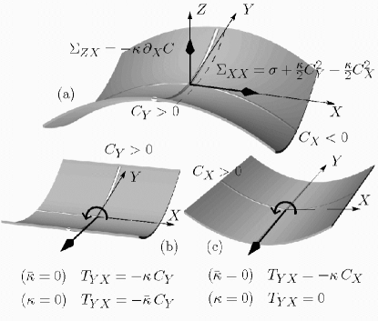
Figure 2: (a) Components of the stress tensor in the tangent, principal frame (the axes $X$ and $Y$ are oriented along the principal curvatures directions), for $c_{0}=0$. The quantity $\Sigma_{XX}$ is the force per unit length exerted along $X$ by the region $X>0$ onto the region $X<0$ through a cut normal to to the $X$ axis (i.e., parallel to the $Y$ axis). Likewise, $\Sigma_{ZX}$ represent the component along $Z$ of the same force. (b)–(c) In the tangent, principal frame, the torque exchanged through a cut parallel to a principal direction is tangent to the membrane and parallel to the cut. Several situations are depicted, showing the contributions from $\kappa$ and $\bar{\kappa}$ (for $\bar{\kappa}>0$ and $c_{0}=0$).

For the torque tensor, we get

$$T_{XX} = 0\,,$$ (31)

$$T_{YX} = -\kappa\left(C_{X}+C_{Y}\right)-\bar{\kappa}\,C_{Y}\,,$$ (32)

$$T_{ZX} = 0\,.$$ (33)

The components $T_{YY}$, $T_{XY}$ and $T_{ZY}$ are obtained by exchanging $X$ and $Y$ and multiplying by $-1$ (due to the presence of the Levi-Civita antisymmetric symbol). In the case $c_{0}\neq 0$, the contribution $T_{YX}^{(0)}=\kappa\,c_{0}$ must be added to $T_{YX}$.

The formula $\Sigma_{XX}=\sigma+\frac{1}{2}\kappa\,C_{Y}^{2}-\frac{1}{2}\kappa\,C_{X}^{2}$ may be interpreted as follows. It is given by the sum of the first and the third terms of Eq. (9) (the other two terms vanishing in the tangential frame). The first term, disregarding the Gaussian contribution, is $f\delta_{ij}=\sigma+\frac{\kappa}{2}(C_{X}+C_{Y})^{2}$; the third term is $-(\partial_{i}\partial_{k}h)\,\partial f/\partial(\partial_{j}\partial_{k}h)=-\kappa(C_{X}+C_{Y})C_{X}$. Indeed, if the membrane is retracted in the direction perpendicular to the cut (dashed line in Fig. 2a), there is both an energy gain associated with removing a band of membrane having an energy density $f$ (first term), and, since this operation must be done at constant orientation of the membrane normal to prevent torques work, a change in curvature energy if $C_{X}$ is non-zero (third term).

To check the validity of the formulas for the torque tensor, consider first the case $\bar{\kappa}=0$ and $\kappa\neq 0$, where $T_{YX}=-\kappa(C_{X}+C_{Y})$. As can be seen in Fig. 2, the effect of $T_{YX}$ (i.e., the tendency of the region $X>0$) is to curve the cylinder into a saddle in Fig. 2b or to reduce the cylindrical curvature in Fig. 2c : in both cases there is a gain in bending energy since the mean curvature is lowered. Next, consider the case $\bar{\kappa}>0$ and $\kappa=0$, where $T_{YX}=-\bar{\kappa}\,C_{Y}$. The tendency of the region $X>0$ is to curve the cylinder into a favorable saddle $(\bar{\kappa}>0)$ in Fig. 2b, while there is no torque in Fig. 2c because the Gaussian curvature is not affected by a rotation parallel to the $Y$ axis.

2.4 Additional terms in the presence of an external surface potential

If the membrane is subject to an external potential arising from a substrate, the Helfrich Hamiltonian (1) is supplemented by an “adhesion” term of the form $F_{\mathrm{adh}}=\int\!dA\,W(z)$ where $z$ is the membrane coordinate perpendicular to the substrate, and $W(z)$ a short- or finite-range adhesion potential [6, 7, 8]. In the weak deformation description where the membrane is parametrized by $h(\mathbf{r})$, taking the substrate itself as the reference plane, this gives $f\to f+f_{\mathrm{adh}}$, with

$$f_{\mathrm{adh}}=W(h)\left[1+\frac{1}{2}\left(\nabla h\right)^{2}\right]\,.$$ (34)

The free-energy density $f$ in (4) is now a function of $h$ also, i.e., $f=f(h,\{\partial_{i}h\},\{\partial_{i}\partial_{k}h\})$. Repeating all the calculations from (4) to (12) yields, however, exactly the same formal results (9)–(12).

By direct differentiation of (9) and (10), we obtain now $\partial_{j}\Sigma_{zj}=\partial f/\partial h-\delta F/\delta h$ and $\partial_{j}\Sigma_{ij}=(\partial_{i}h)\,\delta F/\delta h$, with $\delta F/\delta h=\partial f/\partial h-\partial_{i}[\partial f/\partial(\partial_{i}h)]+\partial_{i}\partial_{j}[\partial f/\partial(\partial_{i}\partial_{j}h)]$. At equilibrium, since $\delta F/\delta h=0$, it follows that

$$\partial_{j}\Sigma_{zj}-\frac{\partial f}{\partial h} = 0\,,$$ (35)

$$\partial_{j}\Sigma_{ij} = 0\,.$$ (36)

The first equation is the balance of the forces along $z$ acting on a membrane element of projected area $dA_{p}=dx\,dy$. In this equation, $\partial_{j}\Sigma_{zj}\,dA_{p}$ is the elastic part and $-(\partial f/\partial h)\,dA_{p}=-W^{\prime}(h)\,dA$ is the force exerted by the substrate on the membrane (note the inclination factor $dA/dA_{p}$). Since the force from the substrate are only along $z$, there is no contribution in the second equation.

Let us now examine how the explicit expressions (15)–(18) of $\bm{\Sigma}$ and $\mathbf{T}$ are modified when the Helfrich energy is supplemented by the adhesion term (34). Actually, setting $f\to f+f_{\mathrm{adh}}$ is equivalent to replacing $\sigma$ by $\sigma+W(h)$ in $f$. Since in (9)–(12) no derivative is taken with respect to $h$ itself, it follows that the results (15)–(18) hold, provided $\sigma$ is replaced everywhere by $\sigma+W(h)$. Hence, with

$$f-\bar{f} = \left[\sigma+W(h)\right]\left[1+\frac{1}{2}\left(\nabla h\right)^{2}\right]$$ (37)

$$+ \frac{\kappa}{2}\left(\nabla^{2}h-c_{0}\right)^{2}\,,$$

we obtain

$$\Sigma_{ij} = (f-\bar{f})\,\delta_{ij}-\left[\sigma+W(h)\right]\left(\partial_{i}h\right)\left(\partial_{j}h\right)$$ (38)

$$- \kappa\left(\nabla^{2}h-c_{0}\right)\partial_{i}\partial_{j}h+\kappa\left(\partial_{i}h\right)\,\partial_{j}\nabla^{2}h\,,\quad$$

$$\Sigma_{zj} = \left[\sigma+W(h)\right]\,\partial_{j}h-\kappa\,\partial_{j}\nabla^{2}h\,,$$ (39)

the expressions of the torque tensor being unchanged.

For instance, in the local tangent basis $(X,Y,Z)$, we find simply

$$\Sigma_{XX} = \sigma+W(h)+\frac{\kappa}{2}C_{Y}^{2}-\frac{\kappa}{2}C_{X}^{2}\,,$$ (40)

$$\Sigma_{YX} = 0\,,$$ (41)

$$\Sigma_{ZX} = -\kappa\,\partial_{X}C\,,$$ (42)

i.e., the adhesion potential simply renormalizes the tension.

3 Some useful applications

3.1 Force required to pull a tubule

Membrane tubules can be spontaneously formed by pulling locally a membrane [9, 10]. From the Helfrich Hamiltonian (1), with $c_{1}=0$ and $c_{2}=1/r$ (and $c_{0}=0$), the energy of a tubule with length $L$ and radius $r$ is equal to $F=2\pi rL(\sigma+\frac{1}{2}\kappa/r^{2})$. Minimizing with respect to $r$ yields the equilibrium radius $r^{\star}=\sqrt{\kappa/(2\sigma)}$. Then, the total energy is $F=2\pi L\sqrt{2\kappa\sigma}$ and the force required to pull the tube is thus $\phi=dF/dL=2\pi\sqrt{2\kappa\sigma}$. It may be rewritten as

$$\phi=2\sigma\times 2\pi r^{\star}\,.$$ (43)

This factor of 2 is intriguing: naively, one would rather expect $\phi$ to be equal to the tension $\sigma$ multiplied by the contour length $2\pi r$, curvature stress providing essentially normal forces.

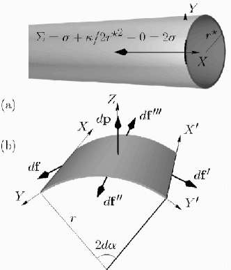
Figure 3: (a) Elastic force $\Sigma$ per unit length exerted at the extremity of a tubule with equilibrium radius $r^{\star}=\sqrt{\kappa/(2\sigma)}$. (b). Scheme of the forces involved in the calculation of the equilibrium radius of a tubule under pressure, using the Laplace law formalism with the stress tensor.

Obviously, the stress tensor should give the answer. Consider a cut along the membrane surface, perpendicular to the tube axis $X$, as depicted in Fig. 3a. From Eq. (28), we obtain for the tangential stress

$$\Sigma\equiv\Sigma_{XX}=\sigma+\frac{\kappa}{2}\times\left(\frac{1}{r^{\star}}\right)^{2}-\frac{\kappa}{2}\times 0=2\sigma$$ (44)

Note that the stress across a cut parallel to the tube axis vanishes: $\Sigma_{YY}=\sigma-\frac{1}{2}\kappa/{r^{\star}}^{2}=0$.

It is interesting to see that the equilibrium tube radius can be deduced from a generalized Laplace law. Assume that there is a pressure difference $P$ across the membrane and consider a small patch of the tube limited by four infinitesimal cuts along the principal curvature directions (fig. 3b). The force along the $Z$ direction is $dp=P\,2rd\alpha\,dX$. Clearly, the forces $d\mathbf{f}^{\prime\prime}$ and $d\mathbf{f}^{\prime\prime\prime}$ have no projection along $Z$. The contribution of the forces $d\mathbf{f}$ and $d\mathbf{f}^{\prime}$ along $Z$ gives $P\,2rd\alpha\,dX=\Sigma_{YY}dX\,d\alpha+\Sigma_{Y^{\prime}Y^{\prime}}dX\,d\alpha$, yielding

$$P=\frac{\frac{1}{2}\left(\Sigma_{YY}+\Sigma_{Y^{\prime}Y^{\prime}}\right)}{r}\,.$$ (45)

Note that it is because the total curvature $C$ is uniform that the normal components, e.g. $\Sigma_{ZX}$, do not contribute. Since $\Sigma_{YY}=\Sigma_{Y^{\prime}Y^{\prime}}=\sigma-\frac{1}{2}\kappa/r^{2}$, we obtain the equilibrium (Laplace) relation:

$$P=\frac{\sigma}{r}-\frac{\kappa}{2r^{3}}\,.$$ (46)

This equation gives the correct equilibrium radius of the tube, as would be obtained from minimizing $F=2\pi rL(\sigma+\frac{1}{2}\kappa/r^{2})-P\pi r^{2}L$ with respect to $r$. We also obviously recover $r=r^{\star}$ when $P=0$.

3.2 Adhesion and contact curvature

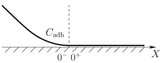
Figure 4: Membrane adhering onto a substrate. In the region $X>0$, the membrane is flat and subject to the short-range potential $W(h)=-W_{\mathrm{adh}}$. In the limit where the adhesion potential is infinitely short-ranged, the membrane departs tangentially in $X=0^{-}$ with a curvature discontinuity $C_{\mathrm{adh}}$.

With the help of the stress tensor it is immediate to recover the contact-curvature condition at the detachment point of an adhering membrane [7, 11]. Let us place ourselves in the local tangent frame at the detachment point $X=0$ (Fig. 4). For the sake of simplicity, we assume that the geometry is invariant in the $Y$ direction, that the substrate is flat and that the adhesion takes place very abruptly in $X=0$. The tangential component $\Sigma_{XX}$ of the stress tensor is given by (40). In $X=0^{+}$, the membrane is flat ($C_{X}=C_{Y}=0$) and $W(\left.h\right|_{0^{+}})=-W_{\mathrm{adh}}$, where $W_{\mathrm{adh}}$ is the adhesion energy. Hence,

$$\left.\Sigma_{XX}\right|_{0^{+}}=\sigma-W_{\mathrm{adh}}\,,$$ (47)

In $X=0^{-}$, the membrane is still parallel to the substrate but it is detached and curved with the contact-curvature $C_{X}=C_{\mathrm{adh}}$. Assuming the limit of an infinitely short-ranged potential, we may consider that $W(\left.h\right|_{0^{-}})=0$. Hence,

$$\left.\Sigma_{XX}\right|_{0^{-}}=\sigma-\frac{\kappa}{2}C_{\mathrm{adh}}^{2}\,,$$ (48)

The continuity of the tangential stress $\Sigma_{XX}$ yields then the contact-curvature condition

$$C_{\mathrm{adh}}=\sqrt{\frac{2W_{\mathrm{adh}}}{\kappa}}\,.$$ (49)

3.3 Torque balance at the boundary between domains

Vesicles made with different lipidic components may phase separate into coexisting membrane domains [12, 13, 14]. The variational problem associated with the determination of the equilibrium shape of a biphasic vesicule (even axisymmetric) is a difficult one, requiring the introduction of Lagrange multiplier fields; however, it yields a quite simple boundary conditions [12]. Here we show that this boundary condition may quite generally (and very easily) be obtained from the continuity of the torque tensor.

Consider an axisymmetric vesicle having a circular boundary separating a phase with elastic constants $\{\kappa_{1}$, $\bar{\kappa}_{1}\}$ from a phase with elastic constants $\{\kappa_{2}$, $\bar{\kappa}_{2}\}$. We place ourselves in the tangent frame $(X,Y)$ at a point along the boundary, with $X$ normal to the boundary and pointing towards phase 1 (see Fig. 5). We define also the frame with opposite directions $(X^{\prime},Y^{\prime})$. By symmetry, the axes $X$, $X^{\prime}$, $Y$ and $Y^{\prime}$ are parallel to the principal curvature directions. Let $C_{1}$ (resp. $C_{2}$) be the curvature of phase 1 (resp. 2) along $X$ (resp. $X^{\prime}$) and let $C$ be the common curvature of phases 1 and 2 along either $Y$ or $Y^{\prime}$. Then, from Eqs. (32), we obtain

$$\frac{d\bm{\tau}^{1\to 2}}{d\ell} = T_{YX}^{(1)}\,\mathbf{e}_{Y}\,=\,\left[-\kappa_{1}\left(C_{1}+C\right)-\bar{\kappa}_{1}\,C\right]\mathbf{e}_{Y},$$ (50)

$$\frac{d\bm{\tau}^{2\to 1}}{d\ell} = T_{Y^{\prime}X^{\prime}}^{(1)}\,\mathbf{e}_{Y^{\prime}}\,=\,\left[-\kappa_{2}\left(C_{2}+C\right)-\bar{\kappa}_{2}\,C\right]\mathbf{e}_{Y^{\prime}},\qquad$$ (51)

where $d\bm{\tau}^{1\to 2}$ and $d\bm{\tau}^{1\to 2}$ are the elementary torques exchanged through a cut of length $d\ell$ along the boundary. At equilibrium these two torques must balance, i.e. $d\bm{\tau}^{1\to 2}+d\bm{\tau}^{2\to 1}=0$. This yields

$$\kappa_{2}\,C_{2}-\kappa_{1}\,C_{1}=\left(\kappa_{1}+\bar{\kappa}_{1}-\kappa_{2}-\bar{\kappa}_{2}\right)C\,,$$ (52)

which is precisely the boundary condition (A22) established in the appendix of Ref. [12].

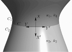
Figure 5: Region near the phase separation line in an axisymmetric biphasic vesicle. Geometry and notations used in the expression of the torque balance through the separation line.

4 Summary

The principal aim of this paper is to make it straightforward for scientists working in the field of membranes to use stress and torque concepts (instead of systematic energy minimization). To this end, from the standard Helfrich elasticity, we have derived the stress and torque tensors in a simple manner yielding explicit formulas. We have derived the expressions of the stress and torque tensors both with respect to a fixed “projected” frame and in the local tangent frame. Although we have restricted our calculations to small deformations with respect to a flat shape, our results are compatible with the fully covariant results of Ref. [4]: this is because one may always work locally in the tangent plane and because the Helfrich energy is only quadratic in the curvature. We have included the contribution arising from the Gaussian rigidity, which is always present and cortributes to the torque tensor; we have included the contribution from a possible surface adhesion potential. We have shown several examples where the direct use of stress and torque concepts is very fruitful.

Stimulating discussions with P. Sens, at the origin of this work, are gratefully acknowledged. The author also thanks J.-F. Joanny for enlightening discussions.

References

- [1] O. G. Mouritsen, Life—as a matter of fat (The frontiers collection, Springer, Berlin, 2005).
- [2] B. Alberts, A. Johnson, J. Lewis, M. Raff, K. Roberts, P. Walter, Molecular Biology of the Cell (Garland, New York, 2002), 4th ed.
- [3] W. Helfrich, Z. Naturforsch., 1973, C 28, 693.
- [4] R. Capovilla and J. Guven, J. Phys. A, 2002, 35, 6233.
- [5] M. M. Müller, M. Deserno and J. Guven, Europhys. Lett., 2005, 69 (3), 482.
- [6] E. E. Evans, Biophys. J., 1985, 48, 175.
- [7] U. Seifert and R. Lipowsky, Phys. Rev. A, 1990, 42, 4768.
- [8] U. Seifert and R. Lipowsky, in Dynamical phenomena at surfaces, interfaces and membranes ed. by D. Beysens, N. Boccara and G. Forgacs (Nova Science Publishers, Commack, 1993), 295–304.
- [9] I. Derényi and F. Jülicher and J. Prost, Phys. Rev. Lett., 2002, 88, 238101.
- [10] T. R. Powers and G. Huber and R. E. Goldstein, Phys. Rev. E, 2002, 65, 041901.
- [11] R. Capovilla and J. Guven, Phys. Rev. E, 2002, 66, 041604.
- [12] F. Jülicher and R. Lipowsky, Phys. Rev. E, 1996, 53, 2670.
- [13] T. Baumgart, S. T. Hess and W. W. Webb, Nature, 2003, 425, 821.
- [14] J.-M. Allain, C. Storm, A. Roux, M. Ben Amar and J.-F. Joanny, Phys. Rev. Lett., 2004, 93, 158104.