Anisotropy and Order of Epitaxial Self-Assembled Quantum Dots

Abstract

Epitaxial self-assembled quantum dots (SAQDs) represent an important step in the advancement of semiconductor fabrication at the nanoscale that will allow breakthroughs in electronics and optoelectronics. In these applications, order is a key factor. Here, the role of crystal anisotropy in promoting order during early stages of SAQD formation is studied through a linear analysis of a commonly used surface evolution model. Elastic anisotropy is used a specific example. It is found that there are two relevant and predictable correlation lengths. One of them is related to crystal anisotropy and is crucial for determining SAQD order. Furthermore, if a wetting potential is included in the model, it is found that SAQD order is enhanced when the deposited film is allowed to evolve at heights near the critical surface height for three-dimensional film growth.

Epitaxial self-assembled quantum dots (SAQDs) represent an important step in the advancement of semiconductor fabrication at the nanoscale that will allow breakthroughs in electronics and optoelectronics. SAQDs are the result of linearly unstable film growth in strained heteroepitaxial systems such as $\mbox{Si}_{x}$$\mbox{Ge}_{1-x}$/Si and $\mbox{In}_{x}\mbox{Ga}_{1-x}\mbox{As}$/GaAs and other systems. SAQDs have great potential for electronic and optoelectronic applications. In these applications, order is a key factor. There are two types of order, spatial and size. Spatial order refers to the regularity of SAQD dot placement, and it is necessary for nano-circuitry applications. Size order refers to the uniformity of SAQD size which determines the voltage and/or energy level quantization of SAQDs. It has been observed that crystal anisotropy can have a beneficial effect on SAQD order. Liu:2003kx Here, the role of crystal anisotropy in promoting order during early stages of SAQD formation is studied through a linear analysis of a commonly used surface evolution model. Spencer:1993vt ; Liu:2003kx ; Zhang:2003tg ; Tekalign:2004jh ; Friedman:2006bc

The linear analysis addresses the initial stages of SAQD formation when the nominally flat film surface becomes unstable and transitions to three-dimensional growth. This early stage of SAQD growth determines the initial seeds of order or disorder in an SAQD array, and can be analyzed analytically. A dispersion relation as in Spencer:1993vt ; Golovin:2003ms is used, and two predictable correlation lengths that grow as the square-root of time (Eqs. 14 and 17) are found. One of the correlation lengths results from crystal anisotropy. This length plays a limiting role in the initial order of SAQD arrays, and it is shown that anisotropy is crucial for creating a lattice-like structure that is most technologically useful. This method of analysis can be extended for use in any “nucleationless” model of SAQD growth, although here, the specific instance of elastic anisotropy is treated as elastic anisotropy is the most easily estimated. Anisotropy of surface energy may also effect SAQD order, and a similar analysis would result.

At later stages when surface fluctuations are large, non-linear dynamics come into play. At this stage, there is a natural tendency of SAQDS to either order or ripen. Golovin:2003ms ; Liu:2003kx Ripening systems will tend to have increased disorder as time progresses, while ordering systems will tend to order only slightly due to critical slowing down. Wang:2004dd Also, it is important to note that while an ordering system might be “ordered” when compared to other non-linear phenomena such as convection roles, etc. Cross:1993ti , the requirements for technological application are much more stringent. In a numerical investigation, it was found that SAQDs have enhanced order due to crystal anisotropy, but soon become disordered from ripening. Liu:2003kx In any case, an understanding of the order during the initial stages of SAQD growth is essential to further investigation of the final SAQD array order.

As in Zhang:2003tg ; Golovin:2003ms ; Liu:2003kx ; Spencer:1993vt , a wetting energy is included in the analysis. The wetting potential ensures that growth takes place in the Stranski-Krastanow mode: a 3D unstable growth occurs only after a critical layer thickness is achieved, and a residual wetting layer persists. Although somewhat controversial, the physical origins and consequences of the wetting potential are discussed in Beck:2004yq ; Spencer:1993vt . The analysis presented here is quite general, and one can exclude or neglect the effect of the wetting potential by simply setting it to zero. That said, if the wetting potential is real, the present analysis shows that it beneficial to SAQD order to grow near the critical layer thickness.

The remainder of this report is organized as follows. First, stochastic initial conditions are discussed. Second, the evolution of a single mode for the isotropic case is discussed. Third, the resulting correlation functions and correlation lengths are derived for the isotropic case. Fourth, the analysis is repeated for the anisotropic case using elastic anisotropy as an example. Finally, a representative numerical example is presented using parameters appropriate for Ge dots grown on Si.

To analyze resulting SAQD order, the mathematical model must include stochastic effects. For simplicity, stochastic initial conditions with deterministic time evolution are used. This method of analysis yields a correlation function that is used to characterize SAQD order.

In this model, the film height $0pt$ is a function of lateral position $\mathbf{x}$ and time $t$. The film height is treated as an average film height ($\bar{0pt}$) with surface fluctuations $h(\mathbf{x},t)$ ,

$$\mathcal{H}=\bar{\mathcal{H}}+h(\mathbf{x},t).$$ (1)

In this way, $\bar{0pt}$ functions as a control parameterCross:1993ti physically signifying the amount of available material per unit area to form SAQDs, and $h(\mathbf{x},t)$ evolves via surface diffusion giving the the resulting surface profile. Order is then analyzed using using the spatial correlation function, $\left\langle h(\mathbf{x},t)h(\mathbf{0},t)\right\rangle$ and the corresponding spectrum function $\left\langle h_{\mathbf{k}}(t)h_{\mathbf{k}^{\prime}}(t)^{*}\right\rangle$.

An initially flat surface is in unstable equilibrium, and it is necessary to perturb it to produce SAQDs. Therefore, stochastic initial conditions are implemented by letting $h(\mathbf{x},0)$ in Eq. 1 be random white noise. Specifically, $h(\mathbf{x},0)$ is assumed to be sampled from a normal distribution such that

$$\left\langle h(\mathbf{x},0)\right\rangle=0\mbox{, and }\left\langle h(\mathbf{x},0)h(\mathbf{x}^{\prime},0)\right\rangle=\Delta^{2}\delta^{d}\left(\mathbf{x}-\mathbf{x}^{\prime}\right)$$ (2)

where $\Delta$ is the noise amplitude of dimension [length]^1+d/2, $d$ is the dimension of the surface, and $\delta^{d}(\mathbf{x})$ is the $d\mbox{-dimensional}$ Dirac Delta function. Much of the following analysis uses the Fourier transform with the convention, $h_{\mathbf{k}}(t)=(2\pi)^{-d}\int d^{d}\mathbf{k}\,\exp(-i\mathbf{k}\cdot\mathbf{x})h(\mathbf{x},t).$ The mean and two-point correlation functions for $h_{\mathbf{k}}(0)$ are

$$\left\langle h_{\mathbf{k}}(0)\right\rangle=0\mbox{, and }\left\langle h_{\mathbf{k}}(0)h_{\mathbf{k}^{\prime}}(0)^{*}\right\rangle=\frac{\Delta^{2}}{(2\pi)^{d}}\delta^{d}\left(\mathbf{k}-\mathbf{k}^{\prime}\right).$$ (3)

The deterministic evolution of a single Fourier component is determined by surface diffusion with a diffusion potential $\mu(\mathbf{x},t)$.Zhang:2003tg ; Spencer:1993vt This model is phenomenological in nature, but contains the essential elements of SAQD formation. Thus, it is an adequate, but not overly complex starting point for the investigation of the effects of crystal anisotropy. Furthermore, models of this nature can be derived from atomic scale simulations. Haselwandter:2006hy At any instant in time, the growing film is described by the curve $\mathcal{H}(\mathbf{x},t)$. Using Eq. 1 to decompose the film height,

$$\partial_{t}h(\mathbf{x},t) = \mathbf{\nabla}\cdot(\mathcal{D}\mathbf{\nabla}\mu(\mathbf{x},t;\bar{0pt}));$$

$$d\bar{0pt}/dt = Q,$$

where $\mu$ depends on $\bar{0pt}$, and $Q$ is the flux of new material onto the surface.

The appropriate diffusion potential $\mu$ must produce Stranski-Krastanow growth. Thus, it must incorporate the elastic strain energy density $\omega$ that destabilizes a planar surface, the surface energy density $\gamma$ that stabilizes planar growth and a wetting potential $W(\mathcal{H})$ that ensures substrate wetting. The simplest form that gives the appropriate behavior is

$$\mu=\Omega\left(\omega-\kappa\gamma+n_{z}W^{\prime}(0pt)\right)$$ (4)

similar to Liu:2003kx ; Golovin:2003ms ; Tekalign:2004jh ; Friedman:2006bc where $\Omega$ is the atomic volume, $\kappa$ is the total surface curvature, and $n_{z}$ is the vertical component of the unit surface normal $\hat{n}$. The strain energy density $\omega$ is found using isotropic linear plane strain elasticity. In general, $\omega$ is a function of $x$, and it is a non-local functional of the entire surface profile $\mathcal{H}(x)$.

Consider first, the the one-dimensional and two-dimensional isotropic cases. Following Golovin:2003ms ; Spencer:1993vt ; Tekalign:2004jh , the surface diffusion potential, (Eq. 4) is expanded to first order in the film height fluctuation $h$. The elastic energy $\omega$ is calculated using linear isotropic elasticity. It is a non-local function of $h(\mathbf{x})$; thus, it is useful to work with the Fourier transform. In the isotropic case, the linearized diffusion potential (Eq. 5) depends only on the wave vector magnitude $k=\left\|\mathbf{k}\right\|$ . Thus,

$$\mu_{\mathbf{k}} = f(k,\bar{0pt})h_{\mathbf{k}},\mbox{ with}$$ (5)

$$f(k,\bar{0pt}) = \Omega\left(-2M(1+\nu)\epsilon_{0}^{2}k+\gamma k^{2}+W^{\prime\prime}(\bar{0pt})\right).$$ (6)

In the anisotropic case, there will also be a dependence on the wave vector direction $\theta_{\mathbf{k}}$.

The time dependence of the film height has a simple solution if there is no additional flux of material ($Q=0$, and $\bar{0pt}$ is constant).

$$h_{\mathbf{k}}(t) = h_{\mathbf{k}}(0)e^{\sigma_{k}t}\mbox{, with}$$ (7)

$$\sigma_{k} = -\mathcal{D}k^{2}f(k,\bar{0pt}),$$ (8)

where $\sigma_{k}$ is the dispersion relation and depends only on the wavevector magnitude $k$. Modes with positive $\sigma_{k}$ are grow unstably, while modes with negative values of $\sigma_{k}$ decay.

The important features of $\sigma_{k}$ are most easily recognized using a characteristic wavenumber is $k_{c}=2M(1+\nu)\epsilon_{0}^{2}/\gamma$ and a characteristic time $t_{c}=(\mathcal{D}\Omega\gamma k_{c}^{4})^{-1}$. Spencer:1993vt ; Golovin:2003ms

$$\sigma_{k}=t_{c}^{-1}\alpha^{2}(\alpha-\alpha^{2}-\beta).$$ (9)

where the shorthand $\alpha=k/k_{c}$ and $\beta=W^{\prime\prime}(\bar{0pt})/(\gamma k_{c}^{2})$ is used.

The dispersion relation (Eq. 9) has a peak at $k_{0}=\alpha_{0}k_{c}$ where

$$\alpha_{0}=\frac{1}{8}\left(3+\sqrt{9-32\beta}\right).$$

Expanding $\sigma_{k}$ about $k_{0}$,

$$\sigma_{k}\approx\sigma_{0}-\frac{1}{2}\sigma_{2}\left(k-k_{0}\right)^{2}\mbox{ where }$$

$$\sigma_{0}=\frac{1}{4t_{c}}\alpha_{0}^{2}\left(\alpha_{0}-2\beta\right),\quad\sigma_{2}=k_{c}^{-2}t_{c}^{-1}(3\alpha_{0}-4\beta).$$ (10)

Thus,

$$h_{\mathbf{k}}(t)\approx h_{\mathbf{k}}(0)e^{\sigma_{0}t-\frac{1}{2}\sigma_{2}t\left(k-k_{0}\right)^{2}}.$$ (11)

Now, the statistical correlation functions and correlation lengths that characterize order are derived. Using Eqs. 7 and 11 along with the stochastic initial conditions (Eqs. 2 and 3) , the mean value of $h_{\mathbf{k}}(t)$ is

$$\left\langle h_{\mathbf{k}}(t)\right\rangle=\left\langle h_{\mathbf{k}}(0)\right\rangle e^{\sigma_{k}t}=0,$$

so that the mean surface perturbation is simply $0$ for all time and all $\mathbf{k}$. However, the mean-square surface perturbations as characterize by the second-order correlation function Zwanzig:2001zf can be large,

$$\left\langle h_{\mathbf{k}}(t)h_{\mathbf{k}^{\prime}}(t)^{*}\right\rangle = \left\langle h_{\mathbf{k}}(0)h_{\mathbf{k}^{\prime}}(0)^{*}\right\rangle e^{(\sigma_{k}+\sigma_{k^{\prime}})t}$$ (12)

$$= \frac{\Delta^{2}}{(2\pi)^{d}}\delta^{d}\left(\mathbf{k}-\mathbf{k^{\prime}}\right)e^{2\sigma_{k}t},$$

using Eq. 3. The real space correlation function can be found by taking the inverse Fourier transform of Eq. 12,

$$\left\langle h(\mathbf{x},t)h(\mathbf{x}^{\prime},t)^{*}\right\rangle = \int d^{d}\mathbf{k}\int d^{d}\mathbf{k}^{\prime}\,e^{i\mathbf{k}\cdot\mathbf{x}-i\mathbf{k}^{\prime}\cdot\mathbf{x}^{\prime}}\left\langle h_{\mathbf{k}}(t)h_{\mathbf{k}^{\prime}}(t)^{*}\right\rangle$$ (13)

$$= \frac{\Delta^{2}}{(2\pi)^{d}}\int d^{d}\mathbf{k}\,e^{i\mathbf{k}\cdot\left(\mathbf{x}-\mathbf{x}^{\prime}\right)}e^{2\sigma_{k}t}$$

where integration over $\mathbf{k}^{\prime}$ is simple due to the $\delta^{d}\left(\mathbf{k}-\mathbf{k^{\prime}}\right)$ in Eq. 12.

Using Eq. 10,

$$e^{2\sigma_{k}t}\approx e^{2\sigma_{0}t-\frac{1}{2}(2\sigma_{2}t)(k-k_{0}^{2})}$$

which is peaked at $k=k_{0}$. This form suggests that the real-space correlation function is periodic with a gaussian envelope that has a standard deviation of

$$L_{cor}=\sqrt{2\sigma_{2}t}$$ (14)

$L_{cor}$ is the correlation length of the film-height profile, and characterizes the degree of order of the SAQD array. For example, in one dimension ($d=1)$,

$$\left\langle h(x,t)h(0,t)^{*}\right\rangle\dots$$

$$\dots=\frac{\Delta^{2}}{2\pi}\sum_{\pm}\int_{0}^{\infty}dk\,e^{2\sigma_{0}t-\frac{1}{2}L_{cor}^{2}(k-k_{0})^{2}\pm ikx}$$

$$\dots\approx\frac{2\Delta^{2}}{(2\pi L_{cor}^{2})^{1/2}}e^{2\sigma_{0}t-\frac{1}{2}(x/L_{cor})^{2}}\cos(k_{0}x)$$

an approximation that is valid if $k_{c}L_{cor}\gg 1$. Thus, $L_{cor}$ gives the length scale over which dots will be ordered, and this scale grows as $t^{1/2}$. As $t\rightarrow\infty$,

$$\left\langle h(x,t)h(0,t)^{*}\right\rangle=\frac{2\Delta^{2}}{(2\pi L_{cor}^{2})^{1/2}}e^{2\sigma_{0}t}\cos(k_{0}x),$$

and the entire array should be perfectly ordered.

The situation in two-dimensions, however, is less friendly. As $t\rightarrow\infty$, $L_{cor}\rightarrow\infty$, and $e^{-\frac{1}{2}L_{cor}^{2}(k-k_{0})}\approx(2\pi/L_{cor}^{2})^{1/2}\delta(k-k_{0})$

$$\left\langle h(\mathbf{x},t)h(\mathbf{0},t)^{*}\right\rangle\dots$$

$$\dots=\frac{\Delta^{2}}{(2\pi)^{3/2}L_{cor}}\int d^{2}\mathbf{k}\,e^{2\sigma_{0}t+i\mathbf{k}\cdot\mathbf{x}}\delta(k-k_{0})$$

$$\dots=\frac{\Delta^{2}k_{0}}{(2\pi L_{cor}^{2})^{1/2}}e^{2\sigma_{0}t}J_{0}(k_{0}\parallel\mathbf{x}\parallel)$$

Thus, the two-dimensional isotropic case has statistical order at large times, but does not yield SAQD lattices as does the one-dimensional case (see Fig. 1a and b).

Now, consider the effects of crystal anisotropy. For example, let the elastic energy term $\omega$ have $N$-fold symmetry while the other terms are assumed isotropic. Then, the growth rate depends on the both the wave vector magnitude $k$ (and thus on $\alpha=k/k_{c}$) and direction $\theta_{\mathbf{k}}$ so that, $\sigma_{k}\rightarrow\sigma_{\mathbf{k}}$. Naturally, the anisotropic elastic energy term in the growth rate $\sigma_{\mathbf{k}}$ depends on the specific anisotropic elastic constants, but the general qualitative effect of elastic anisotropy on SAQD growth kinetics can be investigated without incorporating a detailed elastic calculation at this time. Thus, the present work provides motivation for more detailed calculation. A reasonable way to estimate how the elastic energy term varies with direction ($\theta_{\mathbf{k}}$) is to assume a low order harmonic form with the proper rotational symmetry. The simplest such guess is

$$\sigma_{\mathbf{k}} = t_{c}^{-1}\alpha^{2}\left(\alpha\left(1-\epsilon\sin^{2}\left(N\theta_{\mathbf{k}}/2\right)\right)-\alpha^{2}-\beta\right),$$

where $\epsilon$ parameterizes the importance of the directional-dependence. More precise calculations using anisotropic elastic constants of real materials (similar to ref. Obayashi:1998fk ) will be given in future work.

$\sigma_{\mathbf{k}}$ has peaks at $N$ wave vectors,

$$\mathbf{k}_{n}=k_{0}\left(\left(\cos\theta_{n}\right)\hat{e}_{x}+\left(\sin\theta_{n}\right)\hat{e}_{y}\right)$$

with $\theta_{n}=2\pi(n-1)/N$. Around each peak, $\mathbf{k}$ can be decomposed in the direction parallel ($k_{\parallel})$ and perpendicular ($k_{\perp}$) to $\mathbf{k}_{n}$. Using this decomposition and expanding $e^{2\sigma_{\mathbf{k}}t}$ about each peak,

$$e^{2\sigma_{\mathbf{k}}t}\approx\sum_{n=1}^{N}\exp\left(2\sigma_{n}t\right);$$ (15)

$$2\sigma_{n}t=2\sigma_{0}t-\frac{1}{2}L_{\parallel}^{2}(k_{\parallel}-\alpha_{0}k_{c})^{2}-\frac{1}{2}L_{\perp}^{2}k_{\perp}^{2};$$ (16)

$$L_{\parallel}=\sqrt{2\sigma_{2}t},\mbox{ and }L_{\perp}=\sqrt{(N^{2}\alpha_{0}\epsilon t_{c}^{-1}k_{c}^{-2})t}.$$ (17)

Note that $L_{\parallel}$ is the same as $L_{cor}$ for the isotropic case. Eq. 15 is valid if $k_{c}L_{\parallel}\gg 1,\mbox{ and }k_{c}L_{\perp}\gg 1$. Using, Eq. 13, but noting that $\sigma_{\mathbf{k}}$ now depends on both the magnitude and direction of $\mathbf{k}$, along with Eqs. 15, and 16,

$$\left\langle h(\mathbf{x},t)h(\mathbf{0},t)^{*}\right\rangle=\frac{\Delta^{2}}{(2\pi)^{2}}\frac{2\pi}{L_{\parallel}L_{\perp}}\dots$$

$$\dots\sum_{n=1}^{N/2}e^{2\sigma_{0}t-\frac{1}{2}\left(L_{\parallel}^{-2}x_{\parallel}^{2}+L_{\perp}^{-2}x_{\perp}^{2}\right)}2\cos\left(k_{0}x_{\parallel}\right),$$ (18)

where $x_{\parallel}=(\cos\theta_{n})x+(\sin\theta_{n})y$, and $x_{\perp}=(-\sin\theta_{n})x+(\cos\theta_{n})y$. Thus, the same tendency to long-range order as for the one-dimensional case is present (see Fig. 1c and d).

As a numerical example, consider Ge grown on Si. Both the isotropic approximation and an estimated elastically anisotropic case (with $N=4$, and $\epsilon=0.1$) are treated. Neglecting the difference in elastic properties of the Si substrate, $E_{\text{Ge}}=1.361\times 10^{12}\mbox{ dyne/cm}^{2}$, $\nu_{\text{Ge}}=0.198$, $\epsilon_{0}=-0.0418$, $\Omega=2.27\times 10^{-23}\mbox{cm}^{3}$, $\gamma=1927\mbox{ erg/cm}^{2}$, and $W(0pt)=4.75\times 10^{-6}/0pt\mbox{ erg/cm}^{3}$. The resulting biaxial modulus is $M=1.697\times 10^{12}\text{ dyne/cm}^{2}$, characteristic wavenumber is $k_{c}=0.369\text{ nm}^{-1}$ and critical film height is $\bar{0pt}_{c}=1.132\text{ nm}\approx 4\mbox{ ML}$. If the film is grown to a thickness of $\bar{0pt}=0pt_{c}+0.25\mbox{ ML}\approx 1.203\text{ nm}$, and then allowed to evolve, $\beta=0.2078$, $\alpha_{0}=0.5664$, $k_{0}=0.209\text{ nm}^{-1}$, $\sigma_{0}=0.01206t_{c}^{-1}$, $\sigma_{2}=0.867k_{c}^{-2}t_{c}^{-1}$, $L_{\parallel}=0.746k_{0}^{-1}(t/t_{c})^{1/2}$, and $L_{\perp}=0.539k_{0}^{-1}(t/t_{c})^{1/2}$. Note that the unspecified diffusivity $\mathcal{D}$ has been absorbed into $t_{c}$. The film will stay in the linear regime as long as the surface fluctuations stay small. For this purpose, let “small” mean $1\mbox{ ML}=2.83\times 10^{-8}\mbox{cm}$. Once the fluctuations become “large”, individual dots will begin to form, and a nonlinear analysis becomes necessary. It is useful to know the correlation lengths at this time.

To find the correlation lengths, one must choose the initial height fluctuation intensity $\Delta$ and then calculate the time for fluctuations to become “large”. The initial fluctuation intensity is somewhat arbitrary, but $\Delta=8.02\times 10^{-16}\mbox{ cm}^{2}$ gives an average fluctuation of $1\mbox{ ML}$ over a patch $1\mbox{ ML}^{2}$ and seems appropriate. Next Eqs. 17 and 18 are used to find $t$ for which the r.m.s. fluctuations become large $h_{rms}=\left\langle|h(0,t)|^{2}\right\rangle^{1/2}=a_{0}$. There are two solutions, $t/t_{c}=5.53\times 10^{-3}$, and $t/t_{c}=471$. The first solution is an artifact of the white noise initial conditions and occurs during an initial shrinking of the surface height variance; thus, the second solution is taken. At $t/t_{c}=471$, the correlation lengths are found using Eq. 17, $L_{cor}=L_{\parallel}=77.5\mbox{ nm}$, and $L_{\perp}=56.0\mbox{ nm}$. The smaller correlation length gives $k_{0}L_{\perp}/\pi=3.73$, so a patch of about 4 dots across is expected to be reasonably well ordered.

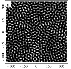
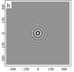
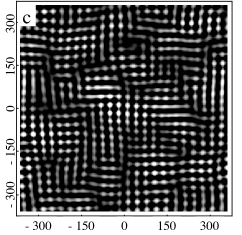
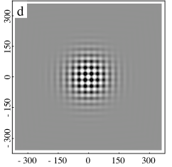
Figure 1: Density plots of surface profiles and correlation functions at $t/t_{c}=471.$ The scale is in nm, and the physical parameters are listed in the text. Plots (a) and (b) are a sample surface profile and correlation function respectively for an elastically isotropic material. Plots (c) and (d) are a surface profile and correlation function for an elastically anisotropic material with 4-fold symmetry. Surface profile plots saturate black at a minimum of $0pt=\bar{0pt}$ for clarity. White dots indicate surface peaks. Correlation function plots span $\pm$ the maximum value / 2.

A numerical simulation of linear size $l=24(2\pi/k_{0})=722\text{ nm}$ can be easily performed. The discrete initial conditions $h_{\mathbf{k}}$(0) are taken from a normal distribution of zero mean and variance $\left\langle h_{\mathbf{k}}(0)h_{\mathbf{k}^{\prime}}^{*}(0)\right\rangle_{discrete}=(\Delta^{2}/l^{2})\delta_{\mathbf{k}\mathbf{k}^{\prime}}$, where $\delta_{\mathbf{k}\mathbf{k}^{\prime}}$ is the Kronecker delta, and each vector component of $\mathbf{k}$ takes discrete values $2\pi m/l$ with $m$ an integer. These components then evolve via Eq. 7. The results of an isotropic and anisotropic simulation along with the corresponding real-space correlation functions are shown in Fig. 1. These plots clearly demonstrate the importance of anisotropy in producing long range order.

Figs. and 1c and d appear to agree qualitatively with observations of nucleationless growth of Ge_xSi_1-x nanostructures on Si Berbezier:2003mw ; Brunner:2002gf ; Gao:1999ve , although mostly with $x<0.5$. Typical observed dot arrangements appear to correspond to lower values of $\beta$ than 0.2078 used for the example as they are quasiperiodic but less ordered than Fig. 1c. Quantitative reporting of correlation lengths would assist comparison and possibly enable better tuning of phenomenological models to experiments. InP/InGaP nanostructures reported in Bortoleto:2003zh appear similar.

From the analysis of the isotropic model, it is clear that long range statistical order (long correlation lengths) require tight distributions in reciprocal space. This long range statistical order is achieved in the large time limit, but this statistical order is insufficient to produce a well-ordered array of SAQDs. This lack of usable order is reflected in the real-space two-point correlation function of the isotropic model. However, in the one-dimensional and two-dimensional anisotropic cases, there is tendency to form a lattice after a long time. In the anisotropic case, there are two correlation lengths that characterize observed SAQD array order. Analytic formulas for these correlation lengths have been given for a model with elastic simplified anisotropy, but the general conclusions and method of analysis should apply to any source of anisotropy. Additionally, from a simple form of the wetting potential it is observed that at film heights just above the critical threshold $0pt_{c}$, the correlation lengths can grow quickly while the height fluctuations grow slowly; thus order is enhanced. Availability of measured SAQD correlation lengths would help to improve this analysis and to engineer more ordered quantum dot arrays.

References

- (1) P. Liu, Y. W. Zhang, C. Lu. Phys. Rev. B, 67:165414, 2003.
- (2) B. J. Spencer, P. W. Voorhees, S. H. Davis. J. Appl. Phys., 73(10):4955–4970, 1993.
- (3) Y.W. Zhang, A.F. Bower, P. Liu. Thin solid films, 424:9–14, 2003.
- (4) W. T. Tekalign, B. J. Spencer. J. Appl. Phys., 96(10):5505–5512, 2004.
- (5) Lawrence H. Friedman, Jian Xu. Appl. Phys. Lett., 88:093105, 2006.
- (6) A. A. Golovin, S. H. Davis, P. W. Voorhees. Phys. Rev. E, 68:056203, 2003.
- (7) Yu U. Wang, Yongmei M. Jin, Armen G. Khachaturyan. Acta Mater., 52:81–92, 2004.
- (8) M. C. Cross, P. C. Hohenberg. Rev. Mod. Phys., 65(3):851–1112, 1993.
- (9) M. J. Beck, A. van de Walle, M. Asta. Phys. Rev. B, 70(20):205337, Nov 2004.
- (10) C. Haselwandter, D VVedensky. 2006 APS March Meeting, 2006.
- (11) Robert Zwanzig. Nonequilbrium Statistical Mechanics. Oxford University Press, New York, 2001.
- (12) Y. Obayashi, K. Shintani. J. Appl. Phys., 84(6):3141, 1998.
- (13) I. Berbezier, A. Ronda, F. Volpi, A. Portavoce. Surf. Sci., 531:231–243, 2003.
- (14) Karl Brunner. Rep. Prog. Phys., 65(1):27–72, 2002.
- (15) H. J. Gao, W. D. Nix. Annu. Rev. Mater. Sci., 29:173–209, 1999.
- (16) J. R. R. Bortoleto, H. R. Gutierrez, M. A. Cotta, J. Bettini, L. P. Cardoso, M. M. G. de Carvalho. Appl. Phys. Lett., 82(20):3523–3525, 2003.