Exciton-exciton scattering :
Composite boson versus elementary boson

Abstract

This paper shows the necessity of introducing a new quantum object, the “coboson”, to properly describe any composite particle, like the exciton, which is made of two fermions. Although commonly dealed with as elementary bosons, these composite bosons — “cobosons” in short — differ from them due to their composite nature which makes the handling of their many-body effects quite different from the existing treatments valid for elementary bosons. As a direct consequence of this composite nature, there is no correct way to describe the interaction between cobosons as a potential $V$. This is rather dramatic because, with the Hamiltonian not written as $H=H_{0}+V$, all the usual approaches to many-body effects fail. In particular, the standard form of the Fermi golden rule, written in terms of $V$, cannot be used to obtain the transition rates of two cobosons. To get them, we have had to construct an unconventional expression for this Fermi golden rule in which $H$ only appears. Making use of this new expression, we here give a detailed calculation of the time evolution of two excitons. We compare the results of this exact approach with the ones obtained by using an effective bosonic Hamiltonian in which the excitons are considered as elementary bosons with effective scatterings between them, these scatterings resulting from an elaborate mapping between the two-fermion space and the ideal boson space. We show that the relation between the inverse lifetime and the sum of the transition rates for elementary bosons differs from the one of composite bosons by a factor of 1/2 ; so that it is impossible to find effective scatterings between bosonic excitons giving these two physical quantities correctly, whatever the mapping from composite bosons to elementary bosons is. The present paper thus constitutes a strong mathematical proof that, in spite of a widely spread belief, we cannot forget the composite nature of these cobosons, even in the extremely low density limit of just two excitons. This paper also shows the (unexpected) cancellation in the Born approximation of the two-exciton transition rate for a finite value of the momentum transfer.

PACS.: 71.35.-y Excitons and related phenomena

1 Introduction

Excitons are known to be composite particles made of one electron and one hole. They of course interact through the electron-electron, hole-hole and electron-hole Coulomb potentials. They also interact in a quite subtle manner, through Pauli exclusion between the fermions from which they are made. The purpose of this paper is to study how this Pauli exclusion enters the exciton transition rate and lifetime.

The major difficulty induced by the composite nature of the excitons is the impossibility to identify an interaction potential between excitons, even for the Coulomb contribution. While the electron-electron and hole-hole Coulomb potentials are unambiguously parts of the interaction between two excitons, such an identification is ambiguous for the electron-hole parts. Indeed, while $V_{eh^{\prime}}=-e^{2}/|\mathbf{r}_{e}-\mathbf{r}_{h^{\prime}}|$ is part of the interaction between excitons made of $(e,h)$ and $(e^{\prime},h^{\prime})$, the same $V_{eh^{\prime}}$ is clearly not part of the interaction between excitons if these excitons are made of $(e,h^{\prime})$ and $(e^{\prime},h)$. Since electrons and holes are indistinguishable, there is no way to know how these two excitons are made, so that there is no way to write the part of the Coulomb interaction between two excitons properly.

In spite of this obvious problem, various procedures [1,2] have been proposed to replace the semiconductor Hamiltonian written in terms of electrons and holes by an effective Hamiltonian written in terms of excitons considered as elementary bosons, with an effective exciton-exciton potential between them. Even if the bosonization procedures may appear as rather sophisticated [3], it is clear that some uncontrolled manipulations have to be done in the mapping of the two-fermion subspace into the ideal boson subspace, in order to transform the exact electron-electron Coulomb potential, written in terms of electron operators as $a^{\dagger}a^{\dagger}a\,a$, into a part of an exciton-exciton potential, which, in terms of exciton operators, reads as $B^{\dagger}B^{\dagger}B\,B$, these exciton operators being made of electron-hole pairs, i. e., $B^{\dagger}$ being linear combinations of $a^{\dagger}b^{\dagger}$. In a previous work [4], we have already shown that there is no way to find prefactors for these $B^{\dagger}B^{\dagger}B\,B$ terms which could produce the correct correlations between two excitons at any order in the exciton-exciton interaction. We here show somewhat in details that there is no way to find $B^{\dagger}B^{\dagger}B\,B$ prefactors which would produce both the exciton-exciton transition rate and the lifetime of an exciton state correctly, even in the case of just two excitons : If we know the correct value of one of these two physical quantities, for example the transition rate, we can possibly adjust the $B^{\dagger}B^{\dagger}BB$ prefactors in the effective bosonic Hamiltonian to recover the correct transition rate. However, there is no way to be sure that the same prefactors would give other physical quantities correctly, a factor of 2 being actually missed in the lifetime, as previously reported in ref. [5].

This major failure, which puts the concept of effective bosonic Hamiltonian to describe interacting excitons in a very bad shape, should push the very large amount of physicists using such effective Hamiltonians [6-14], to reconsider their works in the light of the many-body theory for “cobosons” — a contraction for composite bosons — that we have recently constructed [15] and which is free from any bosonization.

The fact that a trustworthy exciton-exciton potential does not exist, has dramatic consequences on the possible treatment of many-body effects involving excitons. Indeed, all known approaches to many-body effects [16,17] are based on rewriting the Hamiltonian as $H=H_{0}+V$, with $V$ being the interaction potential responsible for the many-body effects, and treating $V$ as a perturbation, possibly at infinite order in case of singularities. Without the availability of such a potential $V$, a novel many-body procedure, which does not rely on a would-be $V$, has thus to be constructed from scratch in order to derive many-body effects between excitons. This is the purpose of the theory we are presently developing.

In order to put the difficulty associated with the composite nature of the excitons on a proper formal basis, it is of importance to realize that all failures in the previous approaches to the exciton many-body physics can be traced back to the difficulty of properly handling Pauli exclusion, which prevents these excitons from being exact bosons. Let us introduce the exciton creation operators $B_{i}^{\dagger}$ as being such that the $B_{i}^{\dagger}|v\rangle$’s are the exact one-electron-hole-pair eigenstates of the semiconductor Hamiltonian,

$$(H-E_{i})B_{i}^{\dagger}|v\rangle=0,$$

$|v\rangle$ being the vacuum state. These operators can be expanded on the free-electron-hole-pair operators as

$$B_{i}^{\dagger}=\sum_{\mathbf{k}_{e},\mathbf{k}_{h}}\langle\mathbf{k}_{e},\mathbf{k}_{h}|i\rangle a_{\mathbf{k}_{e}}^{\dagger}\,b_{\mathbf{k}_{h}}^{\dagger}\ ,$$ (1.1)

where $a_{\mathbf{k}_{e}}^{\dagger}$ and $b_{\mathbf{k}_{h}}^{\dagger}$ are the creation operators for free electrons and free holes, with momentum $\mathbf{k}_{e}$ and $\mathbf{k}_{h}$, respectively. $\langle\mathbf{k}_{e},\mathbf{k}_{h}|i\rangle$ is the $i$ exciton wave function in momentum space, namely $\langle\mathbf{k}_{e},\mathbf{k}_{h}|i\rangle=\delta_{\mathbf{k}_{e}+\mathbf{k}_{h},\mathbf{Q}_{i}}\,\langle\alpha_{h}\mathbf{k}_{e}-\alpha_{e}\mathbf{k}_{h}|\nu_{i}\rangle$, where $\mathbf{Q}_{i}$ is the $i$ exciton center-of-mass momentum and $\langle\mathbf{k}|\nu_{i}\rangle$ is the relative motion wave function of the $i$ exciton in $\mathbf{k}$ space, with $\alpha_{e}=1-\alpha_{h}=m_{e}/(m_{e}+m_{h})$. Using eq. (1.1), it is straightforward to show that, while $[B_{i},B_{j}]=0$ as usual for bosons, the commutator $\left[B_{i},B_{j}^{\dagger}\right]$ differs from $\delta_{ij}$, which would be its value if the excitons were elementary bosons.

In order to set up on a precise ground the formalism associated to the fact that excitons differ from elementary bosons, we have been led to introduce [18,19] the set of Pauli parameters $\lambda\left({}^{n\ j}_{m\ i}\right)$ defined as

$$\left[D_{mi},B_{j}^{\dagger}\right]=\sum_{n}\left[\lambda\left({}^{n\ j}_{m\ i}\right)+\lambda\left({}^{m\ j}_{n\ i}\right)\right]\,B_{n}^{\dagger}\ ,$$ (1.2)

where the $D_{mi}$’s are “deviation-from-boson operators” defined as

$$\left[B_{m},B_{i}^{\dagger}\right]=\delta_{mi}-D_{mi}\ .$$ (1.3)

The physical understanding of these $\lambda\left({}^{n\ j}_{m\ i}\right)$ parameters and their link with the exciton composite nature become transparent once their expressions in real space is given : As rederived in appendix A, these parameters read

$$\lambda\left({}^{n\ j}_{m\ i}\right) = \int d\mathbf{r}_{e}\,d\mathbf{r}_{e^{\prime}}\,d\mathbf{r}_{h}\,d\mathbf{r}_{h^{\prime}}\,\phi_{m}^{\ast}(\mathbf{r}_{e},\mathbf{r}_{h^{\prime}})\,\phi_{n}^{\ast}(\mathbf{r}_{e^{\prime}},\mathbf{r}_{h})\,\phi_{i}(\mathbf{r}_{e},\mathbf{r}_{h})\,\phi_{j}(\mathbf{r}_{e^{\prime}},\mathbf{r}_{h^{\prime}})$$ (1.4)

$$= \lambda\left({}^{m\ i}_{n\ j}\right)=\lambda\left({}^{j\ n}_{i\ m}\right)^{\ast}\ ,$$

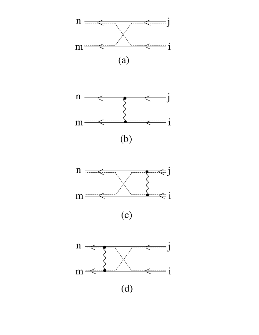
Figure 1: (a): Pauli – or exchange – parameter $\lambda\left({}^{n\ \,j}_{m\ i}\right)$ between two “in” excitons $(i,j)$ giving rise to two “out” excitons $(m,n)$, as defined in eq. (1.4). (b): Direct Coulomb scattering $\xi^{\mathrm{dir}}\left({}^{n\ \,j}_{m\ i}\right)$ as defined in eq. (1.9). (c) and (d): Coulomb exchange scatterings $\xi^{\mathrm{in}}\left({}^{n\ \,j}_{m\ i}\right)$ and $\xi^{\mathrm{out}}\left({}^{n\ \,j}_{m\ i}\right)$ as defined in eqs. (1.10) and (1.11). In $\xi^{\mathrm{in}}$, the Coulomb processes take place between the “in” excitons, while in $\xi^{\mathrm{out}}$, they take place between the “out” excitons. In all these diagrams, the solid lines represent the electrons while the dashed lines represent the holes, the wavy lines representing the Coulomb interactions between the fermions of the excitons represented by double electron-hole lines.

where the $i$ exciton wave function in real space is $\phi_{i}(\mathbf{r}_{e},\mathbf{r}_{h})=\langle\mathbf{r}_{e},\mathbf{r}_{h}|i\rangle\linebreak=\langle\alpha_{e}\mathbf{r}_{e}+\alpha_{h}\mathbf{r}_{h}|\mathbf{Q}_{i}\rangle\,\langle\mathbf{r}_{e}-\mathbf{r}_{h}|\nu_{i}\rangle$, with $\langle\mathbf{R}|\mathbf{Q}\rangle=e^{i\mathbf{Q}.\mathbf{R}}/L^{D/2}$, for sample size $L$ and space dimension $D$. The Pauli parameter $\lambda\left({}^{n\ j}_{m\ i}\right)$ corresponds to a hole exchange when forming the “out” excitons $(m,n)$ from the “in” excitons $(i,j)$ (see Fig.1a). These exchange parameters are not exactly exchange scatterings in the sense that they are dimensionless.

One important property of the $\lambda\left({}^{n\ j}_{m\ i}\right)$ parameters is the fact that if we cross the holes of two excitons twice, we come back to the original situation. As shown in appendix A, we indeed have

$$\sum_{mn}\lambda\left({}^{q\ n}_{p\ m}\right)\,\lambda\left({}^{n\ j}_{m\ i}\right)=\delta_{pi}\,\delta_{qj}\ .$$ (1.5)

Another transparent link between $\lambda\left({}^{n\ j}_{m\ i}\right)$ and the possibility to exchange the carriers in forming two excitons is the fact that we can rewrite any $B_{i}^{\dagger}B_{j}^{\dagger}$ in terms of all the other $B_{m}^{\dagger}B_{n}^{\dagger}$’s according to

$$B_{i}^{\dagger}B_{j}^{\dagger}=-\sum_{mn}\lambda\left({}^{n\ j}_{m\ i}\right)\,B_{m}^{\dagger}B_{n}^{\dagger}\ .$$ (1.6)

As shown in appendix A, this equation is obtained by writing the $i$ exciton in terms of $a_{\mathbf{k}_{e_{i}}}^{\dagger}b_{\mathbf{k}_{h_{i}}}^{\dagger}$ and by forming the $m$ exciton out of $a_{\mathbf{k}_{e_{i}}}^{\dagger}b_{\mathbf{k}_{h_{j}}}^{\dagger}$.

We expect the physics associated to the non-purely bosonic nature of the excitons to appear through exchange processes of various kinds, which are all going to be expressed in terms of these $\lambda\left({}^{n\ j}_{m\ i}\right)$’s. The pure-bosonic exciton approximation used in the effective bosonic Hamiltonian corresponds to take all these $\lambda\left({}^{n\ j}_{m\ i}\right)$’s equal to zero, after having somehow cooked them with Coulomb processes, once and for all, to produce an exciton-exciton scattering “dressed by exchange”.

In addition to non-bosonic behavior, the fact that the excitons are made of indistinguishable carriers makes the Coulomb interaction between excitons quite tricky to define properly, as discussed above. We however need to identify such a quantity in a formal way, if we want to set up a procedure for handling many-body effects between excitons, since of course they are going to contain a certain amount of Coulomb processes. By writing [18,19]

$$\left[H,B_{i}^{\dagger}\right]=E_{i}\ B_{i}^{\dagger}+V_{i}^{\dagger}\ ,$$ (1.7)

$$\left[V_{i}^{\dagger},B_{j}^{\dagger}\right]=\sum_{mn}\xi^{\mathrm{dir}}\left({}^{n\ j}_{m\ i}\right)\,B_{m}^{\dagger}B_{n}^{\dagger}\ ,$$ (1.8)

we in fact generate the set of Coulomb scatterings we want. Indeed, as rederived in appendix B, $\xi^{\mathrm{dir}}\left({}^{n\ j}_{m\ i}\right)$ reads as

$$\xi^{\mathrm{dir}}\left({}^{n\ j}_{m\ i}\right)=\int d\mathbf{r}_{e}\ d\mathbf{r}_{e^{\prime}}\,d\mathbf{r}_{h}\,d\mathbf{r}_{h^{\prime}}\,\phi_{m}^{\ast}(\mathbf{r}_{e},\mathbf{r}_{h})\,\phi_{n}^{\ast}(\mathbf{r}_{e^{\prime}},\mathbf{r}_{h^{\prime}})\left[V_{ee^{\prime}}+V_{hh^{\prime}}-V_{eh^{\prime}}-V_{he^{\prime}}\right]$$

$$\times\phi_{i}(\mathbf{r}_{e},\mathbf{r}_{h})\,\phi_{j}(\mathbf{r}_{e^{\prime}},\mathbf{r}_{h^{\prime}})$$

$$=\xi^{\mathrm{dir}}\left({}^{m\ i}_{n\ j}\right)=\xi^{\mathrm{dir}}\left({}^{j\ n}_{i\ m}\right)^{\ast}\ ,\hskip 207.7052pt$$ (1.9)

with $V_{cd^{\prime}}=e^{2}/|\mathbf{r}_{c}-\mathbf{r}_{d^{\prime}}|$. We see that, in this $\xi^{\mathrm{dir}}\left({}^{n\ j}_{m\ i}\right)$, the “in” exciton $i$ and “out” exciton $m$ are made with the same pairs $(e,h)$ and similarly for the excitons $(j,n)$ ; so that, in $\xi^{\mathrm{dir}}\left({}^{n\ j}_{m\ i}\right)$, the electron-hole Coulomb interaction $(V_{eh^{\prime}}+V_{e^{\prime}h})$ is unambiguously a Coulomb interaction between both the “in” excitons $(i,j)$ and the “out” excitons $(m,n)$ (see Fig.1b). Let us add that, while the exchange parameters $\lambda\left({}^{n\ j}_{m\ i}\right)$ are dimensionless, these $\xi^{\mathrm{dir}}\left({}^{n\ j}_{m\ i}\right)$’s are energy-like quantities.

Using these $\xi^{\mathrm{dir}}\left({}^{n\ j}_{m\ i}\right)$’s and $\lambda\left({}^{n\ j}_{m\ i}\right)$’s, it is possible to derive the many-body physics of excitons in an exact way. In particular, we can construct the two exchange Coulomb scatterings which exist between two excitons. As rederived in appendix C, the one in which the Coulomb interaction takes place between the “in” excitons $(i,j)$ only reads

$$\xi^{\mathrm{in}}\left({}^{n\ j}_{m\ i}\right) = \sum_{rs}\lambda\left({}^{n\ s}_{m\ r}\right)\,\xi^{\mathrm{dir}}\left({}^{s\ j}_{r\ i}\right)$$ (1.10)

$$= \int d\mathbf{r}_{e}\ d\mathbf{r}_{e^{\prime}}\,d\mathbf{r}_{h}\,d\mathbf{r}_{h^{\prime}}\,\phi_{m}^{\ast}(\mathbf{r}_{e},\mathbf{r}_{h^{\prime}})\,\phi_{n}^{\ast}(\mathbf{r}_{e^{\prime}},\mathbf{r}_{h})$$

$$\times \left[V_{ee^{\prime}}+V_{hh^{\prime}}-V_{eh^{\prime}}-V_{he^{\prime}}\right]\phi_{i}(\mathbf{r}_{e},\mathbf{r}_{h})\,\phi_{j}(\mathbf{r}_{e^{\prime}},\mathbf{r}_{h^{\prime}})$$

$$= \xi^{\mathrm{in}}\left({}^{m\ i}_{n\ j}\right)\ .$$

In this Coulomb scattering, the electron-hole part $(V_{eh^{\prime}}+V_{e^{\prime}h})$ is between the “in” excitons $(i,j)$ but “inside” the “out” excitons $(m,n)$ (see Fig.1c). In a similar way,

$$\xi^{\mathrm{out}}\left({}^{n\ j}_{m\ i}\right) = \sum_{rs}\xi^{\mathrm{dir}}\left({}^{n\ s}_{m\ r}\right)\,\lambda\left({}^{s\ j}_{r\ i}\right)$$ (1.11)

$$= \int d\mathbf{r}_{e}\ d\mathbf{r}_{e^{\prime}}\,d\mathbf{r}_{h}\,d\mathbf{r}_{h^{\prime}}\,\phi_{m}^{\ast}(\mathbf{r}_{e},\mathbf{r}_{h})\,\phi_{n}^{\ast}(\mathbf{r}_{e^{\prime}},\mathbf{r}_{h^{\prime}})$$

$$\times \left[V_{ee^{\prime}}+V_{hh^{\prime}}-V_{eh^{\prime}}-V_{he^{\prime}}\right]\phi_{i}(\mathbf{r}_{e},\mathbf{r}_{h^{\prime}})\,\phi_{j}(\mathbf{r}_{e^{\prime}},\mathbf{r}_{h})$$

$$= \xi^{\mathrm{out}}\left({}^{m\ i}_{n\ j}\right)=\left[\xi^{\mathrm{in}}\left({}^{j\ n}_{i\ m}\right)\right]^{\ast}\ ,$$

contains all Coulomb interactions between the “out” excitons $(m,n)$, its electron-hole part being inside the “in” excitons $(i,j)$ (see Fig.1d).

The exchange parameters $\lambda\left({}^{n\ j}_{m\ i}\right)$ being dimensionless, it is possible to build energy-like scatterings out of them, through

$$\mathcal{E}\left({}^{n\ j}_{m\ i}\right)=(E_{m}+E_{n}-E_{i}-E_{j})\,\lambda\left({}^{n\ j}_{m\ i}\right)\ .$$ (1.12)

Note that, as the exciton energy contains the band gap, scatterings having the sum of the “in” and “out” energies, instead of the difference, would depend on the band gap, which is physically unacceptable for many-body effects coming from carrier interactions. Actually, such scatterings never appear. It turns out that $\mathcal{E}\left({}^{n\ j}_{m\ i}\right)$ defined in eq. (1.12) is not an independent scattering but reads in terms of the two exchange Coulomb scatterings defined in eqs. (1.10-11) as (see appendix D)

$$\mathcal{E}\left({}^{n\ j}_{m\ i}\right)=\xi^{\mathrm{in}}\left({}^{n\ j}_{m\ i}\right)-\xi^{\mathrm{out}}\left({}^{n\ j}_{m\ i}\right)\ .$$ (1.13)

From the above discussion, we see that four scatterings between two excitons are energy-like quantities, namely $\xi^{\mathrm{dir}}\left({}^{n\ j}_{m\ i}\right)$, $\xi^{\mathrm{in}}\left({}^{n\ j}_{m\ i}\right)$, $\xi^{\mathrm{out}}\left({}^{n\ j}_{m\ i}\right)$ and $\mathcal{E}\left({}^{n\ j}_{m\ i}\right)$. It is reasonable to expect the exciton-exciton transition rates to read in terms of a linear combination of these four scatterings. The purpose of the present work is to determine this linear combination by using a full-proof procedure.

In order to do it, the first difficulty is to identify the proper way to determine these transition rates. If an exciton-exciton potential were to exist, the exciton-exciton transition rate would result from the Fermi golden rule written in terms of this potential. As such a potential does not exist, it is necessary to construct a formal equivalent of this Fermi golden rule in which $H$ only enters, i. e., in which $H$ is not split as $H_{0}+V$. This formal equivalent, already given in ref. [5], is rederived in the section 2 of this paper, somewhat in details, for completeness.

In order to calculate these transition rates, we also need to identify the relevant “in” and “out” states of the transition. For that, we first note that an $N$-electron-hole-pair state can always be written in terms of free pair states, $a_{\mathbf{k}_{e_{1}}}^{\dagger}b_{\mathbf{k}_{h_{1}}}^{\dagger}\cdots a_{\mathbf{k}_{e_{N}}}^{\dagger}b_{\mathbf{k}_{h_{N}}}^{\dagger}|v\rangle$, the representation on this free pair basis being unique. However, as electron-hole pairs are highly correlated into excitons when their density in Bohr radius unit is small compared to 1, the representation of physical relevance for $N$-pair states in the low density limit, is for sure not the one in terms of free pair states but the one in terms of exciton states, namely $B_{i_{1}}^{\dagger}\cdots B_{i_{N}}^{\dagger}|v\rangle$. This physically relevant representation however is mathematically unpleasant because, due to eq. (1.6), it is not unique, the $N$-exciton basis being overcomplete. As shown in details below, it is actually possible to deal with this unpleasant feature and to calculate the time evolution of any of these $N$-exciton states, using the expression of the Fermi golden rule given in section 2.

Among these $N$-exciton states, the state $(B_{0}^{\dagger})^{N}|v\rangle$, with all the excitons in the same state 0, is particularly simple and of possible physical interest. Indeed, while it is not the exact ground state of $N$ excitons — otherwise it would not evolve with time, — it is close to it. Moreover, this state is the one coupled to $N$ photons tuned to the ground state exciton, so that it plays an important role in all semiconductor optical nonlinear effects.

Although the state $(B_{0}^{\dagger})^{N}|v\rangle$ may appear as particularly simple, let us stress that the precise calculation of its time evolution already contains three major difficulties : (i) The first one is to correctly determine the time evolution of composite bosons taking into account all the carrier exchanges which can take place between them. (ii) The second one comes from the difficulty of handling many-body effects between a large number of these composite particles. (iii) The third one comes from the fact that excitons have a spin degree of freedom. As the exchange processes mix the electrons and holes of two excitons, they also mix their spins. They, in particular, transform two bright excitons with opposite spins, $(\pm 1)$, into two dark excitons with opposite spins $(\pm 2)$. If we take into account these spin degrees of freedom, the exchange parameter $\lambda\left({}^{n\ j}_{m\ i}\right)$, defined through eq. (1.2), becomes a $8^{2}\times 8^{2}$ matrix, each bulk exciton having $2\times 4$ spin degrees of freedom. The situation is somewhat better for narrow quantum wells since the light hole band with spins $(\pm 1/2)$ is well separated from the heavy hole band with spins $(\pm 3/2)$, so that we can forget it. However, the $\lambda\left({}^{n\ j}_{m\ i}\right)$ parameter is still a 16$\times$16 matrix.

In order to reach a deep understanding of the tricky physics involved in these exciton scatterings, we find appropriate to divide this work into three parts.

The present paper I mainly deals with the composite character of the excitons by considering the time evolution of two excitons without spin degree of freedom. This physically corresponds to have two electrons with same spin and two holes with same spin, as possibly produced by the absorption of two circularly polarized photons in a quantum well.

In section 3, we calculate its time evolution using the formalism of the effective bosonic Hamiltonian, as many physicists commonly think about excitons in this way.

In section 4, we calculate the time evolution of the state $(B_{0}^{\dagger})^{2}|v\rangle$ made of two identical composite excitons. From it, we derive the lifetime of this state as well as the transition rate towards another two-exciton state $B_{i}^{\dagger}B_{j}^{\dagger}|v\rangle$, using the formal equivalent of the Fermi golden rule rederived in the section 2 of this paper.

In section 5, we qualitatively discuss the various results obtained by using the effective Hamiltonian in which the excitons are replaced by elementary bosons, with similar quantities obtained for composite excitons.

In section 6, we quantitatively calculate the various elementary scatterings that our composite exciton formalism introduces, namely $\xi^{\mathrm{dir}}$, $\xi^{\mathrm{in}}$, $\xi^{\mathrm{out}}$ and $\mathcal{E}$, in the case of 2D ground state excitons, when the two “in” excitons have the same momentum. We also calculate the transition rate of this two-composite-exciton state, as a function of momentum transfer $Q$, and we compare it to its value when excitons are replaced by elementary bosons. We see that the discrepancy is quite large, except for very small momentum transfer or in the limit of infinitely heavy holes. This strongly questions the impressive fits of experimental results obtained by using the standard exciton-exciton scatterings dressed by exchange, since in real experiments, the hole mass is never that large, to make all exchange scatterings equal. We also see that the exciton-exciton transition rate does not monotically decrease with increasing momentum transfer, but cancels for a finite value of the momentum transfer $Q$. This cancellation may suggest that, in order to get a physically relevant transition rate at large momentum transfer, it might be necessary to go beyond the Fermi golden rule, i. e., the Born approximation. However, it might also be possible that this cancellation survives beyond Born approximation.

The discrepancy between the results obtained for elementary and composite bosons is not fortuitous but has a quite deep origin. Indeed, the bosonic approach has to fail in an irretrievable way because of a mathematical reason. Bosonic exciton states form an orthogonal basis for two-pair states. On the opposite, composite exciton states form an overcomplete set, due to the composite nature of the particles. This overcompleteness is directly linked to the appearance of an additional factor 1/2 between the inverse lifetime and the sum of transition rates, which comes from the difference which exists in the closure relations of composite and elementary bosons, as explicitly shown in ref. [20]. The existence of this factor 1/2 in fact shows that it is impossible to build a set of effective scatterings which would produce both, the lifetime and the transition rate towards another exciton state, correctly. This actually constitutes a strong mathematical proof that we cannot forget the composite nature of the particles, even in the extremely low density limit of just two excitons.

Since the calculations with composite excitons we present here, use quantities we have introduced in various previous works dealing with what we first called “commutation technique”, we have found useful to rederive the important relations between these quantities in a self-contained appendix with coherent notations, some of these derivations being actually simpler than the ones we first gave.

In paper II, we will still consider two excitons only, but we will take into account the spin degrees of freedom of these excitons. From the interplay between direct and exchange scatterings, it is possible to deduce a set of interesting polarization effects between the photons which create the initial state and the bright and dark states produced by its time evolution. In this paper II, we will consider all possible polarizations for quantum wells only. In the case of bulk samples, it is more appropriate to speak in terms of polaritons, instead of excitons. The physics of interacting polaritons is a priori very similar to the one of interacting excitons, the additional photon part of the polariton of course being an elementary boson. We are soon going to propose a new approach to interacting polaritons. This will allow us to derive the various subtle polarization effects which come from the fact that exchange processes between the exciton parts of the polaritons are described by exchange parameters $\lambda\left({}^{n\ j}_{m\ i}\right)$ which now are 64$\times$64 matrices.

Paper III will deal with $N$-exciton states. The change from 2 to $N$ is not small; it induces some very substantial difficulties. One important — but quite tricky — aspect of the $N$-exciton physics is the fact that, unlike for $N$ electrons, many-body effects with $N$ excitons coming from exciton-exciton interaction are not associated to an order in Coulomb interaction, but to an order in the dimensionless parameter associated to density, namely,

$$\eta=N(a_{X}/L)^{D},$$

with $a_{X}$ being the exciton Bohr radius, $L$ the sample size and $D$ the space dimension. The factor $N$ entering this $\eta$ parameter can appear in calculations dealing with $N$ excitons in very many different ways. A careful counting of these $N$’s — and the exact cancellation of overextensive terms in $N^{p}(a_{X}/L)^{qD}$ with $p>q$ — turns out to be rather tricky. However, this is only in this last paper on the time evolution of $N$-exciton states that we will really face the many-body physics of composite excitons in its full complexity. A short report on the scatterings between $N$ excitons, without spin degree of freedom, has been published in ref. [5]. Its key result is the fact that the additional factor $1/2$ between the inverse lifetime and the sum of transition rates here shown for two excitons also exists for $N$ excitons. In a more recent work [20], we have established the link between this additional $1/2$ factor and the overcompleteness of the basis made with composite exciton states, by showing, in details, how this factor $1/2$ appears for $N=2$ and $N=3$ excitons, using the difference which exists in the closure relations of elementary and composite exciton states.

The precise comparison between composite excitons and pure-bosonic excitons done in the present paper, leads us to think that the present “coboson” formalism must be of interest, not only for interacting excitons, but also for many other composite bosons : This coboson formalism, free from bosonization, might reveal unexpected physical effects or, at least, lead to a deeper understanding of the presently known physics. A first idea is to reinvestigate interacting hydrogen atoms, or to reconsider the physics of “ultracold atoms”, which is a domain of very high current interest. We can also think of using it in the on-going extensive studies of interactions between positronium atoms [21] : These atoms seem to be very good candidates to reveal the importance of fermion exchanges as they are formed with fermions having equal masses.

An easy switch from excitons to general cobosons is made by noting that the many-body physics of any other coboson is expected to depend on exchange parameters $\lambda\left({}^{n\ j}_{m\ i}\right)$ and direct scatterings $\xi^{\mathrm{dir}}\left({}^{n\ j}_{m\ i}\right)$, very similar to the ones defined in eqs. (1.4) and (1.9), where $(\mathbf{r}_{e},\mathbf{r}_{h})$ represent the spatial coordinates of the fermion pair at hand, $\phi_{i}(\mathbf{r}_{e},\mathbf{r}_{h})$ being the wave function of the one-pair eigenstate of the system Hamiltonian and $V_{ee^{\prime}}$, $V_{hh^{\prime}}$, $V_{eh}$ the potentials between identical and different fermions.

With respect to the possible representation of the coboson many-body physics, we can note that the many-body theories at hand up to now [15,16] were designed to deal with interacting elementary particles, fermions or bosons ; so that the Feynman diagrams which visualize the underlying perturbative theory, are rather easy to draw, due to the well defined interaction potentials which exist between these elementary quantum particles. For cobosons, we have had to construct, not only a new many-body theory, but also a fully new diagrammatic representation [22]. We have called these new diagrams “Shiva diagrams”, in reference to the multiarm hindu god Shiva, as they have a multiarm structure. These diagrams make appearing the elementary scatterings between two cobosons $\xi^{\mathrm{dir}}\left({}^{n\ j}_{m\ i}\right)$ and $\lambda\left({}^{n\ j}_{m\ i}\right)$. It is of importance to stress that, since an interaction potential between cobosons does not exist, the corresponding diagrams are not a simple visualization of a perturbative theory.

2 The Fermi golden rule in terms of H only

Let us consider that, at initial time $t=0$, the system is in a normalized initial state $|\psi_{0}\rangle$ which is not eigenstate of the system Hamiltonian $H$, otherwise it would not evolve with time. At time $t>0$, this state reads

$$|\psi_{t}\rangle=e^{-i\hat{H}t}|\psi_{0}\rangle\equiv|\psi_{0}\rangle+|\tilde{\psi}_{t}\rangle\ .$$ (2.1)

By definition, $|\tilde{\psi}_{t}\rangle$ is the state change due to the time evolution, while $\hat{H}=H-\langle H\rangle_{0}$, with $\langle H\rangle_{0}=\langle\psi_{0}|H|\psi_{0}\rangle$ being the expectation value of the Hamiltonian in the initial state (we take $\hbar=1$ throughout the paper) : By writing $\hat{H}$ instead of $H$ in eq. (2.1), we have in $|\psi_{t}\rangle$ introduced an irrelevant constant phase factor $e^{i\langle H\rangle_{0}t}$ for convenience.

We then note that

$$\hat{H}|\psi_{0}\rangle\equiv P_{\perp}H|\psi_{0}\rangle\ ,$$ (2.2)

where $P_{\perp}=1-|\psi_{0}\rangle\langle\psi_{0}|$ is the projector over the subspace perpendicular to $|\psi_{0}\rangle$, i.e., $P_{\perp}|\psi_{0}\rangle=0$. It is then easy to check that the state change $|\tilde{\psi}_{t}\rangle$, which physically comes from scatterings in the initial state, can be rewritten as

$$|\tilde{\psi}_{t}\rangle=(e^{-i\hat{H}t}-1)|\psi_{0}\rangle=F_{t}(\hat{H})\,P_{\perp}\,H\,|\psi_{0}\rangle\ ,$$ (2.3)

where we have set

$$F_{t}(E) = \frac{e^{-iEt}-1}{E}=-2i\pi\,e^{-iEt/2}\,\delta_{t}(E)$$

$$\delta_{t}(E) = \frac{\sin(Et/2)}{\pi E}\ ,$$ (2.4)

$\delta_{t}(E)$ being a peaked function of width $2/t$, which reduces to the usual Dirac $\delta$ function in the limit of infinitely large time $t$.

From the definition of the lifetime $\tau_{0}$ of the $|\psi_{0}\rangle$ state, namely, $|\langle\psi_{0}|\psi_{t}\rangle|^{2}=e^{-t/\tau_{0}}$, we have, since $\langle\psi_{t}|\psi_{t}\rangle$ stays equal to 1,

$$\frac{t}{\tau_{0}} \simeq 1-|\langle\psi_{0}|\psi_{t}\rangle|^{2}$$ (2.5)

$$= \langle\psi_{t}|\psi_{t}\rangle-|\langle\psi_{0}|\psi_{t}\rangle|^{2}=\langle\psi_{t}|P_{\perp}|\psi_{t}\rangle\ .$$

By using the state change $|\tilde{\psi}_{t}\rangle$ introduced in eq. (2.1), and the fact that $P_{\perp}|\psi_{t}\rangle=P_{\perp}|\tilde{\psi}_{t}\rangle$, eq. (2.5) can be rewritten as

$$\frac{t}{\tau_{0}}=\langle\tilde{\psi}_{t}|\tilde{\psi}_{t}\rangle-|\langle\psi_{0}|\tilde{\psi}_{t}\rangle|^{2}\ .$$ (2.6)

It is straightforward to check that the above eqs. (2.3) and (2.6) give the well known result in the usual case, i. e., when $H=H_{0}+V$, with $|\psi_{0}\rangle\equiv|0\rangle$ and $H_{0}|n\rangle=\mathcal{E}_{n}|n\rangle$. Indeed, the state change at first order in $V$ is obtained by replacing, in eq. (2.3), $F_{t}(\hat{H})$ by $F_{t}(\hat{H}_{0})$, with $\hat{H}_{0}=H_{0}-\mathcal{E}_{0}$, while $P_{\perp}H|0\rangle=\sum_{n\neq 0}V_{n0}|n\rangle$, so that

$$|\tilde{\psi}_{t}\rangle = F_{t}(\hat{H}_{0})\sum_{n\neq 0}V_{n0}\,|n\rangle+0(V^{2})$$ (2.7)

$$= \sum_{n\neq 0}V_{n0}\,F_{t}(\mathcal{E}_{n}-\mathcal{E}_{0})\,|n\rangle+0(V^{2})\ .$$

The transition rate from $|0\rangle$ to $|n\neq 0\rangle$ follows from

$$\frac{t}{T_{n}}=|\langle n|\psi_{t}\rangle|^{2}=|\langle n|\tilde{\psi}_{t}\rangle|^{2}\simeq 2\pi\,t|V_{n0}|^{2}\,\delta_{t}(\mathcal{E}_{n}-\mathcal{E}_{0})\ ,$$ (2.8)

since we do have

$$|F_{t}(E)|^{2}\simeq|F_{t}(0)F_{t}(E)|\simeq|F_{t}(E)|t=2\pi\,t\,\delta_{t}(E)\ .$$ (2.9)

If we now turn to the lifetime of the $|0\rangle$ state, we find from eq. (2.7) that $\langle 0|\tilde{\psi}_{t}\rangle=0(V^{2})$, so that $t/\tau_{0}$ to second order in $V$ reduces to $\langle\tilde{\psi}_{t}|\tilde{\psi}_{t}\rangle$. Using eq. (2.7) and eq. (2.9), we thus recover the well known result,

$$\frac{1}{\tau_{0}}\simeq 2\pi\,\sum_{n\neq 0}|V_{n0}|^{2}\,\delta_{t}(\mathcal{E}_{n}-\mathcal{E}_{0})\ .$$ (2.10)

We can also get this equation by noting that, as the $|n\rangle$ states are eigenstates of $H_{0}$, they form an orthonormal basis, so that

$$1=\langle\psi_{t}|\psi_{t}\rangle=\langle\psi_{t}|\sum_{n}|n\rangle\langle n||\psi_{t}\rangle=|\langle 0|\psi_{t}\rangle|^{2}+\sum_{n\neq 0}|\langle n|\psi_{t}\rangle|^{2}\ .$$ (2.11)

Consequently, due to eq. (2.5) we must have

$$\frac{1}{\tau_{0}}\simeq\sum_{n\neq 0}\frac{1}{T_{n}}\ ,$$ (2.12)

in agreement with eqs. (2.8,10).

3 Two bosonic excitons

Let us first follow a procedure, quite often found in the literature, which assumes that composite excitons can be validly replaced by elementary bosonic excitons in the low density limit. Their creation operators are then such that

$$\left[\overline{B}_{i},\overline{B}_{j}^{\dagger}\right]=\delta_{ij}\ ,$$ (3.1)

provided that the composite character of the excitons is included in the Hamiltonian through the matrix elements of an appropriate phenomenological exciton-exciton interaction. The semiconductor Hamiltonian is then replaced by an effective bosonic Hamiltonian $H_{\mathrm{eff}}=H_{\mathrm{x}}+V_{\mathrm{xx}}$, where the one-body part reads

$$H_{\mathrm{x}}=\sum_{i}E_{i}\,\overline{B}_{i}^{\dagger}\,\overline{B}_{i}\ ,$$ (3.2)

while the exciton-exciton potential is written as

$$V_{\mathrm{xx}}=\frac{1}{2}\sum_{mnij}V_{mnij}\,\overline{B}_{m}^{\dagger}\,\overline{B}_{n}^{\dagger}\,\overline{B}_{i}\,\overline{B}_{j}\ ,$$ (3.3)

with $V_{mnij}=V_{nmij}=V_{mnji}$ due to possible changes in the bold indices, while $V_{mnij}=V_{ijmn}^{\ast}$ in order to insure hermiticity, $H_{\mathrm{eff}}=H_{\mathrm{eff}}^{\dagger}$.

As, for Hamiltonian eigenstates, $\delta_{mi}=\langle m|i\rangle=\langle v|\overline{B}_{m}\overline{B}_{i}^{\dagger}|v\rangle$, we have in the two-exciton subspace, due to eq. (3.1),

$$\langle v|\overline{B}_{m}\,\overline{B}_{n}\,\overline{B}_{i}^{\dagger}\,\overline{B}_{j}^{\dagger}|v\rangle=\langle v|\overline{B}_{m}\,(\overline{B}_{i}^{\dagger}\,\overline{B}_{n}+\delta_{in})\,\overline{B}_{j}^{\dagger}|v\rangle=\delta_{mi}\,\delta_{nj}+\delta_{mj}\,\delta_{ni}\ .$$ (3.4)

Consequently, the normalized two-exciton states are given by

$$|\overline{\phi}_{ij}\rangle=\frac{\overline{B}_{i}^{\dagger}\,\overline{B}_{j}^{\dagger}|v\rangle}{\sqrt{1+\delta_{ij}}}=|\overline{\phi}_{ji}\rangle\ .$$ (3.5)

Transition rates towards other two-exciton states exist because $|\overline{\phi}_{ij}\rangle$ is not eigenstate of the Hamiltonian, so that this state evolves with time. In this time evolution, the $|\overline{\phi}_{ij}\rangle$ state gets non-zero projections over $|\overline{\phi}_{mn}\rangle$ with $(mn)\neq(ij)$. For simplicity, let us study the scattering of two excitons in the same state $0\,{\bf\equiv}\,(\nu_{0},\mathbf{Q}_{0})$, towards any other two-exciton state. The normalized initial state is then $|\overline{\psi}_{t=0}\rangle=|\overline{\phi}_{00}\rangle=(1/\sqrt{2})\overline{B}_{0}^{{\dagger}2}|v\rangle$. By noting that, due to eqs. (3.2, 3.3),

$$H_{\mathrm{eff}}\,\overline{B}_{p}^{\dagger}\overline{B}_{q}^{\dagger}|v\rangle=(E_{p}+E_{q})\,\overline{B}_{p}^{\dagger}\overline{B}_{q}^{\dagger}|v\rangle+\sum_{mn}V_{mnpq}\,\overline{B}_{m}^{\dagger}\,\overline{B}_{n}^{\dagger}|v\rangle\ ,$$ (3.6)

we get, from eq. (3.4), the expectation value of the Hamiltonian in this $|\overline{\psi}_{0}\rangle$ initial state as

$$\langle H_{\mathrm{eff}}\rangle_{0}=\langle\overline{\phi}_{00}|H_{\mathrm{eff}}|\overline{\phi}_{00}\rangle=2\,E_{0}+V_{0000}$$ (3.7)

Using eqs. (2.2, 3.6, 3.7), we then find

$$P_{\perp}\,H_{\mathrm{eff}}\,\overline{B}_{0}^{{\dagger}2}|v\rangle=(H_{\mathrm{eff}}-\langle H_{\mathrm{eff}}\rangle_{0})\overline{B}_{0}^{{\dagger}2}|v\rangle=(V_{\mathrm{xx}}-V_{0000})\overline{B}_{0}^{{\dagger}2}|v\rangle=\sum_{mn\neq 00}V_{mn00}\overline{B}_{m}^{\dagger}\overline{B}_{n}^{\dagger}|v\rangle\ ,$$ (3.8)

since, due to eqs. (3.3,3.4) we do have

$$V_{\mathrm{xx}}\,\overline{B}_{0}^{{\dagger}2}|v\rangle=\frac{1}{2}\sum_{mnij}V_{mnij}\overline{B}_{m}^{\dagger}\overline{B}_{n}^{\dagger}|v\rangle\langle v|\overline{B}_{i}\overline{B}_{j}\overline{B}_{0}^{{\dagger}2}|v\rangle=\sum_{mn}V_{mn00}\overline{B}_{m}^{\dagger}\overline{B}_{n}^{\dagger}|v\rangle\ .$$ (3.9)

To first order in the interactions, the state change $|\tilde{\overline{\psi}}_{t}\rangle$, given by eq. (2.3), is obtained by replacing $\hat{H}$ by its zero order contribution, namely $H_{\mathrm{x}}-2E_{0}$. This leads to

$$|\tilde{\overline{\psi}}_{t}\rangle=\sum_{mn\neq 00}F_{t}(E_{m}+E_{n}-2E_{0})V_{mn00}\frac{\overline{B}_{m}^{\dagger}\overline{B}_{n}^{\dagger}|v\rangle}{\sqrt{2}}+O(V^{2})\ .$$ (3.10)

It is clear from the start that, for physically relevant — not too large — momentum ${\bf Q}_{0}$, energy conservation imposes the scattered states $(m,n)$ to belong to the same relative motion subspace $\nu_{0}$ as the initial excitons. We then note that momentum conservation in the Coulomb interactions leading to the exciton-exciton scattering $V_{mn00}$ imposes the $(m,n)$ states forming $|\tilde{\overline{\psi}}_{t}\rangle$ to be such that $m=(\nu_{0},\mathbf{Q}_{0}+\mathbf{q})$ and $n=(\nu_{0},\mathbf{Q}_{0}-\mathbf{q})$, the momentum transfer $\mathbf{q}$ differing from $\mathbf{0}$, in order for $(m,n)$ to differ from $(0,0)$. Consequently, the scattered states are made of different excitons, $m\neq n$.

The transition rate towards a (normalized) two-bosonic-exciton state $|\overline{\phi}_{ij}\rangle$ with $(i,j)\neq(0,0)$ is thus given by

$$\frac{t}{\overline{T}_{ij}}\simeq|\langle\overline{\phi}_{ij}|\overline{\psi}_{t}\rangle|^{2}=|\langle\overline{\phi}_{ij}|\tilde{\overline{\psi}}_{t}\rangle|^{2}\ ,$$ (3.11)

as $\langle\overline{\phi}_{ij}|\overline{\phi}_{00}\rangle=0$ for $(i,j)\neq(0,0)$, due to eq. (3.4). This leads to

$$\frac{t}{\overline{T}_{ij\neq 00}}\simeq\frac{1}{2(1+\delta_{ij})}\left|\sum_{mn\neq 00}F_{t}(E_{m}+E_{n}-2E_{0})\,V_{mn00}\,\langle v|\overline{B}_{i}\overline{B}_{j}\overline{B}_{m}^{\dagger}\overline{B}_{n}^{\dagger}|v\rangle\right|^{2}\ .$$ (3.12)

We then note that, due to energy and momentum conservation, this transition rate differs from zero for $i\neq j$ only. So that eqs. (3.4,2.9) give the transition rate from $|\overline{\phi}_{00}\rangle$ to $|\overline{\phi}_{ij\neq 00}\rangle$ as

$$\frac{1}{\overline{T}_{ij\neq 00}} \simeq 4\,\pi\ |V_{ij00}|^{2}\,\delta_{t}(E_{i}+E_{j}-2E_{0})$$ (3.13)

$$= 2\pi\left|\langle\overline{\phi}_{ij}|V_{\mathrm{xx}}|\overline{\phi}_{00}\rangle\right|^{2}\delta_{t}(E_{i}+E_{j}-2E_{0})\ ,$$

in agreement with the well known expression of the Fermi golden rule.

If we now turn to the bosonic-exciton lifetime, we see from eq. (3.10) that $\langle\overline{\phi}_{00}|\tilde{\overline{\psi}}_{t}\rangle=0(V^{2})$, so that, to second order in $V$, we have

$$\frac{t}{\overline{\tau_{0}}} \simeq \langle\tilde{\overline{\psi}}_{t}|\tilde{\overline{\psi}}_{t}\rangle$$ (3.14)

$$\simeq \frac{1}{2}\sum_{mn\neq 00,ij\neq 00}F_{t}^{\ast}(E_{i}+E_{j}-2E_{0})F_{t}(E_{m}+E_{n}-2E_{0})V_{ij00}^{\ast}V_{mn00}\,\langle v|\overline{B}_{i}\overline{B}_{j}\overline{B}_{m}^{\dagger}\overline{B}_{n}^{\dagger}|v\rangle$$

$$\simeq t\ 2\,\pi\,\sum_{ij\neq 00}|V_{ij00}|^{2}\,\delta_{t}(E_{i}+E_{j}-2E_{0})\ .$$

We thus end with

$$\frac{1}{\overline{\tau}_{0}}\simeq\frac{1}{2}\sum_{ij\neq 00}\frac{1}{\overline{T}_{ij}}=\sum_{\mathrm{couples}(i,j)\neq(0,0)}\frac{1}{\overline{T}_{ij}}\ .$$ (3.15)

We can also recover the above link between lifetime and transition rates by using the closure relation for two-bosonic exciton states. Since any 2-boson state $|\overline{\Phi}\rangle$ can be rewritten as

$$|\overline{\Phi}\rangle=\frac{1}{2!}\sum_{ij}\overline{B}_{i}^{\dagger}\,\overline{B}_{j}^{\dagger}|v\rangle\langle v|\overline{B}_{i}\overline{B}_{j}|\overline{\Phi}\rangle\ ,$$ (3.16)

— easy to check from eq. (3.4), — the closure relation for elementary bosons reads in terms of the normalized bosonic exciton states $|\overline{\phi}_{ij}\rangle$ as

$$I=\frac{1}{2}\sum_{ij}\overline{B}_{i}^{\dagger}\,\overline{B}_{j}^{\dagger}|v\rangle\langle v|\overline{B}_{i}\overline{B}_{j}=\frac{1}{2}\sum_{ij}(1+\delta_{ij})|\overline{\phi}_{ij}\rangle\langle\overline{\phi}_{ij}|=\sum_{i}|\overline{\phi}_{ii}\rangle\langle\overline{\phi}_{ii}|+\frac{1}{2}\sum_{i\neq j}|\overline{\phi}_{ij}\rangle\langle\overline{\phi}_{ij}|\ .$$ (3.17)

If we use this closure relation into $\langle\overline{\psi}_{t}|\overline{\psi}_{t}\rangle$, we get

$$1=\langle\overline{\psi}_{t}|\overline{\psi}_{t}\rangle=\langle\overline{\psi}_{t}|\left[\sum_{i}|\overline{\phi}_{ii}\rangle\langle\overline{\phi}_{ii}|+\frac{1}{2}\sum_{i\neq j}|\overline{\phi}_{ij}\rangle\langle\overline{\phi}_{ij}|\right]|\overline{\psi}_{t}\rangle\ .$$ (3.18)

We now remember that $|\overline{\psi}_{t}\rangle=|\overline{\phi}_{00}\rangle+|\tilde{\overline{\psi}}_{t}\rangle$, where $|\tilde{\overline{\psi}}_{t}\rangle$ contains terms in $mn\neq 00$ with $m\neq n$ due to momentum conservation in the Coulomb scatterings producing the time evolution. This leads to $\langle\overline{\phi}_{ii}|\overline{\psi}_{t}\rangle=0$ for $i\neq 0$, while the sum over $i\neq j$ can be replaced by a sum over $(ij\neq 00)$. So that we end with the lifetime of the $|\overline{\phi}_{00}\rangle$ state given by

$$\frac{t}{\overline{\tau}_{0}}\simeq 1-|\langle\overline{\phi}_{00}|\overline{\psi}_{t}\rangle|^{2}=\frac{1}{2}\sum_{ij\neq 00}|\langle\overline{\phi}_{ij}|\overline{\psi}_{t}\rangle|^{2}\simeq\frac{t}{2}\sum_{ij\neq 00}\frac{1}{\overline{T}_{ij}}\ ,$$ (3.19)

in agreement with eq. (3.15).

4 Two composite excitons

We now turn to real physics with excitons made of electron-hole pairs. The semiconductor Hamiltonian, $H=H_{\mathrm{e}}+H_{\mathrm{h}}+\mathcal{V}_{\mathrm{ee}}+\mathcal{V}_{\mathrm{hh}}+\mathcal{V}_{\mathrm{eh}}$, reads in terms of electron and hole creation operators $a_{\mathbf{k}}^{\dagger}$ and $b_{\mathbf{k}}^{\dagger}$, with any two-pair state a priori written as a sum of products of two free pair operators $a_{\mathbf{k}_{e}}^{\dagger}b_{\mathbf{k}_{h}}^{\dagger}$. As in the low density limit, these pairs form excitons, the representation of two-pair states in terms of two excitons is clearly the relevant one in this limit, the way to go from the free-pair representation to the exciton representation being given by eq. (A5), in appendix A.

Although physically relevant, this exciton representation raises some major difficulties which have to be faced and handled if we want to use it safely. The first one comes from the fact that the $N$-exciton states are not orthogonal for $N=2$ already. Indeed, by using eqs. (1.2, 1.3) and by noting that $D_{ni}|v\rangle=0$, which readily follows from eq. (A.3), we find

$$\langle v|B_{m}B_{n}B_{i}^{\dagger}B_{j}^{\dagger}|v\rangle = \langle v|B_{m}(B_{i}^{\dagger}B_{n}+\delta_{ni}-D_{ni})B_{j}^{\dagger}|v\rangle$$ (4.1)

$$= \delta_{mi}\,\delta_{nj}+\delta_{mj}\,\delta_{ni}-\lambda\left({}^{n\ j}_{m\ i}\right)-\lambda\left({}^{m\ j}_{n\ i}\right)\ ,$$

which differs from the scalar product of two-boson-exciton states given in eq. (3.4) by the presence of the two $\lambda$ terms. Because of these exchange parameters which originate from the composite character of the excitons via the deviation-from-boson operator $D_{mi}$, we see that, unlike boson excitons, the two-exciton states are never orthogonal, even if the excitons $(m,n)$ are different from $(i,j)$.

Another difficulty, which is related to the above one, comes from the fact that there is an infinite number of representations of a given state $|\psi\rangle$ in terms of excitons. This difficulty is directly linked to the identity (1.6). Indeed, if we know one representation of a state $|\psi\rangle$ in terms of excitons, we can produce an infinite number of equally valid representations by using this equation (1.6). Indeed

$$|\psi\rangle = \sum_{ij}\psi_{ij}\,B_{i}^{\dagger}B_{j}^{\dagger}|v\rangle$$ (4.2)

$$= \sum_{mn}\left(-\sum_{ij}\lambda\left({}^{n\ j}_{m\ i}\right)\,\psi_{ij}\right)B_{m}^{\dagger}B_{n}^{\dagger}|v\rangle$$

$$= \sum_{ij}\left(x\,\psi_{ij}-y\,\sum_{mn}\lambda\left({}^{j\ n}_{i\ m}\right)\,\psi_{mn}\right)\,B_{i}^{\dagger}B_{j}^{\dagger}|v\rangle$$

$$= \sum_{ij}\psi_{ij}(x,y)\,B_{i}^{\dagger}B_{J}^{\dagger}|v\rangle\ ,$$

where $x$ and $y$ are two arbitrary constants such that $x+y=1$. Starting from one representation of $|\psi\rangle$ in terms of excitons, we can thus construct an infinite number of prefactors $\psi_{ij}(x,y)$ for the same state $|\psi\rangle$.

In spite of these difficulties, the exciton representation is the relevant one at low density, the system being closer to excitons than to free pairs. Consequently, it is necessary to learn how to work with these exciton states properly and to cope with all the underlying problems associated to them.

In this work, we are interested in the exciton-exciton transition rate. Such a transition rate exists because the two-exciton states are not eigenstates of the semiconductor Hamiltonian, so that they evolve with time. Due to eq. (4.1), these normalized two-exciton states read, instead of eq. (3.5),

$$|\phi_{ij}\rangle=\frac{B_{i}^{\dagger}B_{j}^{\dagger}|v\rangle}{\sqrt{1+\delta_{ij}-\lambda\left({}^{j\ j}_{i\ i}\right)-\lambda\left({}^{i\ j}_{j\ i}\right)}}\ .$$ (4.3)

As for bosonic excitons, let us take as initial state two excitons in the same state $0\,{\bf\equiv}\,(\nu_{0},\mathbf{Q}_{0})$,

$$|\psi_{0}\rangle=|\phi_{00}\rangle=\frac{B_{0}^{{\dagger}2}|v\rangle}{\sqrt{2-2\lambda\left({}^{0\ 0}_{0\ 0}\right)}}\ .$$ (4.4)

In order to calculate its time change $|\tilde{\psi}_{t}\rangle$ given in eq. (2.3), we first need to calculate $H\,B_{0}^{{\dagger}2}|v\rangle$. Using eqs. (1.7, 1.8) and noting that $V_{i}^{\dagger}|v\rangle=0$, which follows from eq. (1.7), we readily find

$$(H-2E_{0})B_{0}^{{\dagger}2}|v\rangle=\sum_{mn}\xi^{\mathrm{dir}}\left({}^{n\ 0}_{m\ 0}\right)\,B_{m}^{\dagger}B_{n}^{\dagger}|v\rangle\ .$$ (4.5)

Before going further, let us mention an additional difficulty with these exciton states, which is another aspect of the one leading to eq. (4.2). Making use of eq. (1.6), one sees that the RHS of the above equation is unchanged if we replace $\xi^{\mathrm{dir}}\left({}^{n\ 0}_{m\ 0}\right)$ by $-\xi^{\mathrm{in}}\left({}^{n\ 0}_{m\ 0}\right)$, since $\xi^{\mathrm{dir}}$ and $\xi^{\mathrm{in}}$ are related by eq. (1.10). This shows, using the same procedure as in eq. (4.2), that we can, in eq. (4.5), replace $\xi^{\mathrm{dir}}\left({}^{n\ 0}_{m\ 0}\right)$ by $\xi\left({}^{n\ 0}_{m\ 0}\right)$, with

$$\xi\left({}^{n\ j}_{m\ i}\right)\equiv a\,\xi^{\mathrm{dir}}\left({}^{n\ j}_{m\ i}\right)-b\,\xi^{\mathrm{in}}\left({}^{n\ j}_{m\ i}\right)\ ,$$ (4.6)

where $a$ and $b$ are two arbitrary constants such that $a+b=1$, with $a$ and $b$ chosen real for simplicity. Consequently, the scattering of two excitons into two other excitons may seem somewhat arbitrary.

We can note that

$$\xi^{\prime}\left({}^{n\ j}_{m\ i}\right)=-\sum_{pq}\lambda\left({}^{n\ q}_{m\ p}\right)\,\xi\left({}^{q\ j}_{p\ i}\right)=-a\xi^{\mathrm{in}}\left({}^{n\ j}_{m\ i}\right)+b\xi^{\mathrm{dir}}\left({}^{n\ j}_{m\ i}\right)\ ,$$ (4.7)

which follows from eq. (1.10) and eq. (C.1) in appendix C. Consequently, the scatterings $\xi\left({}^{n\ j}_{m\ i}\right)$ which stay unchanged by carrier exchanges, i. e., by, in eq. (4.5), rewriting $B_{m}^{\dagger}B_{n}^{\dagger}$ according to eq. (1.6), are such that $\xi\left({}^{n\ j}_{m\ i}\right)=\xi^{\prime}\left({}^{n\ j}_{m\ i}\right)$. They thus correspond to $a=b=1/2$. This may lead to think that, among all the possible exciton-exciton Coulomb scatterings $\xi\left({}^{n\ j}_{m\ i}\right)$, the ones which are physically relevant, due to possible carrier exchanges between composite excitons, are precisely those stable under these exchanges, i. e., those with $a=b=1/2$.

Nevertheless, in order to fully master the apparent arbitrariness in the exciton-exciton Coulomb scatterings, we are, in the following, going to perform all calculations with $\xi$’s having arbitrary $a$ and $b$. This will allow us to see, in details, where this apparent arbitrariness actually disappears from physical quantities. We will also see that the scatterings with $a=b=1/2$, even if they may appear as physically nicer, are not any better than the other ones, with respect to the correctness of the lifetime and transition rates.

Using eq. (4.5), we find that the expectation value of the Hamiltonian in the initial state $|\phi_{00}\rangle$ is given by

$$\langle H\rangle_{0}=\langle\phi_{00}|H|\phi_{00}\rangle=2\,E_{0}+\sum_{mn}\xi\left({}^{n\ 0}_{m\ 0}\right)\,\frac{\langle v|B_{0}^{2}B_{m}^{\dagger}B_{n}^{\dagger}|v\rangle}{2-2\lambda\left({}^{0\ 0}_{0\ 0}\right)}\ .$$ (4.8)

Using eqs. (4.1,4.6,4.7), we first see that the sum in the above equation does not depend on the arbitrariness of $\xi$. Indeed, we do have

$$\sum_{mn}\langle v|B_{p}B_{q}B_{m}^{\dagger}B_{n}^{\dagger}|v\rangle\,\xi\left({}^{n\ j}_{m\ i}\right) = \left[\xi\left({}^{q\ j}_{p\ i}\right)-\sum_{mn}\lambda\left({}^{q\ n}_{p\ m}\right)\,\xi\left({}^{n\ j}_{m\ i}\right)\right]+(p\leftrightarrow q)$$ (4.9)

$$= \left[\xi\left({}^{q\ j}_{p\ i}\right)+\xi^{\prime}\left({}^{q\ j}_{p\ i}\right)\right]+(p\leftrightarrow q)$$

$$= \left[\xi^{\mathrm{dir}}\left({}^{q\ j}_{p\ i}\right)-\xi^{\mathrm{in}}\left({}^{q\ j}_{p\ i}\right)\right]+(p\leftrightarrow q)\ ,$$

whatever $a$ and $b$ are. Consequently, the Hamiltonian expectation value does not depend on the particular scattering $\xi$ used to calculate it, as physically reasonable :

$$\langle H\rangle_{0}=2E_{0}+\frac{\xi^{\mathrm{dir}}\left({}^{0\ 0}_{0\ 0}\right)-\xi^{\mathrm{in}}\left({}^{0\ 0}_{0\ 0}\right)}{1-\lambda\left({}^{0\ 0}_{0\ 0}\right)}\ .$$ (4.10)

In the case of excitons, where the Coulomb repulsion between identical fermions is equal to the attraction of different fermions, the direct scattering is such that $\xi^{\mathrm{dir}}\left({}^{0\ 0}_{0\ 0}\right)=0$, due to eq. (B.18). However, in order for this work to be easily transposed to other cobosons like the cold gases of atomic physics for which the interactions between fermions do not have the above symmetry, we will keep writing this $\xi^{\mathrm{dir}}\left({}^{0\ 0}_{0\ 0}\right)$ in the following equations.

Using the value of $\langle H\rangle_{0}$ given in eq. (4.10), it is easy to see that $P_{\perp}HB_{0}^{{\dagger}2}|v\rangle$ entering the state change $|\tilde{\psi}_{t}\rangle$ reads

$$P_{\perp}\,H\,B_{0}^{{\dagger}2}|v\rangle=(H-\langle H\rangle_{0})B_{0}^{{\dagger}2}|v\rangle=\sum_{mn}\xi\left({}^{n\ 0}_{m\ 0}\right)\,B_{m}^{\dagger}B_{n}^{\dagger}|v\rangle-V_{00}\,B_{0}^{{\dagger}2}|v\rangle\ ,$$ (4.11)

with $V_{00}$ defined as $V_{00}=\left[\xi^{\mathrm{dir}}\left({}^{0\ 0}_{0\ 0}\right)-\xi^{\mathrm{in}}\left({}^{0\ 0}_{0\ 0}\right)\right]/\left[1-\lambda\left({}^{0\ 0}_{0\ 0}\right)\right]$. Equation (4.11) makes $P_{\perp}HB_{0}^{{\dagger}2}|v\rangle$ linear in Coulomb interaction, as physically expected.

If we now consider the transition rate from the initial state $|\phi_{00}\rangle$ to another exciton state $|\phi_{ij\neq 00}\rangle$, a naïve way to define this transition rate would be

$$\frac{t}{T^{\mathrm{na\ddot{\i}ve}}_{ij}}\simeq|\langle\phi_{ij}|\psi_{t}\rangle|^{2}=|\langle\phi_{ij}|\phi_{00}\rangle+\langle\phi_{ij}|\tilde{\psi}_{t}\rangle|^{2}\ .$$ (4.12)

We then note that, while in usual problems dealing with transition rates, the initial and final states are orthogonal, being eigenstates of the unperturbed Hamiltonian $H_{0}$, this is not true for transitions between exciton states. Indeed, due to eq. (4.1), the initial and final states are such that

$$\langle\phi_{ij\neq 00}|\phi_{00}\rangle=-\frac{2\,\lambda\left({}^{j\ 0}_{i\ 0}\right)}{\sqrt{\left[2-2\lambda\left({}^{0\ 0}_{0\ 0}\right)\right]\left[1+\delta_{ij}-\lambda\left({}^{j\ j}_{i\ i}\right)-\lambda\left({}^{i\ j}_{j\ i}\right)\right]}}\neq 0\ .$$ (4.13)

However, since this scalar product does not depend on time, while $|\tilde{\psi}_{t=0}\rangle$ is equal to zero, as seen from eq. (2.3), the RHS of eq. (4.12) does not cancel for $t=0$, so that it cannot be equal to $t/T_{ij}$. Actually, this nonzero contribution to the transition rate is completely unphysical because it corresponds to the fraction of the $|\phi_{ij\neq 00}\rangle$ state already present in the initial state, due to the nonorthogonality of composite exciton states.

When we speak of transition rate, we have in mind a transition induced by the time evolution of the system, the state change associated to this time evolution being nothing but $|\tilde{\psi}_{t}\rangle$. Consequently, the physically relevant expression of the transition rate from $|\phi_{00}\rangle$ to $|\phi_{ij\neq 00}\rangle$ cannot be eq. (4.12), but instead

$$\frac{t}{T_{ij}}=|\langle\phi_{ij}|\tilde{\psi}_{t}\rangle|^{2}=\left|\langle\phi_{ij}|F_{t}(\hat{H})\,P_{\perp}H|\phi_{00}\rangle\right|^{2}\ ,$$ (4.14)

in which we have used eq. (2.3) for $|\tilde{\psi}_{t}\rangle$. Since, due to eq. (4.11), $P_{\perp}H|\phi_{00}\rangle$ is linear in Coulomb interaction, we just have to take $F_{t}(\hat{H})$ at zero order in Coulomb interaction, in order to get the transition rate at second order. However, unlike for bosonic excitons for which a zero order Hamiltonian $H_{\mathrm{x}}$ exists, the zero order in Coulomb interaction is less clear for composite excitons. Of course, we guess that “zero order” means to replace in eq. (4.14) $\hat{H}$ by $(E_{i}+E_{j}-2E_{0})$. Actually, this can be shown in a clean way. By using the following identities, rederived in appendix E,

$$\frac{1}{a-H}\,B_{i}^{\dagger}=\left(B_{i}^{\dagger}+\frac{1}{a-H}\,V_{i}^{\dagger}\right)\,\frac{1}{a-H-E_{i}}\ ,$$ (4.15)

$$e^{-iHt}\,B_{i}^{\dagger}=B_{i}^{\dagger}\,e^{-i(H+E_{i})t}+W_{i}^{\dagger}(t)\ ,$$ (4.16)

with $W_{i}^{\dagger}(t)$ given by

$$W_{i}^{\dagger}(t)=-\int_{-\infty}^{+\infty}\frac{dx}{2i\pi}\,\frac{e^{-ixt}}{x-H+i\eta}\,V_{i}^{\dagger}\,\frac{1}{x-H-E_{i}+i\eta}\ ,$$ (4.17)

it is straightforward to show that

$$F_{t}(H-a)\,B_{i}^{\dagger}=B_{i}^{\dagger}\,F_{t}(H+E_{i}-a)+\mathcal{V}_{i}^{\dagger}(t)\ ,$$ (4.18)

where $\mathcal{V}_{i}^{\dagger}(t)$, equal to

$$\mathcal{V}_{i}^{\dagger}(t)=\left[F_{t}(H-a)\,V_{i}^{\dagger}-e^{iat}\,W_{i}^{\dagger}(t)\right]\,\frac{1}{a-H-E_{i}}\ ,$$ (4.19)

gives zero when acting on vacuum, while, due to eq. (1.8), it gives a state which is at least linear in $\xi$ when acting on excitons. Consequently, since $(H-E_{j})\,B_{j}^{\dagger}|v\rangle=0$, we do end with the result we guessed, namely

$$F_{t}(H-\langle H\rangle_{0})\,B_{i}^{\dagger}B_{j}^{\dagger}|v\rangle = F_{t}(E_{i}+E_{j}-\langle H\rangle_{0})\,B_{i}^{\dagger}B_{j}^{\dagger}|v\rangle+\mathcal{V}_{i}^{\dagger}(t)\,B_{j}^{\dagger}|v\rangle$$ (4.20)

$$= F_{t}(E_{i}+E_{j}-2E_{0})\,B_{i}^{\dagger}B_{j}^{\dagger}|v\rangle+O(\xi)\ .$$

The contribution to the transition rate, quadratic in Coulomb scatterings, is thus given by

$$\frac{t}{T_{ij\neq 00}}=\frac{\left|F_{t}(E_{i}+E_{j}-2E_{0})\,\langle v|B_{i}B_{j}\left\{\sum_{mn}\xi\left({}^{n\ 0}_{m\ 0}\right)\,B_{m}^{\dagger}B_{n}^{\dagger}|v\rangle-V_{00}\,B_{0}^{{\dagger}2}|v\rangle\right\}\right|^{2}}{\left[1+\delta_{ij}-\lambda\left({}^{j\ j}_{i\ i}\right)-\lambda\left({}^{i\ j}_{j\ i}\right)\right]\left[2-2\lambda\left({}^{0\ 0}_{0\ 0}\right)\right]}\ .$$ (4.21)

Due to eq. (4.9), the scalar product with the sum in the above equation gives $2\left[\xi^{\mathrm{dir}}\left({}^{j\ 0}_{i\ 0}\right)-\xi^{\mathrm{in}}\left({}^{j\ 0}_{i\ 0}\right)\right]$ whatever $a$ and $b$ are, while the scalar product of the other term reduces to $\left[-2\lambda\left({}^{j\ 0}_{i\ 0}\right)\right]V_{00}$, for $ij\neq 00$. We then note, either from dimensional arguments or from precise calculations using eq. (1.4), that the exchange parameters between bound state excitons are of the order of $(a_{X}/L)^{D}$. So that this other term, which is a factor $(a_{X}/L)^{D}$ smaller than the sum, can be neglected in eq. (4.21). Since energy and momentum conservation in the transition rate imposes $i\neq j$, we end with a transition rate from $|\phi_{00}\rangle$ to $|\phi_{ij\neq 00}\rangle$ given by

$$\frac{1}{T_{ij\neq 00}}=4\,\pi\left|\xi^{\mathrm{dir}}\left({}^{j\ 0}_{i\ 0}\right)-\xi^{\mathrm{in}}\left({}^{j\ 0}_{i\ 0}\right)\right|^{2}\,\delta_{t}(E_{i}+E_{j}-2E_{0})\ .$$ (4.22)

Note that the above expression is formally identical to the one for bosonic excitons obtained in eq. (3.13). We will come back to this similarity later on.

Let us now turn to the lifetime of the state $|\phi_{00}\rangle$. We can obtain it from eq. (2.6). By replacing $F_{t}(\hat{H})$ by its zero order contribution, we first note, using eq. (2.3) with $F_{t}$ acting on the left, that

$$\langle\phi_{00}|\tilde{\psi}_{t}\rangle\simeq F_{t}(0)\langle\phi_{00}|P_{\perp}H\phi_{00}\rangle$$ (4.23)

is second order in $\xi$ since $\langle\phi_{00}|P_{\perp}=0$. Consequently, $|\langle\phi_{00}|\tilde{\psi}_{t}\rangle|^{2}$ gives a contribution to the lifetime in $\xi^{4}$. If we now turn to $\langle\tilde{\psi}_{t}|\tilde{\psi}_{t}\rangle$, it reads, using eq. (4.11),

$$\langle\tilde{\psi}_{t}|\tilde{\psi}_{t}\rangle=\frac{1}{2-2\lambda\left({}^{0\ 0}_{0\ 0}\right)}\,\langle v|B_{0}^{2}HP_{\perp}\left\{\sum_{mn}|F_{t}(E_{m}+E_{n}-2E_{0})|^{2}\xi\left({}^{n\ 0}_{m\ 0}\right)B_{m}^{\dagger}B_{n}^{\dagger}|v\rangle\right.$$

$$\left.-V_{00}F_{t}(0)B_{0}^{{\dagger}2}|v\rangle\right\}+O(\xi^{3})\ .$$ (4.24)

Since $P_{\perp}B_{0}^{{\dagger}2}|v\rangle=0$, we can drop the $B_{0}^{{\dagger}2}|v\rangle$ terms of the bracket, so that

$$\langle\tilde{\psi}_{t}|\tilde{\psi}_{t}\rangle = \frac{1}{2-2\lambda\left({}^{0\ 0}_{0\ 0}\right)}\,\langle v|B_{0}^{2}HP_{\perp}\sum_{mn\neq 00}B_{m}^{\dagger}B_{n}^{\dagger}|v\rangle\left|F_{t}(E_{m}+E_{n}-2E_{0})\right|^{2}\xi\left({}^{n\ 0}_{m\ 0}\right)$$ (4.25)

$$= \frac{2\pi\,t}{\left[2-2\lambda\left({}^{0\ 0}_{0\ 0}\right)\right]}\sum_{mn\neq 00}\xi\left({}^{n\ 0}_{m\ 0}\right)\,\delta_{t}(E_{m}+E_{n}-2E_{0})$$

$$\times \left[\sum_{ij}\xi\left({}^{j\ 0}_{i\ 0}\right)^{\ast}\langle v|B_{i}B_{j}B_{m}^{\dagger}B_{n}^{\dagger}|v\rangle-V_{00}^{\ast}\langle v|B_{0}^{2}B_{m}^{\dagger}B_{n}^{\dagger}|v\rangle\right]\ .$$

From eq. (4.9), the sum in the bracket gives $[2\xi^{\mathrm{dir}}\left({}^{n\ 0}_{m\ 0}\right)-2\xi^{\mathrm{in}}\left({}^{n\ 0}_{m\ 0}\right)]^{\ast}$, while the second term reduces to $[-2V_{00}^{\ast}\lambda\left({}^{0\ n}_{0\ m}\right)]$, as $mn\neq 00$, which makes it negligible compared to the first term since $\lambda\left({}^{0\ n}_{0\ m}\right)=O\left(a_{X}^{D}/L^{D}\right)$. By dropping $\lambda\left({}^{0\ 0}_{0\ 0}\right)$ in the denominator of eq. (4.25), for the same reason, we end with

$$\frac{1}{\tau_{0}}=2\pi\,\sum_{mn\neq 00}\left[\xi^{\mathrm{dir}}\left({}^{n\ 0}_{m\ 0}\right)-\xi^{\mathrm{in}}\left({}^{n\ 0}_{m\ 0}\right)\right]^{\ast}\xi\left({}^{n\ 0}_{m\ 0}\right)\,\delta_{t}(E_{m}+E_{n}-2E_{0})+O(\xi^{3})\ .$$ (4.26)

From the above expression, we may think that the lifetime depends on the choice of the arbitrary constants $(a,b)$ entering $\xi\left({}^{n\ 0}_{m\ 0}\right)$. Of course, this is not true ! A simple way to see it is to come back to the expression (4.11) for $P_{\perp}HB_{0}^{{\dagger}2}|v\rangle$. In it, we can replace $\xi\left({}^{n\ 0}_{m\ 0}\right)$ by $\xi^{\prime}\left({}^{n\ 0}_{m\ 0}\right)$ defined in eq. (4.7), due to eq. (1.6). This leads to replace $\xi\left({}^{n\ 0}_{m\ 0}\right)$ by $\xi^{\prime}\left({}^{n\ 0}_{m\ 0}\right)$ in eq. (4.26). Since $\xi\left({}^{n\ 0}_{m\ 0}\right)+\xi^{\prime}\left({}^{n\ 0}_{m\ 0}\right)=\xi^{\mathrm{dir}}\left({}^{n\ 0}_{m\ 0}\right)-\xi^{\mathrm{in}}\left({}^{n\ 0}_{m\ 0}\right)$, whatever $a$ and $b$ are, we find, by taking half of the sum of the two expressions of $1/\tau_{0}$, that the $|\phi_{00}\rangle$ lifetime at second order in the interactions is given by

$$\frac{1}{\tau_{0}}=\pi\,\sum_{mn\neq 00}\left|\xi^{\mathrm{dir}}\left({}^{n\ 0}_{m\ 0}\right)-\xi^{\mathrm{in}}\left({}^{n\ 0}_{m\ 0}\right)\right|^{2}\,\delta_{t}(E_{m}+E_{n}-2E_{0})\ ,$$ (4.27)

whatever the arbitrariness of the scattering $\xi$ used to calculate this lifetime is.

By comparing eqs. (4.22) and (4.27), we find that the inverse lifetime and the scattering rates are related by

$$\frac{1}{\tau_{0}}=\frac{1}{4}\sum_{ij\neq 00}\frac{1}{T_{ij}}\ .$$ (4.28)

Let us end this section by showing how this link between $\tau_{0}$ and the $T_{ij}$’s, could have been obtained, along the idea we have developed in ref. [20]. As for the link between $\overline{\tau}_{0}$ and the $\overline{T}_{ij}$’s for bosonic excitons, this derivation relies on a closure relation which exists for composite exciton states. The existence of such a closure relation was surprising to us at first, because the two-exciton states are not eigenstates of any Hamiltonian; they are not even orthogonal. It is however easy to check that

$$|\Phi\rangle=\frac{1}{4}\sum_{ij}B_{i}^{\dagger}B_{j}^{\dagger}|v\rangle\langle v|B_{i}B_{j}|\Phi\rangle\ .$$ (4.29)

Indeed, using eqs. (4.1) and (1.6), we get

$$\langle v|B_{m}B_{n}\left[\frac{1}{4}\sum_{ij}B_{i}^{\dagger}B_{j}^{\dagger}|v\rangle\langle v|B_{i}B_{j}|\Phi\rangle\right] = \frac{1}{2}\langle v|B_{m}B_{n}|\Phi\rangle-\frac{1}{2}\langle v|\sum_{ij}\lambda\left({}^{n\ j}_{m\ i}\right)B_{i}B_{j}|\Phi\rangle$$ (4.30)

$$= \langle v|B_{m}B_{n}|\Phi\rangle\ ,$$

whatever $(m,n)$ are. Since eq. (4.29) is valid for any state $|\Phi\rangle$, we are led to write

$$I=\frac{1}{4}\sum_{ij}B_{i}^{\dagger}B_{j}^{\dagger}|v\rangle\langle v|B_{i}B_{j}\ .$$ (4.31)

Let us stress that, in contrast to the standard cases, in this closure relation the exciton states are not normalized.

The above identity, inserted in $\langle\tilde{\psi}_{t}|\tilde{\psi}_{t}\rangle$, leads to

$$\frac{t}{\tau_{0}}+|\langle\phi_{00}|\tilde{\psi}_{t}\rangle|^{2}=\langle\tilde{\psi}_{t}|\tilde{\psi}_{t}\rangle=\frac{1}{4}\left[|\langle v|B_{0}^{2}|\tilde{\psi}_{t}\rangle|^{2}+\sum_{ij\neq 00}|\langle v|B_{i}B_{j}|\tilde{\psi}_{t}\rangle|^{2}\right]$$

$$=\frac{1}{4}\left\{\left[2-2\lambda\left({}^{0\ 0}_{0\ 0}\right)\right]|\langle\phi_{00}|\tilde{\psi}_{t}\rangle|^{2}+\sum_{ij\neq 00}\left[1+\delta_{ij}-\lambda\left({}^{j\ j}_{i\ i}\right)-\lambda\left({}^{i\ j}_{j\ i}\right)\right]|\langle\phi_{ij}|\tilde{\psi}_{t}\rangle|^{2}\right\}\ .$$ (4.32)

Since the state $|\tilde{\psi}_{t}\rangle$ is orthogonal to the initial state $|\phi_{00}\rangle$ at first order in the interactions (see eq. (4.23)), the $\xi^{2}$ term of the above equation reduces to the second term, in which $i\neq j$, due to energy and momentum conservation. Using eq. (4.14), we thus end with

$$\frac{1}{\tau_{0}}=\frac{1}{4}\sum_{ij\neq 00}\frac{1}{T_{ij}}\ ,$$ (4.33)

in agreement with eq. (4.28).

We thus conclude that the direct calculation of the lifetime and the one using the closure relation for two-composite-exciton states both give the same prefactor $1/4$ between $1/\tau_{0}$ and the sum of $1/T_{ij}$’s, instead of 1/2 as for bosonic excitons (see eq. (3.15)). As developed in the next section, this prefactor $1/4$ has in fact dramatic consequences on a supposedly valid replacement of composite excitons by bosonic excitons.

5 Composite boson versus elementary boson: the concept of “coboson”

In order to understand the importance of the composite character of the excitons on the many-body physics of these particles, it is enlightening to carefully compare the results obtained using bosonic excitons with similar quantities calculated for composite excitons. As shown below, there is no way to produce neither the correct lifetime nor the correct scattering rates, using an effective bosonic exciton Hamiltonian, even if we accept this effective Hamiltonian to be non hermitian. Consequently, the excitons, as well as any other pairs of fermions, must be treated for what they really are: composite bosons or “cobosons”, our work on exciton-exciton scattering showing the necessity to introduce such an object, and to construct a specific many-body theory adapted to them.

Even if it is clear that the concept of effective bosonic Hamiltonian has been mainly introduced for convenience, it is still widely used because of (i) the very impressive literature which exists on bosonization and which claims to properly transform the semiconductor Hamiltonian $H$, written with electron and hole creation operators $a^{\dagger}$ and $b^{\dagger}$, into an effective Hamiltonian written in terms of bosonic exciton operators $\overline{B}^{\dagger}$, this replacement being considered as valid at low density, (ii) the claimed agreement with experimental results of physical quantities calculated using these bosonic excitons. The present work shows, as it is well known, that correct experimental results can be reproduced by incorrect theories.

The procedure used by Haug and Schmitt-Rink [2] to produce a bosonic exciton effective Hamiltonian is rather famous among semiconductor physicists, probably because it is the most transparent one. However, the fact that their procedure is not symmetrical with respect to the “in” and “out” excitons, should have been a major alert with respect to its possible correctness. The exciton-exciton scattering Haug and Schmitt-Rink have produced reads in terms of two of our Coulomb scatterings as

$$V_{mnij}^{(1)}=\xi^{\mathrm{dir}}\left({}^{n\ j}_{m\ i}\right)-\xi^{\mathrm{out}}\left({}^{n\ j}_{m\ i}\right)\ .$$ (5.1)

Even if this has not been realized for quite some time, such a scattering has a major failure : Due to eq. (1.11),

$$(V_{mnij}^{(1)})^{\ast}=\xi^{\mathrm{dir}}\left({}^{j\ n}_{i\ m}\right)-\xi^{\mathrm{in}}\left({}^{j\ n}_{i\ m}\right)\neq V_{ijmn}^{(1)}\ ,$$ (5.2)

so that the associated potential term in the Hamiltonian is not hermitian ! This failure is easy to miss because physical quantities calculated using this interaction are expressed in terms of $|V_{mnij}|^{2}$. However, with such a failure at the most basic level of the theory, namely in the Hamiltonian itself, there is a priori no reason to trust the obtained results.

Before going further, let us mention that, if we performed a manipulation similar to the one done by Haug and Schmitt-Rink, but in a symmetrical way with respect to the “in” and “out” excitons, we would end with

$$V_{mnij}^{(2)}=\xi^{\mathrm{dir}}\left({}^{n\ j}_{m\ i}\right)-\frac{\xi^{\mathrm{in}}\left({}^{n\ j}_{m\ i}\right)+\xi^{\mathrm{out}}\left({}^{n\ j}_{m\ i}\right)}{2}=(V_{ijmn}^{(2)})^{\ast}\ ,$$ (5.3)

which is somewhat better than $V_{mnij}^{(1)}$, as the corresponding Hamiltonian is at least hermitian.

Actually none of these $V_{mnij}^{(1)}$ or $V_{mnij}^{(2)}$ nor any other $V_{mnij}$ can produce the exciton scattering rates and lifetime correctly, as we now show.

Let us carefully compare the results obtained for bosons and cobosons, step by step.

(1) The commutator for boson creation operators being just $\delta_{ij}$, the $\lambda\left({}^{n\ j}_{m\ i}\right)$ exchange parameter appearing in eq. (1.2) for cobosons, reduces to zero for elementary bosons. Consequently, the two last terms of the scalar product $\langle v|B_{m}B_{n}B_{i}^{\dagger}B_{j}^{\dagger}|v\rangle$ as given in eq. (4.1) disappear for bosons, in agreement with eq. (3.4).

(2) Equation (1.6) has no equivalent for bosons, so that the decomposition of a state $|\psi\rangle$ is not unique on coboson states (see eq. (4.2)), while it is unique if we use elementary bosons.

(3) The normalization factor is somewhat more complicated for cobosons than for bosons (see eqs. (3.5) and (4.3)). This is rather unimportant for $N=2$, since the exchange parameters $\lambda\left({}^{j\ j}_{i\ i}\right)$ between bound states are small compared to 1. Let us however anticipate in saying that, for large $N$, this normalization factor has non-trivial consequences in problems dealing with many-body effects between cobosons. Indeed, we have shown [22,23] that

$$\langle v|B_{0}^{N}B_{0}^{{\dagger}N}|v\rangle=N!\,F_{N}\ ,$$ (5.4)

where $F_{N}$ behaves as $F_{N}\simeq\exp[-N(\cdots\eta+\cdots\eta^{2}+\cdots)]$, with $\eta=N(a_{X}/L)^{D}$, while for elementary bosons we just have $\langle v|\overline{B}_{0}^{N}\,\overline{B}_{0}^{{\dagger}N}|v\rangle=N!$, so that $F_{N}$ reduces to 1. This change is of importance for large samples since, for a given density, i. e., for a given $\eta$, the product $N\eta$ increases with the sample size, so that it can get larger than 1, $F_{N}$ being then exponentially small. In most semiconductor experiments, $N$ and $L$ are in fact such that $N\eta$ is very large, so that in these experiments, the factor $F_{N}$ is indeed very different from its bosonic value 1.

(4) By comparing $H_{\mathrm{eff}}\overline{B}_{0}^{{\dagger}2}|v\rangle$ with $HB_{0}^{{\dagger}2}|v\rangle$, as given in eqs. (3.6) and (4.5), we see that the results are identical if we set $V_{mn00}=V_{mn00}^{(3)}$ with

$$V_{mnij}^{(3)}=\xi^{\mathrm{dir}}\left({}^{n\ j}_{m\ i}\right)\ .$$ (5.5)

However, due to the carrier exchanges inducing eq. (1.6), it is a priori possible to replace this $\xi^{\mathrm{dir}}\left({}^{n\ j}_{m\ i}\right)$ by $-\xi^{\mathrm{in}}\left({}^{n\ j}_{m\ i}\right)$. This would lead to take $V_{mnij}=V_{mnij}^{(4)}$, with

$$V_{mnij}^{(4)}=-\xi^{\mathrm{in}}\left({}^{n\ j}_{m\ i}\right)\ ,$$ (5.6)

the physically relevant scattering actually being

$$V_{mnij}^{(5)}=\left[\xi^{\mathrm{dir}}\left({}^{n\ j}_{m\ i}\right)-\xi^{\mathrm{in}}\left({}^{n\ j}_{m\ i}\right)\right]/2\ ,$$ (5.7)

i. e., $\xi\left({}^{n\ j}_{m\ i}\right)$ for $a=b=1/2$, as it is the only scattering stable with respect to carrier exchanges (see eq. (4.7)).

(5) The situation gets somewhat better for $\langle H\rangle_{0}$: When comparing eqs. (3.7) and (4.10), we find the same result for bosons and cobosons if we take $V_{0000}\simeq\xi^{\mathrm{dir}}\left({}^{0\ 0}_{0\ 0}\right)-\xi^{\mathrm{in}}\left({}^{0\ 0}_{0\ 0}\right)$, the additional factor $\left(1-\lambda\left({}^{0\ 0}_{0\ 0}\right)\right)^{-1}$ being negligible for $(a_{X}/L)\ll 1$. If we come back to the scatterings $V_{mnij}^{(1)}$ and $V_{mnij}^{(2)}$ generated by the bosonization procedure, given in eqs. (5.1) and (5.3), we find that they both lead to the correct $\langle H\rangle_{0}$ since, for fermions with Coulomb interaction between them, $\xi^{\mathrm{dir}}\left({}^{0\ 0}_{0\ 0}\right)=0$, while $\xi^{\mathrm{in}}\left({}^{0\ 0}_{0\ 0}\right)=\xi^{\mathrm{out}}\left({}^{0\ 0}_{0\ 0}\right)$, as shown in appendix D. We can note that the correct $\langle H\rangle_{0}$ is also obtained with $V_{mnij}^{(4)}$, but it is missed with $V_{mnij}^{(3)}$ and $V_{mnij}^{(5)}$, even if this $V_{mnij}^{(5)}$ can appear at first as the physically relevant scattering, due to its stability with respect to carrier exchanges.

(6) If we now turn to $P_{\perp}H_{\mathrm{eff}}\overline{B}_{0}^{{\dagger}2}|v\rangle$ and $P_{\perp}HB_{0}^{{\dagger}2}|v\rangle$ as given in eqs. (3.8) and (4.11), the results are identical if we take $V_{mn00}=\xi\left({}^{n\ 0}_{m\ 0}\right)$, with $\xi\left({}^{n\ 0}_{m\ 0}\right)$ given by eq. (4.6). In view of points (4,5,6), a reasonable choice for $V_{mnij}$ which fulfils these 3 points appears at this stage, to be $V_{mnij}=V_{mnij}^{(4)}$, i. e., $\xi\left({}^{n\ j}_{m\ i}\right)$ given in eq. (4.6), with $a=0$.

(7) If we now compare the scattering rates $1/T_{ij}$ for bosons and cobosons as given in eqs. (3.13) and (4.22), we find that they are equal if we take for $V_{mnij}$ the quantity

$$V_{mnij}^{(6)}=\xi^{\mathrm{dir}}\left({}^{n\ j}_{m\ i}\right)-\xi^{\mathrm{in}}\left({}^{n\ j}_{m\ i}\right)\ ,$$ (5.8)

which is twice the scattering $V_{mnij}^{(5)}$.

Actually, neither $P_{\perp}H|\psi_{0}\rangle$ nor $|\tilde{\psi}_{t}\rangle$ are physical quantities, so that there are no strong physical reasons to enforce these quantities to be the same for bosons and cobosons, by taking $V_{mnij}$ as $V_{mnij}^{(4)}$. In this respect, we can note that $V_{mnij}^{(6)}$ would also produce the correct $\langle H\rangle_{0}$, which is rather nice as $\langle H\rangle_{0}$ is a physical quantity, being the expectation value of the energy in the initial state.

This leads us to conclude that the best choice for $V_{mnij}$, as enforced by the obtention of correct values for the two physical quantities $1/T_{ij}$ and $\langle H\rangle_{0}$, appears to be $V_{mnij}^{(6)}$.

(8) This best choice is however physically unacceptable because, as for $V_{mnij}^{(1)}$, we have $\left[V_{mnij}^{(6)}\right]^{\ast}\neq V_{ijmn}^{(6)}$, so that the corresponding bosonic Hamiltonian would be non hermitian.

(9) Another major difference between elementary bosons and cobosons comes from the link between the inverse lifetime $1/\tau_{0}$ and the scattering rates $1/T_{ij}$: When comparing eq. (3.18) with eq. (4.28), we see that the prefactor 1/2 is transformed into a prefactor 1/4. This factor of 2 change is not unimportant ! It proves, in a transparent way, that it is impossible to construct a set of $V_{mnij}$’s giving both the lifetime and the scattering rate correctly: This destroys a nice physicist dream of finding an effective bosonic Hamiltonian for excitons, valid for every problem !

This factor of 2 change can be traced back to the closure relations for bosons and cobosons (see eqs. (3.16) and (4.31)). Let us write them again, as they are crucial in this problem:

$$\overline{I}=\frac{1}{2}\sum_{ij}\overline{B}_{i}^{\dagger}\,\overline{B}_{j}^{\dagger}|v\rangle\langle v|\overline{B}_{i}\,\overline{B}_{j}\ ,$$

$$I=\frac{1}{4}\sum_{ij}B_{i}^{\dagger}\,B_{j}^{\dagger}|v\rangle\langle v|B_{i}\,B_{j}\ .$$ (5.9)

As fully clear from its derivation – done at the end of section 4 –, the additional factor 1/2 in the closure relation for cobosons comes from the fact that, while boson states are orthogonal, exciton states are not, due to their composite nature. This additional factor 1/2 is thus an insidious signature of the composite nature of the cobosons, i. e., of Pauli exclusion between their components: There is no way to forget this composite nature through an unique “dressed exciton-exciton scattering”, valid for everything, whatever its value is.

6 Quantitative comparison of the various scatterings

Let us end this discussion on composite excitons versus boson excitons, by a quantitative comparison of the various scattering rates appearing in this problem. These scattering rates are based on the four elementary scatterings which appear in a correct approach to the exciton many-body physics, namely $\xi^{\mathrm{dir}}$, $\xi^{\mathrm{in}}$, $\xi^{\mathrm{out}}$ and $\mathcal{E}$. Let us reconsider them quantitatively in the particular case of scatterings between two ground state excitons in 2D quantum wells, the two “in” excitons having the same center of mass momentum $\mathbf{K}$, taken equal to zero for simplicity, since the various scatterings cannot depend on it, due to translational invariance.

Equation (B.17) given in appendix B gives the direct Coulomb scattering as

$$\xi^{\mathrm{dir}}\left({}^{\nu_{0},-\mathbf{Q}\ \ \nu_{0},\mathbf{0}}_{\,\,\nu_{0},\mathbf{Q}\ \ \ \nu_{0},\mathbf{0}}\right)=\xi^{\mathrm{dir}}(Q)=V_{Q}\left|\gamma(\alpha_{h}Q)-\gamma(-\alpha_{e}Q)\right|^{2}\ ,$$ (6.1)

with $\gamma(Q)=\langle\nu_{0}|e^{i\mathbf{Q}.\mathbf{r}}|\nu_{0}\rangle$. Using the normalized ground state wave function for 2D excitons given by

$$\langle\mathbf{r}|\nu_{0}\rangle=e^{-2r/a_{X}}\,\sqrt{8/\pi a_{X}^{2}}\ ,$$ (6.2)

and the 2D Coulomb potential $V_{Q}=2\pi e^{2}/L^{2}Q$, this direct Coulomb scattering can be calculated analytically. It reads as

$$\xi^{\mathrm{dir}}(Q) = \frac{e^{2}}{a_{X}}\,\left(\frac{a_{X}}{L}\right)^{2}\,\tilde{\xi}^{\mathrm{dir}}(Qa_{X})$$

$$\tilde{\xi}^{\mathrm{dir}}(\tilde{Q}) = \frac{2\pi}{\tilde{Q}}\,\left[g\left(\frac{\alpha_{h}\tilde{Q}}{2}\right)-g\left(\frac{\alpha_{e}\tilde{Q}}{2}\right)\right]^{2}\ ,$$ (6.3)

where $g(q)=[1+q^{2}/4]^{-3/2}$.

We see from eq. (6.3) that $\xi^{\mathrm{dir}}(Q)=0$ for $Q=0$ and $Q\rightarrow\infty$. We also see that $\xi^{\mathrm{dir}}(Q)$ stays equal to zero for $\alpha_{e}=\alpha_{h}$, i. e., for $m_{h}=m_{e}$, its maximum value being obtained for $\alpha_{h}=1$, i. e., for $m_{h}\gg m_{e}$. Fig.2 shows the behavior of $\tilde{\xi}^{\mathrm{dir}}(\tilde{Q})$ for $m_{h}\gg m_{e}$ and $m_{h}=2m_{e}$.

If we now turn to the Pauli scattering associated with carrier exchanges defined in eq. (1.12), we find, from eq. (A.7),

$$\mathcal{E}\left({}^{\nu_{0},-\mathbf{Q}\ \ \nu_{0},\mathbf{0}}_{\,\,\nu_{0},\mathbf{Q}\ \ \ \nu_{0},\mathbf{0}}\right)=\mathcal{E}(Q)=2\,\frac{Q^{2}}{2M_{X}}\sum_{\mathbf{k}}\langle\nu_{0}|\mathbf{k}+\frac{\beta\mathbf{Q}}{2}\rangle\langle\nu_{0}|\mathbf{k}-\frac{\beta\mathbf{Q}}{2}\rangle\langle\nu_{0}|\mathbf{k}+\frac{\mathbf{Q}}{2}\rangle\langle\nu_{0}|\mathbf{k}-\frac{\mathbf{Q}}{2}\rangle,$$ (6.4)

with $M_{X}=m_{e}+m_{h}$ and $\beta=\alpha_{h}-\alpha_{e}$.

Using the normalized ground state wave function in momentum space for 2D excitons,

$$\langle\mathbf{k}|\nu_{0}\rangle=\sqrt{2\pi}\,(a_{X}/L)\,[1+k^{2}a_{X}^{2}/4]^{-3/2}\ ,$$ (6.5)

this Pauli scattering can be reduced to a second order integral

$$\mathcal{E}(Q) = \frac{e^{2}}{a_{X}}\,\left(\frac{a_{X}}{L}\right)^{2}\,\tilde{\mathcal{E}}(Qa_{X})$$

$$\tilde{\mathcal{E}}(\tilde{Q}) = \alpha_{e}\ \alpha_{h}\,\tilde{Q}^{2}\,\int_{0}^{+\infty}pdp\,\int_{0}^{2\pi}d\theta\,f(p,\theta;\beta\tilde{Q}/2)\,f(p,\theta;\tilde{Q}/2)$$

$$f(p,\theta;K) = \left[\left(1+\frac{p^{2}+K^{2}}{4}\right)^{2}-\left(\frac{pK\cos\theta}{2}\right)^{2}\right]^{-3/2}\ .$$ (6.6)

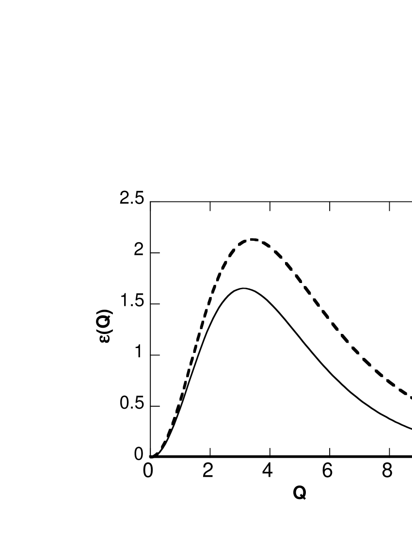
Figure 3: Energy-like scattering $\mathcal{E}\left({}^{\nu_{0},-\mathbf{Q}\ \ \nu_{0},\mathbf{0}}_{\,\,\nu_{0},\mathbf{Q}\ \ \ \nu_{0},\mathbf{0}}\right)$, given in eqs. (6.4) and (6.6), constructed on the dimensionless exchange parameter $\lambda\left({}^{n\ \,j}_{m\ i}\right)$ (see eq. (1.12)), for $m_{h}=m_{e}$, $m_{h}=2m_{e}$ and $m_{h}\gg m_{e}$ (same notations as in Fig.2).

We see from eq. (6.6) that $\mathcal{E}(Q)$ is equal to zero for $Q=0$ and $Q\rightarrow\infty$. We also see that it stays equal to zero for $\alpha_{e}=0$, i. e., for $m_{h}\gg m_{e}$. The numerical evaluation of $\tilde{\mathcal{E}}(\tilde{Q})$ for $m_{h}=m_{e}$ and $m_{h}=2m_{e}$ is shown in Fig.3.

As rederived in appendix D, this Pauli scattering $\mathcal{E}(Q)$ is nothing but the difference between the two exchange Coulomb scatterings, $\xi^{\mathrm{in}}(Q)-\xi^{\mathrm{out}}(Q)$, more precisely, the difference between their electron-hole contributions (see eq. (D.1)), since the electron-electron and hole-hole contributions to $\xi^{\mathrm{in}}$ and $\xi^{\mathrm{out}}$ are identical (see eq. (C.4)). Using eqs. (C.8,9), these partial contributions between different fermions read

$$\xi^{\mathrm{in}}_{\neq}(Q)=\xi^{\mathrm{out}}_{\neq}(Q)+\mathcal{E}(Q)=\xi^{\mathrm{in}}_{eh^{\prime}}\left({}^{\nu_{0},-\mathbf{Q}\ \ \nu_{0},\mathbf{0}}_{\,\,\nu_{0},\mathbf{Q}\ \ \ \nu_{0},\mathbf{0}}\right)+\xi^{\mathrm{in}}_{he^{\prime}}\left({}^{\nu_{0},-\mathbf{Q}\ \ \nu_{0},\mathbf{0}}_{\,\,\nu_{0},\mathbf{Q}\ \ \ \nu_{0},\mathbf{0}}\right)$$

$$=\sum_{\mathbf{k}}\left(2\varepsilon_{\nu_{0}}-\epsilon_{\mathbf{k}-\frac{\beta\mathbf{Q}}{2}}-\epsilon_{\mathbf{k}+\frac{\beta\mathbf{Q}}{2}}\right)\,\langle\nu_{0}|\mathbf{k}+\frac{\beta\mathbf{Q}}{2}\rangle\langle\nu_{0}|\mathbf{k}-\frac{\beta\mathbf{Q}}{2}\rangle\hskip 5.69046pt$$

$$\times\ \langle\mathbf{k}+\frac{\mathbf{Q}}{2}|\nu_{0}\rangle\langle\mathbf{k}-\frac{\mathbf{Q}}{2}|\nu_{0}\rangle\ .$$ (6.7)

Using the ground state wave function given in eq. (6.5), we can rewrite this scattering in Rydberg units as

$$\xi^{\mathrm{in}}_{\neq}(Q) = -\frac{e^{2}}{a_{X}}\,\left(\frac{a_{X}}{L}\right)^{2}\,\tilde{\xi}^{\mathrm{in}}_{\neq}(Qa_{X})$$

$$\tilde{\xi}^{\mathrm{in}}_{\neq}(\tilde{Q}) = \int_{0}^{+\infty}pdp\int_{0}^{2\pi}d\theta\,f(p,\theta;\beta\tilde{Q}/2)\,f(p,\theta;\tilde{Q}/2)\left[4+p^{2}+\frac{\beta^{2}\tilde{Q}^{2}}{4}\right]\ .$$ (6.8)

The partial “in” Coulomb scattering is shown in Fig.4 for $m_{h}=m_{e}$, $m_{h}=2m_{e}$ and $m_{h}\gg m_{e}$.

If we now turn to the electron-electron and hole-hole contributions to the exchange Coulomb scatterings $\xi^{\mathrm{in}}$ and $\xi^{\mathrm{out}}$, we find, using eq. (C.5), that the contribution coming from identical fermions is given by

$$\xi^{\mathrm{in}}_{=}(Q)=\xi^{\mathrm{out}}_{=}(Q)=\xi^{\mathrm{in}}_{ee}\left({}^{\nu_{0},-\mathbf{Q}\ \ \nu_{0},\mathbf{0}}_{\,\,\nu_{0},\mathbf{Q}\ \ \ \nu_{0},\mathbf{0}}\right)+\xi^{\mathrm{in}}_{hh}\left({}^{\nu_{0},-\mathbf{Q}\ \ \nu_{0},\mathbf{0}}_{\,\,\nu_{0},\mathbf{Q}\ \ \ \nu_{0},\mathbf{0}}\right)\hskip 156.49014pt$$

$$=\sum_{\mathbf{k}}\sum_{\mathbf{q}\neq\mathbf{0}}V_{\mathbf{q}}\langle\nu_{0}|\mathbf{k}+\frac{\beta\mathbf{Q}+\mathbf{q}}{2}\rangle\langle\nu_{0}|\mathbf{k}-\frac{\beta\mathbf{Q}+\mathbf{q}}{2}\rangle\hskip 159.3356pt$$

$$\times\left[\langle\mathbf{k}+\frac{\mathbf{Q}-\mathbf{q}}{2}|\nu_{0}\rangle\langle\mathbf{k}-\frac{\mathbf{Q}-\mathbf{q}}{2}|\nu_{0}\rangle+\langle\mathbf{k}+\frac{\mathbf{Q}+\mathbf{q}}{2}|\nu_{0}\rangle\langle\mathbf{k}-\frac{\mathbf{Q}+\mathbf{q}}{2}|\nu_{0}\rangle\right]\ .$$ (6.9)

In Rydberg units, this scattering reads as a fourth order integral

$$\xi^{\mathrm{in}}_{=}(Q) = \xi^{\mathrm{out}}_{=}(Q)=\frac{e^{2}}{a_{X}}\,\left(\frac{a_{X}}{L}\right)^{2}\,\tilde{\mathcal{E}}^{\mathrm{in}}_{=}(Qa_{X})$$

$$\tilde{\mathcal{E}}^{\mathrm{in}}_{=}(\tilde{Q}) = \int_{0}^{+\infty}pdp\int_{0}^{2\pi}d\theta\int_{0}^{+\infty}dr\,\int_{0}^{2\pi}\frac{d\theta^{\prime}}{2\pi}\,F(p,\theta;\frac{r}{2},\theta^{\prime};\frac{\beta\tilde{Q}}{2})$$

$$\hskip 85.35826pt\times\left[F(p,\theta;-\frac{r}{2},\theta^{\prime};\frac{\tilde{Q}}{2})+F(p,\theta;\frac{r}{2},\theta^{\prime};\frac{\tilde{Q}}{2})\right]$$

$$F(p,\theta;q,\theta^{\prime};K) = \left\{\left[1+\frac{p^{2}+K^{2}+q^{2}+2Kq\cos\theta^{\prime}}{4}\right]^{2}\right.\hskip 142.26378pt$$ (6.10)

$$\hskip 85.35826pt\left.-\left[\frac{pK\cos\theta+pq\cos(\theta-\theta^{\prime})}{2}\right]^{2}\right\}^{-3/2}.$$

Note that, for $q=0$, the function $F(p,\theta;q,\theta^{\prime};K)$ reduces to the function $f(p,\theta;K)$ entering $\tilde{\mathcal{E}}$ and $\tilde{\xi}^{\mathrm{in}}_{\neq}$.

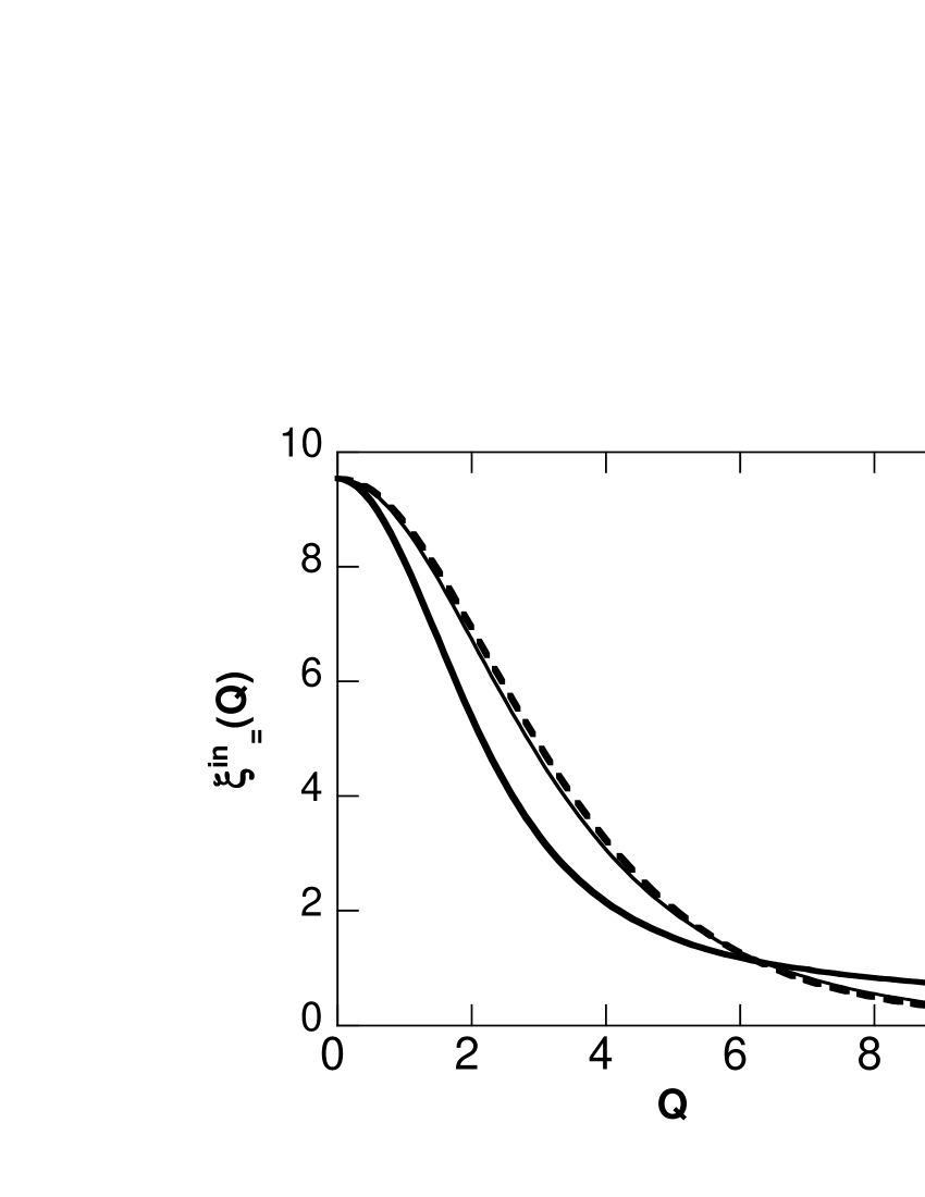
Figure 5: Contribution to the “in” Coulomb exchange scattering $\xi^{\mathrm{in}}_{=}\left({}^{\nu_{0},-\mathbf{Q}\ \ \nu_{0},\mathbf{0}}_{\,\,\nu_{0},\mathbf{Q}\ \ \ \nu_{0},\mathbf{0}}\right)$, coming from electron-electron and hole-hole interactions (see eqs. (6.9-10)), for $m_{h}\gg m_{e}$, $m_{h}=2m_{e}$ and $m_{h}=m_{e}$ (same notations as in Fig.2).

The numerical evaluation of the electron-electron and hole-hole contribution to the exchange Coulomb scattering is shown in Fig.5, for $m_{h}=m_{e}$, $m_{h}=2m_{e}$ and $m_{h}\gg m_{e}$.

From these two partial Coulomb exchange scatterings, we can obtain $\xi^{\mathrm{in}}(Q)$ through

$$\xi^{\mathrm{in}}(Q)=\xi^{\mathrm{in}}_{=}(Q)+\xi^{\mathrm{in}}_{\neq}(Q)\ ,$$ (6.11)

and $\xi^{\mathrm{out}}(Q)$ through

$$\xi^{\mathrm{out}}(Q)=\xi^{\mathrm{out}}_{=}(Q)+\xi^{\mathrm{out}}_{\neq}(Q)=\xi^{\mathrm{in}}(Q)-\mathcal{E}(Q)\ .$$ (6.12)

Note that $\xi^{\mathrm{in}}(Q)=\xi^{\mathrm{out}}(Q)$ for $\mathcal{E}(Q)=0$, i. e., for $Q=0$ and $Q\rightarrow\infty$, as well as for $m_{h}\gg m_{e}$ whatever the momentum transfer $Q$ is.

These two exchange scatterings are shown in Figs. 6 and 7. We see that they both cancel for a finite value of $Q$.

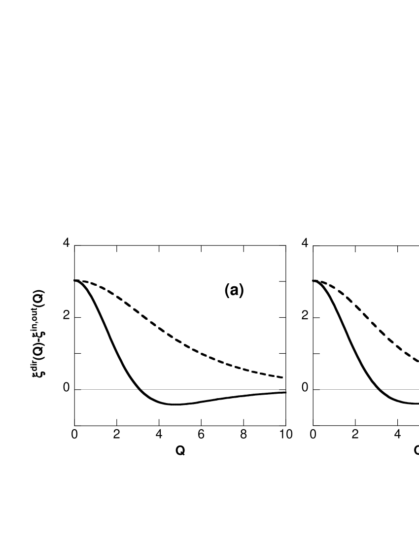
Figure 9: Solid line : effective scattering $\xi^{\mathrm{dir}}-\xi^{\mathrm{in}}$, which appears in the exact calculation of the transition rates of two excitons having same initial momentum, as a function of the momentum transfer $\mathbf{Q}$. Dashed line : effective scattering $\xi^{\mathrm{dir}}-\xi^{\mathrm{out}}$, as obtained from the effective bosonic Hamiltonian up to now used. Fig.(a) corresponds to $m_{h}=m_{e}$, while Fig.(b) corresponds to $m_{h}=2m_{e}$, the two effective scatterings being equal for $m_{h}\gg m_{e}$, as seen from eq. (6.12). The noticeable discrepancy between these effective scatterings questions the significance of the “very good agreement with experiments” obtained by using such effective bosonic scatterings, since in real experimental conditions, the exciton mass ratio $m_{h}/m_{e}$ is large but finite.

From these elementary scatterings between two cobosons, we can construct the two linear combinations of these scatterings appearing in the transition rates of two ground state excitons with same momentum, towards two ground state excitons with momentum $+\mathbf{Q}$ and $-\mathbf{Q}$, namely $\xi^{\mathrm{dir}}(Q)-\xi^{\mathrm{in}}(Q)$ as obtained through the many-body theory for composite excitons, and $\xi^{\mathrm{dir}}(Q)-\xi^{\mathrm{out}}(Q)$ as derived by the Haug and Schmitt-Rink incorrect effective Hamiltonian [2]. The correct effective scattering $\xi^{\mathrm{dir}}-\xi^{\mathrm{in}}$ is plotted in Fig.8 for $m_{h}=m_{e}$, $m_{h}=2m_{e}$ and $m_{h}\gg m_{e}$, while the two effective scatterings $\xi^{\mathrm{dir}}-\xi^{\mathrm{in}}$ and $\xi^{\mathrm{dir}}-\xi^{\mathrm{out}}$ are plotted in Fig.9, to allow an easy comparison of them. We see that these two effective scatterings have a similar behavior, as possible to guess from physical arguments, their values being however significantly different except for $m_{h}\gg m_{e}$. We also see that these effective scatterings both cancel for a finite value of the momentum transfer $Q$, the scattering rate of the associated process being then infinite. Let us stress that this somewhat unexpected result is obtained within the Born approximation — through the use of the Fermi golden rule. It might be specific to this approximation and disappear when higher order terms in Coulomb interaction are taken into account. However, it is also quite possible that this cancellation survives to all order in Coulomb interaction, since similar situations are known to occur, for example in atomic physics.

7 Conclusion

In the present work (paper I) on the exciton-exciton scattering, we concentrate on the importance of the exciton composite nature. We show that there is no way to get rid of this composite nature, by replacing the excitons by elementary bosons with Coulomb interaction dressed by carrier exchange, whatever is the way we dress it. For this purpose, we have here studied the problem of the lifetime and scattering rates of just two excitons, without spin degree of freedom.

While this paper is written in terms of excitons, the obtained results can be generalized to other composite bosons such as the ones found in cold gases much studied these days in atomic physics. Since the problems raised by replacing composite excitons by elementary excitons are generic, we are led to believe that fermion exchange between composite atoms should also play a significant role in the physics of these systems, as well as in the physics of other composite bosons.

The forthcoming paper II will be devoted to the importance of the spin degree of freedom in the scatterings of just two excitons and to the resulting polarization effects, since two bright excitons with opposite spins scatter into two dark excitons. Finally, paper III will study the many-body physics associated with these scatterings, through the time evolution of $N\gg 1$ excitons.

We wish to thank Marc-André Dupertuis for a careful study of the manuscript and his valuable comments.

APPENDICES

In previous works using our “commutation technique” for composite exciton interactions, we have obtained important results on the various scatterings between two excitons. The readers interested in this new many-body theory for cobosons can find useful to have them all rederived with coherent notations, some of the derivations we here give being actually simpler than the ones we first proposed.

Appendix A Exchange parameter

Using the exciton creation operator $B_{i}^{\dagger}$ in terms of free pairs given in eq. (1.1), the commutator of two composite exciton operators appears as

$$\left[B_{m},B_{i}^{\dagger}\right]=\sum_{\mathbf{p}_{e},\mathbf{p}_{h},\mathbf{k}_{e},\mathbf{k}_{h}}\langle\phi_{m}|\mathbf{p}_{e},\mathbf{p}_{h}\rangle\langle\mathbf{k}_{e},\mathbf{k}_{h}|\phi_{i}\rangle\left[b_{\mathbf{p}_{h}}a_{\mathbf{p}_{e}},a_{\mathbf{k}_{e}}^{\dagger}b_{\mathbf{k}_{h}}^{\dagger}\right]\ .$$ (A.1)

Since the commutator of two free pair operators is

$$\left[b_{\mathbf{p}_{h}}a_{\mathbf{p}_{e}},a_{\mathbf{k}_{e}}^{\dagger}b_{\mathbf{k}_{h}}^{\dagger}\right]=\delta_{\mathbf{p}_{e},\mathbf{k}_{e}}\,\delta_{\mathbf{p}_{h},\mathbf{k}_{h}}-\delta_{\mathbf{p}_{h},\mathbf{k}_{h}}\,a_{\mathbf{k}_{e}}^{\dagger}a_{\mathbf{p}_{e}}-\delta_{\mathbf{p}_{e},\mathbf{k}_{e}}\,b_{\mathbf{k}_{h}}^{\dagger}b_{\mathbf{p}_{h}}\ ,$$ (A.2)

the “deviation-from-boson operator” $D_{mi}$ defined in eq. (1.3), is given by

$$D_{mi}=\sum_{\mathbf{p}_{e},\mathbf{p}_{h},\mathbf{k}_{e},\mathbf{k}_{h}}\langle\phi_{m}|\mathbf{p}_{e},\mathbf{p}_{h}\rangle\langle\mathbf{k}_{e},\mathbf{k}_{h}|\phi_{i}\rangle\left(\delta_{\mathbf{p}_{h},\mathbf{k}_{h}}a_{\mathbf{k}_{e}}^{\dagger}a_{\mathbf{p}_{e}}+\delta_{\mathbf{p}_{e},\mathbf{k}_{e}}b_{\mathbf{k}_{h}}^{\dagger}b_{\mathbf{p}_{h}}\right)\ .$$ (A.3)

Using this expression of $D_{mi}$, we get

$$\left[D_{mi},B_{j}^{\dagger}\right]=\sum_{\mathbf{p}_{e},\mathbf{p}_{h},\mathbf{k}_{e},\mathbf{k}_{h},\mathbf{k}^{\prime}_{e},\mathbf{k}^{\prime}_{h}}\langle\phi_{m}|\mathbf{p}_{e},\mathbf{p}_{h}\rangle\langle\mathbf{k}_{e},\mathbf{k}_{h}|\phi_{i}\rangle\langle\mathbf{k}^{\prime}_{e},\mathbf{k}^{\prime}_{h}|\phi_{j}\rangle\hskip 85.35826pt$$

$$\times\ \left(\delta_{\mathbf{p}_{h},\mathbf{k}_{h}}\delta_{\mathbf{p}_{e},\mathbf{k}^{\prime}_{e}}a_{\mathbf{k}_{e}}^{\dagger}b_{\mathbf{k}^{\prime}_{h}}^{\dagger}+\delta_{\mathbf{p}_{e},\mathbf{k}_{e}}\delta_{\mathbf{p}_{h},\mathbf{k}^{\prime}_{h}}a_{\mathbf{k}^{\prime}_{e}}^{\dagger}b_{\mathbf{k}_{h}}^{\dagger}\right)\ .$$ (A.4)

If we now write the free pair operators in terms of exciton operators, according to

$$a_{\mathbf{k}_{e}}^{\dagger}b_{\mathbf{k}_{h}}^{\dagger}=\sum_{n}\langle\phi_{n}|\mathbf{k}_{e},\mathbf{k}_{h}\rangle\,B_{n}^{\dagger}\ ,$$ (A.5)

easy to check from eq. (1.1), we readily get eq. (1.2), in which we have set

$$\lambda\left({}^{n\ j}_{m\ i}\right) = \sum_{\mathbf{k}_{e},\mathbf{k}_{h},\mathbf{k}^{\prime}_{e},\mathbf{k}^{\prime}_{h}}\langle\phi_{m}|\mathbf{k}_{e},\mathbf{k}^{\prime}_{h}\rangle\,\langle\phi_{n}|\mathbf{k}^{\prime}_{e},\mathbf{k}_{h}\rangle\,\langle\mathbf{k}_{e},\mathbf{k}_{h}|\phi_{i}\rangle\,\langle\mathbf{k}^{\prime}_{e},\mathbf{k}^{\prime}_{h}|\phi_{j}\rangle$$ (A.6)

$$= \lambda\left({}^{m\ i}_{n\ j}\right)=\lambda\left({}^{j\ n}_{i\ m}\right)^{\ast}\ .$$

If we turn to real space, this equation gives the expression of $\lambda\left({}^{n\ j}_{m\ i}\right)$ given in eq. (1.4). Using it, with $\langle\mathbf{r}|\nu_{i}\rangle$ replaced by $\sum_{\mathbf{k}}\langle\mathbf{r}|\mathbf{k}\rangle\langle\mathbf{k}|\nu_{i}\rangle$, it is possible to write this exchange parameter in terms of the center-of-mass momenta and relative motion indices of the “in” and “out” excitons, as

$$\lambda\left({}^{\,\nu_{n},\mathbf{K}-\mathbf{p}-\mathbf{Q}\ \ \nu_{j},\mathbf{K}-\mathbf{p}}_{\nu_{m},\mathbf{K}+\mathbf{p}+\mathbf{Q}\ \ \nu_{i},\mathbf{K}+\mathbf{p}}\right)=\sum_{\mathbf{k}}\langle\nu_{m}|\mathbf{k}+\frac{\mathbf{P}_{-}}{2}\rangle\,\langle\nu_{n}|\mathbf{k}-\frac{\mathbf{P}_{-}}{2}\rangle\,\langle\mathbf{k}+\frac{\mathbf{P}_{+}}{2}|\nu_{i}\rangle\,\langle\mathbf{k}-\frac{\mathbf{P}_{+}}{2}|\nu_{j}\rangle\ ,$$ (A.7)

where $\mathbf{P}_{\pm}=2\alpha_{h}\mathbf{p}+(\alpha_{h}\pm\alpha_{e})\mathbf{Q}$. Note that this exchange parameter does not depend on the total center-of-mass momentum $2\mathbf{K}$ of the “in” and “out” excitons, as physically expected.

The link between $\lambda\left({}^{n\ j}_{m\ i}\right)$ and the possibility to form excitons with different pairs also appears if we couple the pairs of two excitons in different ways. Indeed, by using eq. (1.1), we find

$$B_{i}^{\dagger}B_{j}^{\dagger}=\sum_{\mathbf{k}_{e_{i}},\mathbf{k}_{e_{j}},\mathbf{k}_{h_{i}},\mathbf{k}_{h_{j}}}\langle\mathbf{k}_{e_{i}},\mathbf{k}_{h_{i}}|\phi_{i}\rangle\,\langle\mathbf{k}_{e_{j}},\mathbf{k}_{h_{j}}|\phi_{j}\rangle\ a_{\mathbf{k}_{e_{i}}}^{\dagger}b_{\mathbf{k}_{h_{i}}}^{\dagger}a_{\mathbf{k}_{e_{j}}}^{\dagger}b_{\mathbf{k}_{h_{j}}}^{\dagger}\ .$$ (A.8)

If we now use the free pair $a_{\mathbf{k}_{e_{i}}}^{\dagger}b_{\mathbf{k}_{h_{j}}}^{\dagger}$ to form the $m$ exciton and the free pair $a_{\mathbf{k}_{e_{j}}}^{\dagger}b_{\mathbf{k}_{h_{i}}}^{\dagger}$ to form the $n$ exciton, according to eq. (A.5) we get

$$B_{i}^{\dagger}B_{j}^{\dagger} = -\sum_{mn}B_{m}^{\dagger}B_{n}^{\dagger}\sum_{\mathbf{k}_{e_{i}},\mathbf{k}_{e_{j}},\mathbf{k}_{h_{i}},\mathbf{k}_{h_{j}}}\langle\mathbf{k}_{e_{i}},\mathbf{k}_{h_{i}}|\phi_{i}\rangle\langle\mathbf{k}_{e_{j}},\mathbf{k}_{h_{j}}|\phi_{j}\rangle\langle\phi_{m}|\mathbf{k}_{e_{i}},\mathbf{k}_{h_{j}}\rangle\langle\phi_{n}|\mathbf{k}_{e_{j}},\mathbf{k}_{h_{i}}\rangle$$ (A.9)

$$= -\sum_{mn}\lambda\left({}^{n\ j}_{m\ i}\right)\,B_{m}^{\dagger}B_{n}^{\dagger}=-\sum_{mn}\lambda\left({}^{m\ j}_{n\ i}\right)\,B_{m}^{\dagger}B_{n}^{\dagger}\ ,$$

since $B_{m}^{\dagger}B_{n}^{\dagger}=B_{n}^{\dagger}B_{m}^{\dagger}$.

Let us end this part on the exchange parameter by deriving a quite useful relation on a sum of $\lambda$’s. Starting from eq. (A.6) and using the closure relation for excitons, namely $\sum_{m}\langle\mathbf{p}_{e},\mathbf{p}_{h}|\phi_{m}\rangle\langle\phi_{m}|\mathbf{k}_{e},\mathbf{k}_{h}\rangle=\delta_{\mathbf{p}_{e},\mathbf{k}_{e}}\delta_{\mathbf{p}_{h},\mathbf{k}_{h}}$ and the one for free pairs, $\sum_{\mathbf{k}_{e},\mathbf{k}_{h}}\langle\phi_{p}|\mathbf{k}_{e},\mathbf{k}_{h}\rangle\langle\mathbf{k}_{e},\mathbf{k}_{h}|\phi_{i}\rangle=\delta_{pi}$, we immediately get equation (1.5), which shows that two hole exchanges reduce to an identity, as physically reasonable. This however has, as a bad consequence, the fact that counting the number of $\lambda$’s in a given quantity, does not amount to count the number of exchanges between the excitons involved.

Appendix B Direct Coulomb scattering

Let $H=H_{\mathrm{e}}+H_{\mathrm{h}}+\mathcal{V}_{\mathrm{ee}}+\mathcal{V}_{\mathrm{hh}}+\mathcal{V}_{\mathrm{eh}}$ be the semiconductor Hamiltonian. The commutator of the exciton creation operator $B_{i}^{\dagger}$ with the electron kinetic part gives

$$\left[H_{\mathrm{e}},B_{i}^{\dagger}\right]=\sum_{\mathbf{p},\mathbf{k}_{e},\mathbf{k}_{h}}\epsilon_{\mathbf{p}}^{(e)}\,\langle\mathbf{k}_{e},\mathbf{k}_{h}|\phi_{i}\rangle\,[a_{\mathbf{p}}^{\dagger}a_{\mathbf{p}},a_{\mathbf{k}_{e}}^{\dagger}b_{\mathbf{k}_{h}}^{\dagger}]=\sum_{\mathbf{k}_{e},\mathbf{k}_{h}}\epsilon_{\mathbf{k}_{e}}^{(e)}\,\langle\mathbf{k}_{e},\mathbf{k}_{h}|\phi_{i}\rangle\,a_{\mathbf{k}_{e}}^{\dagger}b_{\mathbf{k}_{h}}^{\dagger}\ ,$$ (B.1)

with a similar result for $H_{\mathrm{h}}$. The electron-hole Coulomb part gives

$$\left[\mathcal{V}_{\mathrm{eh}},B_{i}^{\dagger}\right]=-\sum_{\mathbf{p}_{e},\mathbf{p}_{h},\mathbf{k}_{e},\mathbf{k}_{h},\mathbf{q}}V_{\mathbf{q}}\,\langle\mathbf{k}_{e},\mathbf{k}_{h}|\phi_{i}\rangle\,[a_{\mathbf{p}_{e}+\mathbf{q}}^{\dagger}b_{\mathbf{p}_{h}-\mathbf{q}}^{\dagger}b_{\mathbf{p}_{h}}a_{\mathbf{p}_{e}},a_{\mathbf{k}_{e}}^{\dagger}b_{\mathbf{k}_{h}}^{\dagger}]\ ,$$ (B.2)

the commutator between free pairs being equal to

$$\left[a_{\mathbf{p}_{e}+\mathbf{q}}^{\dagger}b_{\mathbf{p}_{h}-\mathbf{q}}^{\dagger}b_{\mathbf{p}_{h}}a_{\mathbf{p}_{e}},a_{\mathbf{k}_{e}}^{\dagger}b_{\mathbf{k}_{h}}^{\dagger}\right]=\delta_{\mathbf{p}_{e},\mathbf{k}_{e}}\delta_{\mathbf{p}_{h},\mathbf{k}_{h}}\,a_{\mathbf{k}_{e}+\mathbf{q}}^{\dagger}b_{\mathbf{k}_{h}-\mathbf{q}}^{\dagger}\hskip 142.26378pt$$

$$+\delta_{\mathbf{p}_{e},\mathbf{k}_{e}}\,a_{\mathbf{k}_{e}+\mathbf{q}}^{\dagger}b_{\mathbf{k}_{h}}^{\dagger}b_{\mathbf{p}_{h}-\mathbf{q}}^{\dagger}b_{\mathbf{p}_{h}}+\delta_{\mathbf{p}_{h},\mathbf{k}_{h}}\,a_{\mathbf{k}_{e}}^{\dagger}b_{\mathbf{k}_{h}-\mathbf{q}}^{\dagger}a_{\mathbf{p}_{e}+\mathbf{q}}^{\dagger}a_{\mathbf{p}_{e}}\ .$$ (B.3)

To go further, we can note that, for excitons eigenstates of the semiconductor Hamiltonian, we have

$$H\,B_{i}^{\dagger}|v\rangle=(H_{\mathrm{e}}+H_{\mathrm{h}}+\mathcal{V}_{\mathrm{eh}})B_{i}^{\dagger}|v\rangle=[(H_{\mathrm{e}}+H_{\mathrm{h}}+\mathcal{V}_{\mathrm{eh}}),B_{i}^{\dagger}]|v\rangle=E_{i}\,B_{i}^{\dagger}|v\rangle\ ,$$ (B.4)

with $E_{i}=\Delta+\varepsilon_{\nu_{i}}+Q_{i}^{2}/2(m_{e}+m_{h})$, where $\Delta$ is the band gap ; so that, if we insert eqs. (B.1-3) into this eq. (B.4), we find that the $|\phi_{i}\rangle$’s are such that

$$(\epsilon_{\mathbf{k}_{e}}^{(e)}+\epsilon_{\mathbf{k}_{h}}^{(h)})\,\langle\mathbf{k}_{e},\mathbf{k}_{h}|\phi_{i}\rangle-\sum_{\mathbf{q}}V_{\mathbf{q}}\,\langle\mathbf{k}_{e}-\mathbf{q},\mathbf{k}_{h}+\mathbf{q}|\phi_{i}\rangle=E_{i}\,\langle\mathbf{k}_{e},\mathbf{k}_{h}|\phi_{i}\rangle\ .$$ (B.5)

Consequently, the commutator $[(H_{\mathrm{e}}+H_{\mathrm{h}}+\mathcal{V}_{\mathrm{eh}}),B_{i}^{\dagger}]|$ eventually reads

$$\left[(H_{\mathrm{e}}+H_{\mathrm{h}}+\mathcal{V}_{\mathrm{eh}}),B_{i}^{\dagger}\right]=E_{i}\,B_{i}^{\dagger}+V_{i}^{{\dagger}(eh)}\ ,$$ (B.6)

with $V_{i}^{{\dagger}(eh)}$ given by

$$V_{i}^{{\dagger}(eh)}=-\sum_{\mathbf{q},\mathbf{k}_{e},\mathbf{k}_{h}}V_{\mathbf{q}}\,\langle\mathbf{k}_{e},\mathbf{k}_{h}|\phi_{i}\rangle\,\left(a_{\mathbf{k}_{e}+\mathbf{q}}^{\dagger}b_{\mathbf{k}_{h}}^{\dagger}\sum_{\mathbf{p}_{h}}b_{\mathbf{p}_{h}-\mathbf{q}}^{\dagger}b_{\mathbf{p}_{h}}+a_{\mathbf{k}_{e}}^{\dagger}b_{\mathbf{k}_{h}-\mathbf{q}}^{\dagger}\sum_{\mathbf{p}_{e}}a_{\mathbf{p}_{e}+\mathbf{q}}^{\dagger}a_{\mathbf{p}_{e}}\right)\ .$$ (B.7)

In a similar way, we find

$$\left[\mathcal{V}_{\mathrm{ee}},B_{i}^{\dagger}\right]=V_{i}^{{\dagger}(ee)}=\sum_{\mathbf{q},\mathbf{k}_{e},\mathbf{k}_{h}}V_{\mathbf{q}}\,\langle\mathbf{k}_{e},\mathbf{k}_{h}|\phi_{i}\rangle\,a_{\mathbf{k}_{e}+\mathbf{q}}^{\dagger}b_{\mathbf{k}_{h}}^{\dagger}\sum_{\mathbf{p}_{e}}a_{\mathbf{p}_{e}-\mathbf{q}}^{\dagger}a_{\mathbf{p}_{e}}\ ,$$ (B.8)

$$\left[\mathcal{V}_{\mathrm{hh}},B_{i}^{\dagger}\right]=V_{i}^{{\dagger}(hh)}=\sum_{\mathbf{q},\mathbf{k}_{e},\mathbf{k}_{h}}V_{\mathbf{q}}\,\langle\mathbf{k}_{e},\mathbf{k}_{h}|\phi_{i}\rangle\,a_{\mathbf{k}_{e}}^{\dagger}b_{\mathbf{k}_{h}+\mathbf{q}}^{\dagger}\sum_{\mathbf{p}_{h}}b_{\mathbf{p}_{h}-\mathbf{q}}^{\dagger}b_{\mathbf{p}_{h}}\ .$$ (B.9)

So that we end with

$$\left[H,B_{i}^{\dagger}\right]=E_{i}\,B_{i}^{\dagger}+V_{i}^{\dagger}\ ,$$ (B.10)

$$V_{i}^{\dagger}=V_{i}^{{\dagger}(ee)}+V_{i}^{{\dagger}(hh)}+V_{i}^{{\dagger}(eh)}\ .$$ (B.11)

We now turn to the commutator of this creation potential with the exciton creation operator. From eqs. (B.8) and (1.1), we get

$$\left[V_{i}^{{\dagger}(ee)},B_{j}^{\dagger}\right]=\sum_{\mathbf{q},\mathbf{k}_{e},\mathbf{k}_{h},\mathbf{k}^{\prime}_{e},\mathbf{k}^{\prime}_{h}}V_{\mathbf{q}}\,\langle\mathbf{k}_{e},\mathbf{k}_{h}|\phi_{i}\rangle\langle\mathbf{k}^{\prime}_{e},\mathbf{k}^{\prime}_{h}|\phi_{j}\rangle\,a_{\mathbf{k}_{e}+\mathbf{q}}^{\dagger}b_{\mathbf{k}_{h}}^{\dagger}a_{\mathbf{k}^{\prime}_{e}-\mathbf{q}}^{\dagger}b_{\mathbf{k}^{\prime}_{h}}^{\dagger}\ .$$ (B.12)

We can rewrite the free pair operators $a_{\mathbf{k}_{e}+\mathbf{q}}^{\dagger}b_{\mathbf{k}_{h}}^{\dagger}$ and $a_{\mathbf{k}^{\prime}_{e}-\mathbf{q}}^{\dagger}b_{\mathbf{k}^{\prime}_{h}}^{\dagger}$ in terms of creation operators for $(m,n)$ excitons, according to eq. (A.5). This leads to

$$\left[V_{i}^{{\dagger}(ee)},B_{j}^{\dagger}\right]=\sum_{mn}\xi^{\mathrm{dir}}_{ee}\left({}_{m\ i}^{n\ j}\right)\,B_{m}^{\dagger}B_{n}^{\dagger}\ ,$$ (B.13)

where the direct Coulomb scattering due to electron-electron interaction is given by

$$\xi^{\mathrm{dir}}_{ee}\left({}_{m\ i}^{n\ j}\right)=\sum_{\mathbf{q},\mathbf{k}_{e},\mathbf{k}_{h},\mathbf{k}^{\prime}_{e},\mathbf{k}^{\prime}_{h}}V_{\mathbf{q}}\,\langle\mathbf{k}_{e},\mathbf{k}_{h}|\phi_{i}\rangle\langle\mathbf{k}^{\prime}_{e},\mathbf{k}^{\prime}_{h}|\phi_{j}\rangle\langle\phi_{m}|\mathbf{k}_{e}+\mathbf{q},\mathbf{k}_{h}\rangle\langle\phi_{n}|\mathbf{k}^{\prime}_{e}-\mathbf{q},\mathbf{k}^{\prime}_{h}\rangle\ .$$ (B.14)

If we go to real space, this scattering reads

$$\xi^{\mathrm{dir}}_{ee}\left({}_{m\ i}^{n\ j}\right)=\int d\mathbf{r}_{e}\,d\mathbf{r}_{e^{\prime}}\,d\mathbf{r}_{h}\,d\mathbf{r}_{h^{\prime}}\,\phi_{m}^{\ast}(\mathbf{r}_{e},\mathbf{r}_{h})\,\phi_{n}^{\ast}\mathbf{r}_{e^{\prime}},\mathbf{r}_{h^{\prime}})\,\phi_{i}(\mathbf{r}_{e},\mathbf{r}_{h})\,\phi_{j}(\mathbf{r}_{e^{\prime}},\mathbf{r}_{h^{\prime}})\,V_{ee^{\prime}}\ ,$$ (B.15)

where $V_{ee^{\prime}}=e^{2}/|\mathbf{r}_{e}-\mathbf{r}_{e^{\prime}}|=\sum_{\mathbf{q}}V_{\mathbf{q}}\,e^{i\mathbf{q}.(\mathbf{r}_{e}-\mathbf{r}_{e^{\prime}})}$ is the Coulomb interaction between the electrons $e$ and $e^{\prime}$. As for the exchange parameter, we can rewrite this scattering in terms of the center-of-mass momenta and relative motion indices as

$$\xi^{\mathrm{dir}}_{ee}\left({}^{\,\nu_{n},\mathbf{K}-\mathbf{p}-\mathbf{Q}\ \ \nu_{j},\mathbf{K}-\mathbf{p}}_{\nu_{m},\mathbf{K}+\mathbf{p}+\mathbf{Q}\ \ \nu_{i},\mathbf{K}+\mathbf{p}}\right) = V_{\mathbf{Q}}\sum_{\mathbf{k}_{i}}\langle\nu_{m}|\mathbf{k}_{i}+\alpha_{h}\mathbf{Q}\rangle\,\langle\mathbf{k}_{i}|\nu_{i}\rangle\sum_{\mathbf{k}_{j}}\langle\nu_{n}|\mathbf{k}_{j}-\alpha_{h}\mathbf{Q}\rangle\,\langle\mathbf{k}_{j}|\nu_{j}\rangle$$ (B.16)

$$= V_{\mathbf{Q}}\,\langle\nu_{m}|e^{i\alpha_{h}\mathbf{Q}.\mathbf{r}}|\nu_{i}\rangle\,\langle\nu_{n}|e^{-i\alpha_{h}\mathbf{Q}.\mathbf{r}}|\nu_{j}\rangle\ .$$

By using the same procedures for $V_{i}^{{\dagger}(hh)}$ and $V_{i}^{{\dagger}(eh)}$, it is easy to recover eq. (1.8), where, in real space, the direct Coulomb scattering between two excitons is given by eq. (1.9). In terms of the center-of-mass momenta and relative motion indices, this direct Coulomb scattering appears as

$$\xi^{\mathrm{dir}}\left({}^{\,\nu_{n},\mathbf{K}-\mathbf{p}-\mathbf{Q}\ \ \nu_{j},\mathbf{K}-\mathbf{p}}_{\nu_{m},\mathbf{K}+\mathbf{p}+\mathbf{Q}\ \ \nu_{i},\mathbf{K}+\mathbf{p}}\right)=V_{\mathbf{Q}}\langle\nu_{m}|e^{i\alpha_{h}\mathbf{Q}.\mathbf{r}}-e^{-i\alpha_{e}\mathbf{Q}.\mathbf{r}}|\nu_{i}\rangle\,\langle\nu_{n}|e^{-i\alpha_{h}\mathbf{Q}.\mathbf{r}}-e^{i\alpha_{e}\mathbf{Q}.\mathbf{r}}|\nu_{j}\rangle\ .$$ (B.17)

Note that $\xi^{\mathrm{dir}}$ depends neither on the total momentum $2\mathbf{K}$ of the “in” and “out” excitons, nor on the center-of-mass momenta of the “in” excitons separately, namely on $\mathbf{p}$, but just on the momentum transfer $\mathbf{Q}$.

We can note that, when one of the excitons stays unchanged, we have

$$\xi^{\mathrm{dir}}\left({}_{i\ i}^{n\ j}\right)=0\ ,$$ (B.18)

as can be seen by interchanging $e$ and $h$ in the integral of eq. (1.9). Indeed, $\phi_{i}^{\ast}(\mathbf{r}_{e},\mathbf{r}_{h})\phi_{i}(\mathbf{r}_{e},\mathbf{r}_{h})=|\langle\mathbf{r}_{e}-\mathbf{r}_{h}|\varphi_{\nu_{i}}\rangle|^{2}$ stays unchanged under this manipulation, whatever the parity of the relative motion wave function of the $i$ exciton is. This result physically comes from the fact that, in the case of excitons, the repulsion between identical fermions is as large as the attraction between different fermions. Let us stress that this property is no more valid for “cold atom” composite bosons, which only have an attractive part between different fermions in their interaction.

Appendix C Exchange Coulomb scatterings

From the direct Coulomb scatterings $\xi^{\mathrm{dir}}\left({}_{m\ i}^{n\ j}\right)$ and the exchange parameters $\lambda\left({}_{m\ i}^{n\ j}\right)$, we can construct two rather important exchange scatterings defined in eqs. (1.10) and (1.11), in which the carrier exchange takes place after or before the Coulomb interaction. By using eq. (1.5), it is easy to show that we also have

$$\xi^{\mathrm{dir}}\left({}_{m\ i}^{n\ j}\right) = \sum_{rs}\lambda\left({}_{m\ r}^{n\ s}\right)\,\xi^{\mathrm{in}}\left({}_{r\ i}^{s\ j}\right)\ ,$$ (C.1)

$$= \sum_{rs}\xi^{\mathrm{out}}\left({}_{m\ r}^{n\ s}\right)\,\lambda\left({}_{r\ i}^{s\ j}\right)\ .$$ (C.2)

From the definitions of $\lambda$ and $\xi^{\mathrm{dir}}$ in $\mathbf{r}$ space given in eqs. (1.4) and (1.9) and the fact that $\sum_{s}\phi_{s}^{\ast}(\mathbf{r}_{e_{1}},\mathbf{r}_{h_{1}})\phi_{s}(\mathbf{r}_{e_{2}},\mathbf{r}_{h_{2}})=\delta(\mathbf{r}_{e_{1}}-\mathbf{r}_{e_{2}})\,\delta(\mathbf{r}_{h_{1}}-\mathbf{r}_{h_{2}})$, it is easy to recover the expressions of $\xi^{\mathrm{in}}\left({}_{m\ i}^{n\ j}\right)$ and $\xi^{\mathrm{out}}\left({}_{m\ i}^{n\ j}\right)$ given in eqs. (1.10,11). These equations show that, while

$$\xi^{\mathrm{out}}\left({}_{m\ i}^{n\ j}\right)=\left[\xi^{\mathrm{in}}\left({}_{i\ m}^{j\ n}\right)\right]^{\ast}\ ,$$ (C.3)

we have for the contributions coming from $V_{ee^{\prime}}$ and $V_{hh^{\prime}}$ separately

$$\xi^{\mathrm{out}}_{cc^{\prime}}\left({}_{m\ i}^{n\ j}\right)=\xi^{\mathrm{in}}_{cc^{\prime}}\left({}_{m\ i}^{n\ j}\right)\ ,$$ (C.4)

with $c=e$ or $h$. This identity comes from the fact that the electron-electron and hole-hole scatterings are between both, the “in” and the “out” excitons, whatever the position of the carrier exchange is, while this is not true for the electron-hole parts. In terms of the center-of-mass momenta and relative motion indices, these $\xi^{\mathrm{in}}_{cc^{\prime}}$’s appear as

$$\xi^{\mathrm{in}}_{cc^{\prime}}\left({}^{\,\nu_{n},\mathbf{K}-\mathbf{p}-\mathbf{Q}\ \ \nu_{j},\mathbf{K}-\mathbf{p}}_{\nu_{m},\mathbf{K}+\mathbf{p}+\mathbf{Q}\ \ \nu_{i},\mathbf{K}+\mathbf{p}}\right)=\sum_{\mathbf{k}}\sum_{\mathbf{q}\neq\mathbf{0}}V_{\mathbf{q}}\langle\nu_{m}|\mathbf{k}+\frac{\mathbf{P}_{-}+\mathbf{q}}{2}\rangle\,\langle\nu_{n}|\mathbf{k}-\frac{\mathbf{P}_{-}+\mathbf{q}}{2}\rangle$$

$$\times\ \langle\mathbf{k}+\frac{\mathbf{P}_{+}\mp\mathbf{q}}{2}|\nu_{i}\rangle\,\langle\mathbf{k}-\frac{\mathbf{P}_{+}\mp\mathbf{q}}{2}|\nu_{j}\rangle\ ,$$ (C.5)

with the upper sign for $(ee^{\prime})$ and the lower sign for $(hh^{\prime})$, the momenta $\mathbf{P}_{\pm}$ being defined as for the exchange parameter $\lambda$ (see eq. (A.7)).

Similarly, the contributions to $\xi^{\mathrm{in}}$ coming from Coulomb interactions between electron and hole read

$$\xi^{\mathrm{in}}_{cd^{\prime}}\left({}^{\,\nu_{n},\mathbf{K}-\mathbf{p}-\mathbf{Q}\ \ \nu_{j},\mathbf{K}-\mathbf{p}}_{\nu_{m},\mathbf{K}+\mathbf{p}+\mathbf{Q}\ \ \nu_{i},\mathbf{K}+\mathbf{p}}\right)=-\sum_{\mathbf{k}}\sum_{\mathbf{q}\neq\mathbf{0}}V_{\mathbf{q}}\langle\nu_{m}|\mathbf{k}+\frac{\mathbf{P}_{-}+\mathbf{q}}{2}\rangle\,\langle\nu_{n}|\mathbf{k}-\frac{\mathbf{P}_{-}+\mathbf{q}}{2}\rangle$$

$$\times\ \langle\mathbf{k}+\frac{\mathbf{P}_{+}\mp\mathbf{q}}{2}|\nu_{i}\rangle\,\langle\mathbf{k}-\frac{\mathbf{P}_{+}\pm\mathbf{q}}{2}|\nu_{j}\rangle\ ,$$ (C.6)

with the upper sign for $(eh^{\prime})$ and the lower sign for $(he^{\prime})$.

It is of interest to note that, in these $\xi^{\mathrm{in}}_{cd^{\prime}}$, the sum over $\mathbf{q}$ can be readily done through

$$\epsilon_{\mathbf{k}}\,\langle\mathbf{k}|\nu\rangle-\sum_{\mathbf{q}}V_{\mathbf{q}}\,\langle\mathbf{k}+\mathbf{q}|\nu\rangle=\varepsilon_{\nu}\,\langle\mathbf{k}|\nu\rangle\ ,$$ (C.7)

with $\epsilon_{\mathbf{k}}=k^{2}/2\mu_{X}$ and $\mu_{X}^{-1}=m_{e}^{-1}+m_{h}^{-1}$, which follows from eq. (B.5). By setting $\mathbf{k}^{\prime}=\mathbf{k}-\mathbf{q}/2$, we then find

$$\xi^{\mathrm{in}}_{eh^{\prime}}\left({}^{\,\nu_{n},\mathbf{K}-\mathbf{p}-\mathbf{Q}\ \ \nu_{j},\mathbf{K}-\mathbf{p}}_{\nu_{m},\mathbf{K}+\mathbf{p}+\mathbf{Q}\ \ \nu_{i},\mathbf{K}+\mathbf{p}}\right)=\sum_{\mathbf{k}^{\prime}}(\varepsilon_{\nu_{m}}-\epsilon_{\mathbf{k}^{\prime}+\mathbf{P}_{-}/2})\,\langle\nu_{m}|\mathbf{k}^{\prime}+\frac{\mathbf{P}_{-}}{2}\rangle\,\langle\nu_{n}|\mathbf{k}^{\prime}-\frac{\mathbf{P}_{-}}{2}\rangle$$

$$\times\ \langle\mathbf{k}^{\prime}+\frac{\mathbf{P}_{+}}{2}|\nu_{i}\rangle\,\langle\mathbf{k}^{\prime}-\frac{\mathbf{P}_{+}}{2}|\nu_{j}\rangle\ .$$ (C.8)

In the same way, by setting $\mathbf{k}^{\prime}=\mathbf{k}+\mathbf{q}/2$, we find

$$\xi^{\mathrm{in}}_{he^{\prime}}\left({}^{\,\nu_{n},\mathbf{K}-\mathbf{p}-\mathbf{Q}\ \ \nu_{j},\mathbf{K}-\mathbf{p}}_{\nu_{m},\mathbf{K}+\mathbf{p}+\mathbf{Q}\ \ \nu_{i},\mathbf{K}+\mathbf{p}}\right)=\sum_{\mathbf{k}^{\prime}}(\varepsilon_{\nu_{n}}-\epsilon_{\mathbf{k}^{\prime}-\mathbf{P}_{-}/2})\,\langle\nu_{m}|\mathbf{k}^{\prime}+\frac{\mathbf{P}_{-}}{2}\rangle\,\langle\nu_{n}|\mathbf{k}^{\prime}-\frac{\mathbf{P}_{-}}{2}\rangle$$

$$\times\ \langle\mathbf{k}^{\prime}+\frac{\mathbf{P}_{+}}{2}|\nu_{i}\rangle\,\langle\mathbf{k}^{\prime}-\frac{\mathbf{P}_{+}}{2}|\nu_{j}\rangle\ .$$ (C.9)

Note that these eqs. (C.8) and (C.9) are similar to the expression (A.7) of the exchange parameter, except for the prefactors.

Appendix D Energy-like Pauli scattering

With $\lambda\left({}_{m\ i}^{n\ j}\right)$ alone, we can construct an energy-like scattering defined in eq. (1.12), which does not contain any Coulomb scattering between excitons explicitly. However, this $\mathcal{E}\left({}_{m\ i}^{n\ j}\right)$ scattering which seems to only rely on the composite boson character of the excitons through $\lambda\left({}_{m\ i}^{n\ j}\right)$, is nothing but the difference between the two exchange Coulomb scatterings, as written in eq. (1.13). In order to derive this relation, we write $\xi^{\mathrm{in}}\left({}_{m\ i}^{n\ j}\right)-\xi^{\mathrm{out}}\left({}_{m\ i}^{n\ j}\right)$, using eqs. (1.10,11). This leads to

$$\xi^{\mathrm{in}}\left({}_{m\ i}^{n\ j}\right)-\xi^{\mathrm{out}}\left({}_{m\ i}^{n\ j}\right)=\int d\mathbf{r}_{e}\,d\mathbf{r}_{e^{\prime}}\,d\mathbf{r}_{h}\,d\mathbf{r}_{h^{\prime}}\,\phi_{m}^{\ast}(\mathbf{r}_{e},\mathbf{r}_{h^{\prime}})\,\phi_{n}^{\ast}(\mathbf{r}_{e^{\prime}},\mathbf{r}_{h})\hskip 56.9055pt$$

$$\times\left[V_{eh}+V_{e^{\prime}h^{\prime}}-V_{eh^{\prime}}-V_{e^{\prime}h}\right]\,\phi_{i}(\mathbf{r}_{e},\mathbf{r}_{h})\,\phi_{j}(\mathbf{r}_{e^{\prime}},\mathbf{r}_{h^{\prime}})\ .$$ (D.1)

So that this difference only comes from electron-hole interactions, in agreement with the fact that the contribution from electron-electron or hole-hole interactions are similar for “in” and “out” Coulomb exchange scatterings (see eq. (C.4)).

By turning to $\mathbf{k}$ space, we find that the $V_{eh}$ term of the above equation reads

$$\int d\mathbf{r}_{e}\,d\mathbf{r}_{e^{\prime}}\,d\mathbf{r}_{h}\,d\mathbf{r}_{h^{\prime}}\,\phi_{m}^{\ast}(\mathbf{r}_{e},\mathbf{r}_{h^{\prime}})\,\phi_{n}^{\ast}(\mathbf{r}_{e^{\prime}},\mathbf{r}_{h})\,V_{eh}\,\phi_{i}(\mathbf{r}_{e},\mathbf{r}_{h})\,\phi_{j}(\mathbf{r}_{e^{\prime}},\mathbf{r}_{h^{\prime}})\hskip 113.81102pt$$

$$=\sum_{\mathbf{k}_{e},\mathbf{k}_{h},\mathbf{k}^{\prime}_{e},\mathbf{k}^{\prime}_{h},\mathbf{q}}V_{\mathbf{q}}\langle\phi_{m}|\mathbf{k}_{e},\mathbf{k}^{\prime}_{h}\rangle\langle\phi_{n}|\mathbf{k}^{\prime}_{e},\mathbf{k}_{h}\rangle\langle\mathbf{k}_{e}-\mathbf{q},\mathbf{k}_{h}+\mathbf{q}|\phi_{i}\rangle\langle\mathbf{k}^{\prime}_{e},\mathbf{k}^{\prime}_{h}|\phi_{j}\rangle\hskip 36.98866pt$$

$$=\sum_{\mathbf{k}_{e},\mathbf{k}_{h},\mathbf{k}^{\prime}_{e},\mathbf{k}^{\prime}_{h}}(\epsilon_{\mathbf{k}_{e}}^{(e)}+\epsilon_{\mathbf{k}_{h}}^{(h)}-E_{i})\langle\phi_{m}|\mathbf{k}_{e},\mathbf{k}^{\prime}_{h}\rangle\langle\phi_{n}|\mathbf{k}^{\prime}_{e},\mathbf{k}_{h}\rangle\langle\mathbf{k}_{e},\mathbf{k}_{h}|\phi_{i}\rangle\langle\mathbf{k}^{\prime}_{e},\mathbf{k}^{\prime}_{h}|\phi_{j}\rangle\ ,\hskip 14.22636pt$$ (D.2)

where we have used eq. (B.5). By calculating the $V_{e^{\prime}h^{\prime}}$ (resp. $V_{eh^{\prime}}$ and $V_{e^{\prime}h}$) term of eq. (D.1) in a similar way, we find that it reads as the last line of eq. (D.2) with the prefactor $(\epsilon_{\mathbf{k}_{e}}^{(e)}+\epsilon_{\mathbf{k}_{h}}^{(h)}-E_{i})$ replaced by $(\epsilon_{\mathbf{k}^{\prime}_{e}}^{(e)}+\epsilon_{\mathbf{k}^{\prime}_{h}}^{(h)}-E_{j})$ (resp. $(\epsilon_{\mathbf{k}_{e}}^{(e)}+\epsilon_{\mathbf{k}^{\prime}_{h}}^{(h)}-E_{m})$ and $(\epsilon_{\mathbf{k}^{\prime}_{e}}^{(e)}+\epsilon_{\mathbf{k}_{h}}^{(h)}-E_{n})$). By adding the four terms, we eventually get

$$\xi^{\mathrm{in}}\left({}_{m\ i}^{n\ j}\right)-\xi^{\mathrm{out}}\left({}_{m\ i}^{n\ j}\right) = (E_{m}+E_{n}-E_{i}-E_{j})$$ (D.3)

$$\times \sum_{\mathbf{k}_{e},\mathbf{k}_{h},\mathbf{k}^{\prime}_{e},\mathbf{k}^{\prime}_{h}}\langle\phi_{m}|\mathbf{k}_{e},\mathbf{k}^{\prime}_{h}\rangle\langle\phi_{n}|\mathbf{k}^{\prime}_{e},\mathbf{k}_{h}\rangle\langle\mathbf{k}_{e},\mathbf{k}_{h}|\phi_{i}\rangle\langle\mathbf{k}^{\prime}_{e},\mathbf{k}^{\prime}_{h}|\phi_{j}\rangle$$

$$= (E_{m}+E_{n}-E_{i}-E_{j})\,\lambda\left({}_{m\ i}^{n\ j}\right)=\mathcal{E}\left({}_{m\ i}^{n\ j}\right)\ .$$

Note that it is possible to recover this result directly from eqs. (C.3,4) and (C.8,9).

As a useful consequence of this eq. (D.3), the “in” and “out” exchange scatterings are equal if the energies of the “in” and “out” excitons are equal. This in particular shows that they are equal for diagonal processes:

$$\xi^{\mathrm{in}}\left({}_{i\ i}^{j\ j}\right)=\xi^{\mathrm{out}}\left({}_{i\ i}^{j\ j}\right)\ .$$ (D.4)

Appendix E Key equations to get correlation effects and time evolution of composite excitons

Correlation effects between composite excitons are obtained from the iteration of eq. (4.15). This equation follows from the commutator $[H,B_{i}^{\dagger}]$. Indeed, eq. (1.7) gives

$$H\,B_{i}^{\dagger}=B_{i}^{\dagger}(H+E_{i})+V_{i}^{\dagger}\ ,$$ (E.1)

so that

$$B_{i}^{\dagger}(a-H-E_{i})=(a-H)B_{i}^{\dagger}+V_{i}^{\dagger}\ .$$ (E.2)

If we now multiply this equation by $(a-H)^{-1}$ on the left and $(a-H-E_{i})^{-1}$ on the right, we readily get eq. (4.15).

Equation (4.15) can be used to obtain the time evolution of exciton states as an expansion in Coulomb scatterings. For that, we first note that

$$e^{-iHt}=-\int_{-\infty}^{+\infty}\frac{dx}{2i\pi}\,\frac{e^{-ixt}}{x-H+i\eta}\ ,$$ (E.3)

which is valid for any $t$ and $\eta$ $>0$. This is easy to check either by performing, in a formal way, the integration over the path made of the real axis $(-\infty,+\infty)$ and the lower infinite half circle, or by performing the same integration after having projected the operator at hand over a complete basis made of the $H$ eigenstates. This path goes around the pole $z=H-i\eta$, while it gives a negligible contribution over the circle $z=R\,e^{i\theta}$ for $-\pi<\theta<0$ and $R\rightarrow+\infty$, since $t>0$.

This leads to

$$e^{-iHt}\,B_{i}^{\dagger}=-\int_{-\infty}^{+\infty}\frac{dx}{2i\pi}\,\frac{e^{-ixt}}{x-H+i\eta}\ B_{i}^{\dagger}=-\int_{-\infty}^{+\infty}\frac{dx}{2i\pi}\,e^{-ixt}\left[B_{i}^{\dagger}\,\frac{1}{x-H-E_{i}+i\eta}\right.$$

$$+\left.\frac{1}{x-H+i\eta}\,V_{i}^{\dagger}\,\frac{1}{x-H-E_{i}+i\eta}\right]\ ,$$ (E.4)

due to eq. (4.15). From it, we readily recover eqs. (4.16,17), where the operator $W_{i}^{\dagger}(t)$ gives zero when acting on vacuum.

Figure 2: Direct Coulomb scattering $\xi^{\mathrm{dir}}\left({}^{\nu_{0},-\mathbf{Q}\ \ \nu_{0},\mathbf{0}}_{\,\,\nu_{0},\mathbf{Q}\ \ \ \nu_{0},\mathbf{0}}\right)$ given in eqs. (6.1) and (6.3) for two quantum well ground states excitons with same momentum taken as 0, scattered into two ground state excitons with momenta $(+\mathbf{Q})$ and $(-\mathbf{Q})$ for three values of $m_{h}/m_{e}$. Thick solid line: $m_{h}\gg m_{e}$; thin solid line: $m_{h}=2m_{e}$; thick dashed line: $m_{h}=m_{e}$. This plot, as all the other following plots, are done in reduced units, namely, $(e^{2}/a_{X})(a_{X}/L)^{2}$ for the scatterings and $a_{X}^{-1}$ for the momenta (see eq. 6.3)), $a_{X}$ being the 3D exciton Bohr radius.

Figure 4: Contribution to the “in” Coulomb exchange scattering $\xi^{\mathrm{in}}_{\neq}\left({}^{\nu_{0},-\mathbf{Q}\ \ \nu_{0},\mathbf{0}}_{\,\,\nu_{0},\mathbf{Q}\ \ \ \nu_{0},\mathbf{0}}\right)$, coming from electron-hole interactions (see eqs. (6.7-8)), for $m_{h}\gg m_{e}$, $m_{h}=2m_{e}$ and $m_{h}=m_{e}$ (same notations as in Fig.2).

Figure 6: “In” Coulomb exchange scattering $\xi^{\mathrm{in}}\left({}^{\nu_{0},-\mathbf{Q}\ \ \nu_{0},\mathbf{0}}_{\,\,\nu_{0},\mathbf{Q}\ \ \ \nu_{0},\mathbf{0}}\right)$, resulting from all Coulomb interactions between the “in” excitons (see eq. (6.11)), for $m_{h}\gg m_{e}$, $m_{h}=2m_{e}$ and $m_{h}=m_{e}$ (same notations as in Fig.2). Note that these scatterings cancel for a finite momentum transfer $\mathbf{Q}$.

Figure 7: “Out” Coulomb exchange scattering $\xi^{\mathrm{out}}\left({}^{\nu_{0},-\mathbf{Q}\ \ \nu_{0},\mathbf{0}}_{\,\,\nu_{0},\mathbf{Q}\ \ \ \nu_{0},\mathbf{0}}\right)$, resulting from all Coulomb interactions between the “out” excitons, for $m_{h}\gg m_{e}$, $m_{h}=2m_{e}$ and $m_{h}=m_{e}$ (same notations as in Fig.2). We see from Figs.6 and 7 that the “in” and “out” Coulomb exchange scatterings have similar behaviors while their precise values are different except for $m_{h}\gg m_{e}$ (thick solid line) or for zero momentum transfer $\mathbf{Q}$.

Figure 8: Effective scattering $\xi^{\mathrm{dir}}-\xi^{\mathrm{in}}$ appearing in the transition rate of two excitons with same initial momentum, as obtained from the many-body theory for composite excitons, for $m_{h}\gg m_{e}$, $m_{h}=2m_{e}$ and $m_{h}=m_{e}$ (same notations as in Fig.2). We see that this effective scattering cancels for a finite value of the momentum transfer $\mathbf{Q}$, this value depending on the mass ratio.

References

- [1] T. Usui, Prog. Theor. Phys. 23, 787 (1957).
- [2] H. Haug, S. Schmitt-Rink, Prog. Quantum Electron. 9, 3 (1984).
- [3] For a review, see A. Klein, E.R. Marshalek, Rev. Mod. Phys. 63, 375 (1991).
- [4] M. Combescot, O. Betbeder-Matibet, Europhys. Lett. 59, 579 (2002).
- [5] M. Combescot, O. Betbeder-Matibet, Phys. Rev. Lett. 93, 016403 (2004).
- [6] E. Hanamura, J. Phys. Soc. Jpn. 37, 1545 (1974).
- [7] J.N. Ginocchio, C.W. Johnson, Phys. Rev. C 51, 1861 (1995).
- [8] W. Schäfer, D.S. Kim, J. Shah, T.C. Damen, J.E. Cunningham, K.W. Goosen, L.N. Pfeiffer, K. Köhler, Phys. Rev. B 53, 16429 (1996).
- [9] J. Fernandez-Rossier, C. Tejedor, L. Munoz, L. Vina, Phys. Rev. B 54, 11582 (1996).
- [10] M. Kuwata-Gonokami, S. Inouye, H. Suzuura, M. Shirane, R. Shimano, Phys. Rev. Lett. 79, 1341 (1997).
- [11] J. Inoue, T. Brandes, A. Shimizu, J. Phys. Soc. Jpn. Lett. 67, 3384 (1998).
- [12] G. Rochat, C. Ciuti, V. Savona, C. Piermarocchi, A. Quattropani, P. Schwendimann, Phys. Rev. B 61, 13856 (2000).
- [13] S. Ben-Tabou, B. Laikhtman, Phys. Rev. B 63, 125306 (2001).
- [14] S. Okumura, T. Ogawa, Phys. Rev. B 65, 35105 (2001).
- [15] For a short review, see M. Combescot, O. Betbeder-Matibet, Solid State Com. 134, 11 (2005), and references therein.
- [16] A. Abrikosov, L. Gorkov, I. Dzyaloshinski, Methods of Quantum Field Theory in Statistical Physics, Prentice-Hall, Englewood Cliffs, NJ, 1963.
- [17] A. Fetter, J. Walecka, Quantum Theory of Many-particle Systems, McGraw-Hill, New York, 1971.
- [18] M. Combescot, O. Betbeder-Matibet, Europhys. Lett. 58, 87 (2002).
- [19] O. Betbeder-Matibet, M. Combescot, Eur. Phys. J. B 27, 505 (2002).
- [20] M. Combescot, O. Betbeder-Matibet, Phys. Rev. B 72, 193105 (2005).
- [21] D.B. Cassidy et al. , Phys. Rev. Lett. 95, 195006 (2005).
- [22] M. Combescot, O. Betbeder-Matibet, to appear in Eur. Phys. J. B.
- [23] M. Combescot, C. Tanguy, Europhys. Lett. 55, 390 (2001).
- [24] M. Combescot, X. Leyronas, C. Tanguy, Eur. Phys. J. B 31, 17 (2003).