Spin-dependent Rotating Wigner Molecules in Quantum dots

Abstract

The spin-dependent trial wave functions with rotational symmetry are introduced to describe rotating Wigner molecular states with spin degree of freedom in four- and five-electron quantum dots under magnetic fields. The functions are constructed with unrestricted Hartree-Fock orbits and projection technique in long-range interaction limit. They highly overlap with the exact-diagonalized ones and give the accurate energies in strong fields. The zero points, i.e. vortices of the functions have straightforward relations to the angular momenta of the states. The functions with different total spins automatically satisfy the angular momentum transition rules with the increase of magnetic fields and explicitly show magnetic couplings and characteristic oscillations with respect to the angular momenta. Based on the functions, it is demonstrated that the entanglement entropies of electrons depend on the z-component of total spin and rise with the increase of angular momenta.

I Introduction

The quantum dot systems, especially the few-electron dots with precise control of the particle number, have been extensively studied in recent years due to their abundant application potential and theoretical meaning. Experimentally, these systems are investigated as candidates for future quantum electronics, spintronicsWolf2001 and quantum information devicesLoss1998 ; Cerletti2005 . Theoretically, such two-dimensional (2D) confined systems with or without external fields have significant differences with the extent ones. In strong magnetic fields, the 2D electron gas with short-range interaction which exhibits the fractional quantum Hall effect has been understood based on the Laughlin and composite fermion wave functions.Laughlin1983 ; Jain1989 It is also anticipated that there will be the transition from the quantum liquid to the Wigner crystal in the magnetic fields corresponding to very small filling factors.Yang2001 ; Ye2002 ; Mandal2003 ; He2005 In quantum dots, it has been demonstrated that similar transition is much easier than that in extent systems due to the intrinsic long-range interactions.Yannouleas2003 ; Yannouleas2004 And both the exact-diagonalization method (ED) and the analytic theory confirm that the crystal states in quantum dots are not static but rotating ones with certain angular momenta, which are often referred to rotating Wigner molecules (RWMs).

In most investigations on few-electron states in quantum dots in strong magnetic fields, the spins of electrons are considered full-polarized and it simplifies the analytical theory and computational demands. However, in recent experiments, it has been possible to fabricate and study the quantum dots with negligible Zeeman splitting.Ellenberger2006 ; Salis2001 Then the full considerations of spin degree of freedom are needed and pose challenge to theorists. Although it has been demonstrated that the spin degree of freedom does not change the cystallization process in quantum dots, it will still bring new physical phenomena to the system.

In this work, we will introduce the four- and five-electron trial wave functions for the spin-dependent RWMs. Noticing that the similar four-electron wave function has been proposed recently by Jain et alJeon2007 and their results are consonant with our four-electron case, we will demonstrate that the functions highly agree with the ED results and concentrate on the different quantum characters between four and five electron quantum dots without the Zeeman splitting in strong magnetic fields. The remainder of the paper is organized as follows. The descriptions of the trial wave functions are introduced in Sec.II, the discussion of the accuracy of the functions and their quantum characters, such as the vortex numbers, magnetic couplings and entanglements between electrons are presented in Sec.III followed by a summary in Sec.IV.

II Wave Functions

In strong magnetic fields, unrestricted Hartree-Fock(UHF) orbits describing localized electrons can be approximated by displaced Gaussian functionsYannouleas2002

$$u(z,Z_{j})\!\!=\!\!\frac{1}{\sqrt{\pi}\lambda}\exp\!\!\left(-\frac{|z-Z_{j}|^{2}}{2\lambda^{2}}\right)\!\!\exp\!\!\left(\frac{zZ_{j}^{*}-z^{*}Z_{j}}{4l_{B}^{2}}\right)$$ (1)

where $\lambda=\sqrt{\hbar/m^{*}\Omega}$ , $\Omega=\sqrt{\omega_{0}^{2}+\omega_{c}^{2}/4}$ , $l_{B}=\sqrt{\hbar c/eB}$. $z=x-\mathrm{i}y$ is the complex coordinate of an electron. $Z_{j}=X_{j}+\mathrm{i}Y_{j}$ are the centers of the Gaussians and set to the positions of the equilibrium positions of electrons. The phase factor ensures the gauge invariance of each localized orbit. When $\omega_{0}=0$ or $\omega_{c}\gg\omega_{0}$, i.e. $\lambda=\sqrt{2}l_{B}$, $u(z,Z_{j})$ can be expanded to the first landau level

$$u(z,Z_{j})=\sum_{l=0}^{\infty}{c_{l}(Z_{j})\varphi_{l}(z)}$$ (2)

where $c_{l}(Z_{j})=(Z_{j}^{*}/\lambda)^{l}\exp(-|Z_{j}|^{2}/2\lambda^{2})/\sqrt{l!}$.

For a dot with $N_{1}$ spin-up and $N_{2}$ spin-down electrons ($N_{1}+N_{2}=N$), if the electrons form a RWM in a single ring configuration, we can construct $C_{N}^{N_{1}}$ many-body bases $|Z_{j_{1}}^{\uparrow},...,Z_{j_{N_{1}}}^{\uparrow},Z_{j_{N_{1}+1}}^{\downarrow},...,Z_{j_{N}}^{\downarrow}\rangle$ with z-component $S_{z}=(N_{1}-N_{2})/2$ from the localized UHF orbits centered at positions $Z_{1}\sim Z_{N}$ in clockwise, i.e. $Z_{j}=\exp(\mathrm{i}2\pi(1-j)/N)$. $\uparrow$ ($\downarrow$) represents the spin of the electron and each position can be only occupied by one particle with a certain spin.

Taking the four-electron case with $S_{z}=0$ as an example, the many-particle bases are

$$\left(\begin{array}[]{c}|1\rangle\\ |2\rangle\\ |3\rangle\\ |4\rangle\\ |5\rangle\\ |6\rangle\end{array}\right)=\left(\begin{array}[]{c}|Z_{1}^{\uparrow},Z_{2}^{\uparrow},Z_{3}^{\downarrow},Z_{4}^{\downarrow}\rangle\\ |Z_{1}^{\uparrow},Z_{3}^{\uparrow},Z_{2}^{\downarrow},Z_{4}^{\downarrow}\rangle\\ |Z_{1}^{\uparrow},Z_{4}^{\uparrow},Z_{2}^{\downarrow},Z_{3}^{\downarrow}\rangle\\ |Z_{2}^{\uparrow},Z_{3}^{\uparrow},Z_{1}^{\downarrow},Z_{4}^{\downarrow}\rangle\\ |Z_{2}^{\uparrow},Z_{4}^{\uparrow},Z_{1}^{\downarrow},Z_{3}^{\downarrow}\rangle\\ |Z_{3}^{\uparrow},Z_{4}^{\uparrow},Z_{1}^{\downarrow},Z_{2}^{\downarrow}\rangle\end{array}\right).$$ (3)

In the second quantization scheme, the N-electron Hamiltonian can be written as

$$H=\sum_{i}{\epsilon_{i}a_{i}^{+}a_{i}}+\frac{1}{2}\sum_{ijkl}{V_{ijkl}a_{i}^{+}a_{j}^{+}a_{l}a_{k}}.$$ (4)

The orbital energies and the direct Coulomb integrals of UHF orbits which are same for all bases and can be eliminated from the diagonal elements of $H$. If we assume that the exchange integrals between the neighbor electrons and next neighbors are $V_{ijji}=v_{1}$ and $V_{ikki}=v_{2}$, the Hamiltonian will have a simple form. For four electrons, it is

$$H=\left(\begin{array}[]{cccccc}-2v_{1}&v_{1}&-v_{2}&-v_{2}&v_{1}&0\\ v_{1}&-2v_{2}&v_{1}&v_{1}&0&v_{1}\\ -v_{2}&v_{1}&-2v_{1}&0&v_{1}&-v_{2}\\ -v_{2}&v_{1}&0&-2v_{1}&v_{1}&-v_{2}\\ v_{1}&0&v_{1}&v_{1}&-2v_{2}&v_{1}\\ 0&v_{1}&-v_{2}&-v_{2}&v_{1}&-2v_{1}\\ \end{array}\right).$$ (5)

The eigenstates of $(H,S^{2},S_{z})$ can be obtained by the diagonalization of $H$. The eigenvalues and eigenstates of Eq.(5) are

$$\begin{array}[]{lll}S=0&\left\{\begin{array}[]{l}E_{1}=2v_{1}-2v_{2}\\ E_{2}=2v_{2}-2v_{1}\end{array}\right.&\begin{array}[]{l}\psi_{1}:(1,2,1,1,2,1)\\ \psi_{2}:(1,0,-1,-1,0,1)\end{array}\\ S=1&\left\{\begin{array}[]{l}E_{3}=-2v_{1}\\ E_{4}=-2v_{1}\\ E_{5}=-2v_{2}\end{array}\right.&\begin{array}[]{l}\psi_{3}:(0,0,-1,1,0,0)\\ \psi_{4}:(-1,0,0,0,0,1)\\ \psi_{5}:(0,-1,0,0,1,0)\end{array}\\ S=2&\hskip 12.05553ptE_{6}=-4v_{1}-2v_{2}&\hskip 2.58334pt\psi_{6}:(1,-1,1,1,-1,1)\end{array}$$ (6)

Using Eq.(2), the many-particle bases can be expanded to the first Landau level as

$$|Z_{j_{1}}^{\uparrow},...,Z_{j_{N_{1}}}^{\uparrow},Z_{j_{N_{1}+1}}^{\downarrow},...,Z_{j_{N}}^{\downarrow}\rangle=\!\!\!\sum_{l_{1},l_{2},...,l_{N}=0}^{\infty}\!\!\!{c_{l_{1}}(Z_{j_{1}})c_{l_{2}}(Z_{j_{2}})...c_{l_{N}}(Z_{j_{N}})}{|l_{1}^{\uparrow},...,l_{N_{1}}^{\uparrow},l_{N_{1}+1}^{\downarrow},...,l_{N}^{\downarrow}\rangle}.$$ (7)

These many-particle bases are breaking symmetrical and contain the components of all angular momenta. The component of angular momentum $L$ can be obtained by projection operator techniqueYannouleas2002

$$|Z_{j_{1}}^{\uparrow},...,Z_{j_{N_{1}}}^{\uparrow},Z_{j_{N_{1}+1}}^{\downarrow},...,Z_{j_{N}}^{\downarrow}\rangle_{L}=\!\!\!\sum_{0\leq l_{1}<l_{2}<...<l_{N_{1}}\atop 0\leq l_{N_{1}+1}<...<l_{N}}^{l_{1}+l_{2}+...+l_{N}=|L|}\!\!\!{\det[c_{l_{1}}(Z_{j_{1}}),c_{l_{2}}(Z_{j_{2}}),...,c_{l_{N_{1}}}(Z_{j_{N_{1}}})]}$$

$${\det[c_{l_{N_{1}+1}}(Z_{j_{N_{1}+1}}),c_{l_{N_{1}+2}}(Z_{j_{N_{1}+2}}),...,c_{l_{N}}(Z_{j_{N}})]}{|l_{1}^{\uparrow},...,l_{N_{1}}^{\uparrow},l_{N_{1}+1}^{\downarrow},...,l_{N}^{\downarrow}\rangle}.$$ (8)

For four electrons again, they are (up to a constant)

$$|k\rangle_{L}\!\! =$$ (9)

$$\!\!\sum_{0\leq l_{1}<l_{2},0\leq l_{3}<l_{4}}^{l_{1}+l_{2}+l_{3}+l_{4}=|L|}{\!\!\left(\prod_{j=1}^{4}{l_{j}!}\right)^{-1/2}\!\!\!\!\!\!\!\!\left(\mathrm{i}^{kl_{2}}-\mathrm{i}^{kl_{1}}\right)\left(\mathrm{i}^{kl_{4}}-\mathrm{i}^{kl_{3}}\right)}$$

$$\!\!\times(-1)^{(l_{3}+l_{4})/k}|l_{1}^{\uparrow},l_{2}^{\uparrow},l_{3}^{\downarrow},l_{4}^{\downarrow}\rangle$$

where $k=1,2$, and

$$\begin{array}[]{ccr}|3\rangle_{L}&=&-\exp(\mathrm{i}6\pi|L|/4)|1\rangle_{L}\\ |4\rangle_{L}&=&-\exp(\mathrm{i}2\pi|L|/4)|1\rangle_{L}\\ |5\rangle_{L}&=&-\exp(\mathrm{i}2\pi|L|/4)|2\rangle_{L}\\ |6\rangle_{L}&=&\exp(\mathrm{i}4\pi|L|/4)|1\rangle_{L}\end{array}$$ (10)

due to the $\pi/2$ rotational symmetry of the positions $Z_{1}\sim Z_{4}$. Then six eigenstates with conserved angular momentum can be written as the linear combinations of $|1\rangle_{L}$ and $|2\rangle_{L}$ using the relations in Eq.(10). Since the phase differences in Eq.(10), for the states with a certain total spin, only those with proper $L$ have nonvanishing combination coefficients. The allowable $L$ and corresponding coefficients for the eigenstates are listed in Tab.1. It can be also recognized that $|1\rangle_{L}$ and $|2\rangle_{L}$ imply respectively the ferromagnetic and anti-ferromagnetic coupling between electrons. This fact will be important in following discussion of the properties of spin-dependent RWMs.

For five-electron case with $S_{z}=0.5$, repeat the same scheme and again for the two bases $|Z_{1}^{\uparrow},Z_{2}^{\uparrow},Z_{3}^{\uparrow},Z_{4}^{\downarrow},Z_{5}^{\downarrow}\rangle$ and $|Z_{1}^{\uparrow},Z_{2}^{\uparrow},Z_{4}^{\uparrow},Z_{3}^{\downarrow},Z_{5}^{\downarrow}\rangle$ which are ferromagnetic and ferrimagnetic, the components with angular momentum $L$ are respectively

$$|Z_{1}^{\uparrow},Z_{2}^{\uparrow},Z_{3}^{\uparrow},Z_{4}^{\downarrow},Z_{5}^{\downarrow}\rangle_{L}\!\!=$$

$$\!\!\sum_{0\leq l_{1}<l_{2}<l_{3},0\leq l_{4}<l_{5}}^{l_{1}+l_{2}+l_{3}+l_{4}+l_{5}=|L|}{\!\!\left(\prod_{j=1}^{5}{l_{j}!}\right)^{-1/2}}{\!\!\!\!\!\!\!\!\left(\delta^{l_{2}}-\delta^{l_{1}}\right)\left(\delta^{l_{3}}-\delta^{l_{2}}\right)}$$

$$\!\!\times\left(\delta^{l_{3}}-\delta^{l_{1}}\right)\left(\delta^{l_{5}}-\delta^{l_{4}}\right)\delta^{3(l_{4}+l_{5})}|l_{1}^{\uparrow},l_{2}^{\uparrow},l_{3}^{\uparrow},l_{4}^{\downarrow},l_{5}^{\downarrow}\rangle$$ (11)

$$|Z_{1}^{\uparrow},Z_{2}^{\uparrow},Z_{4}^{\uparrow},Z_{3}^{\downarrow},Z_{5}^{\downarrow}\rangle_{L}\!\!=$$

$$\!\!\sum_{0\leq l_{1}<l_{2}<l_{3},0\leq l_{4}<l_{5}}^{l_{1}+l_{2}+l_{3}+l_{4}+l_{5}=|L|}{\!\!\left(\prod_{j=1}^{5}{l_{j}!}\right)^{-1/2}}{\!\!\!\!\!\!\!\!\left(\delta^{l_{2}}-\delta^{l_{1}}\right)\left(\delta^{l_{3}}-\delta^{l_{2}}\right)}$$

$$\!\!\times\left(\delta^{l_{3}}-\delta^{l_{1}}\right)\left(\delta^{2l_{5}}-\delta^{2l_{4}}\right)\left(\delta^{l_{1}}+\delta^{l_{2}}+\delta^{l_{3}}\right)$$

$$\!\!\times\delta^{2(l_{4}+l_{5})}|l_{1}^{\uparrow},l_{2}^{\uparrow},l_{3}^{\uparrow},l_{4}^{\downarrow},l_{5}^{\downarrow}\rangle$$ (12)

where $\delta=\exp(\mathrm{i}\frac{2}{5}\pi)$. And at this time, there are ten eigenstates as the linear combinations of the two bases. See Tab.2 for corresponding coefficients.

Table 1: Eigenvalues, angular momenta, total spins, combination coefficients and magnetic couplings (MC) of the trial wave functions for four-electron spin-dependent RWMs

	$E$	$|L|$	$S$	$C_{1}$	$C_{2}$	MC
$\psi_{1}$	$2v_{1}-2v_{2}$	$4n+2$	0	1	1	1
$\psi_{2}$	$2v_{2}-2v_{1}$	$4n$	0	1	0	-1
$\psi_{3}$	$-2v_{1}$	$4n\pm 1$	1	1	0	-1
$\psi_{4}$	$-2v_{1}$	$4n\pm 1$	1	$\mp\mathrm{i}$	0	-1
$\psi_{5}$	$-2v_{2}$	$4n$	1	0	1	1
$\psi_{6}$	$-4v_{1}-2v_{2}$	$4n+2$	2	1	-0.5	0

Table 2: Eigenvalues, angular momenta, total spins, combination coefficients and magnetic couplings (MC) of the trial wave functions for five-electron spin-dependent RWMs

	$E$	$|L|$	$S$	$C_{1}$	$C_{2}$	MC
$\psi_{1}$	$-(v_{1}+v_{2})$	$5n$	0.5	1	1	0
$\psi_{2,3}$	$-(v_{1}+v_{2})-\sqrt{5}(v_{1}-v_{2})$	$5n\pm 2$	0.5	1	$\delta_{1}$	-1
$\psi_{4,5}$	$-(v_{1}+v_{2})+\sqrt{5}(v_{1}-v_{2})$	$5n\pm 1$	0.5	$\delta_{2}$	1	1
$\psi_{6,7}$	$-\frac{5}{2}(v_{1}+v_{2})-\frac{\sqrt{5}}{2}(v_{1}-v_{2})$	$5n\pm 1$	1.5	1	$\delta_{3}$	-1
$\psi_{8,9}$	$-\frac{5}{2}(v_{1}+v_{2})+\frac{\sqrt{5}}{2}(v_{1}-v_{2})$	$5n\pm 2$	1.5	$\delta_{4}$	1	1
$\psi_{10}$	$-5(v_{1}+v_{2})$	$5n$	2.5	1	-1	0

It is worthwhile to point out that the projection lead to the fact that not all the eigenstates with restored rotational symmetry are still orthogonal even if the breaking symmetrical ones do. It can be seen in Tab.1 that only five of six eigenstates are orthogonal. $\psi_{3}$ and $\psi_{4}$ are the same state up to a phase factor. The situation is similar in five-electron case as shown in Tab.2.

The scheme for constructing the trial functions with $S_{z}\neq 0(0.5)$ is same. Because in the following of the paper we will mainly discuss the RWMs with $S_{z}=0(0.5)$, the other wave functions are not shown here and will be attached in appendix.

Having got the eigenstates, we can evaluate their actual energies by considering the Hamiltonian of quantum dots with parabolic confinement and exact interactions as

$$H\!\!=\!\!\sum_{i=1}^{N}{\!\left(\frac{(\hat{P}_{i}\!+\!e\vec{A})^{2}}{2m_{e}^{*}}+\frac{1}{2}m_{e}^{*}\omega_{0}^{2}r_{i}^{2}\right)}\!\!+\!\!\sum_{i<j}{\frac{e^{2}}{4\pi\epsilon|\vec{r}_{i}-\vec{r}_{j}|}}$$ (13)

The energy expectation value ${\langle\psi|H|\psi\rangle}/{\langle\psi|\psi\rangle}$ of the trial function with angular momentum $L$ are

$$E_{dot}(B)=\frac{N}{2}\hbar\omega_{c}+(L+N)\hbar\frac{\omega_{0}^{2}}{\omega_{c}}+\frac{l_{0}}{l_{B}}\langle V\rangle$$ (14)

where $\langle V\rangle$ is the expectation value of interaction energy between electrons evaluated with $l_{B}$ equals to a certain length $l_{0}$.

Noticing that the overlap of a single-particle orbit $\varphi_{l}(z)$ in a quantum dot with the first Landau level $\varphi_{l}(z)_{\omega_{0}=0}$ is $[2\sqrt{2}\lambda\l_{B}/(\lambda^{2}+2l_{B}^{2})]^{|l|+1}$, we can also evaluate the overlap between the trial function with angular momentum $L$ and the exact-diagonalized one as

$$O_{L}=\left(\frac{2\sqrt{2}\lambda\l_{B}}{\lambda^{2}+2l_{B}^{2}}\right)^{|L|+N}\cdot(C_{T},C_{E})$$ (15)

where $(C_{T},C_{E})$ represents the inner product between the determinant coefficient vectors of trial function and that of exact-diagonalized one.

In order to study the quantum correlations in the trial functions, we can calculate the von Neumann entropiesPaskauskas2001 between an electron and the other part of the system as

$$S=-\mathrm{tr}(\rho^{f}\log_{2}\rho^{f})$$ (16)

where $\rho_{\mu,\nu}^{f}=\langle\psi|a_{\mu}^{+}a_{\nu}|\psi\rangle$ is the single-particle reduced density matrix.

III Disscussion

III.1 Energies, overlaps and vortices of the functions

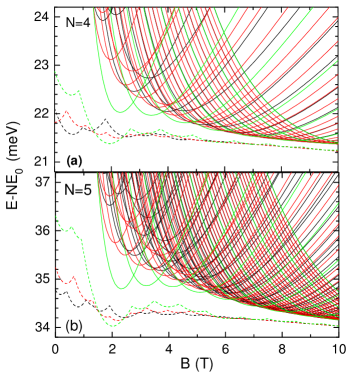
Figure 1: (Color online) Energy expectation values of the trial wave functions (solid lines) and the energy of the lowest states calculated by ED (dashed lines) for four (a) and five electrons (b) with total spins from the minimum to maximum values indicated by black, red and green lines, respectively. N times of the energy of the first Landau level have been subtracted from the total energy.

The energy expectation values of the trial functions obtained from Eq.(14) as function of magnetic field are plotted in Fig.1. In the same plot, we also present the energies of lowest states with different total spins calculated by ED. The ED calculations are executed beyond the lowest Landau level approximation and the confinement strength is set to 2meV. Then we employ the results of ED as a criterion to examine the accuracy of the trial functions. It can be seen in the plot that the results for four electrons obtained from the trial wave functions agree well with the ED ones in the magnetic field stronger than 5.7T with only an increase of the total energies lower than 0.25meV ($0.6\%$ of the total energy at $B=5.7T$). For five electrons, the difference is lower than 0.398meV (still $0.6\%$ of the total energy) when the field is stronger than 6T.

With the change of the field, both trial functions and ED exhibit accordant angular momentum transitions for the states with different total spins. In fact the allowable angular momenta of the trial functions listed in Tab.1 and 2 are just the angular momenta existing in the transitions identified by ED. When the magnetic field is strong enough, the trial functions can give correct energy sequence of different spin states and the values of the field where the transitions take place. In smaller fields, the full-polarized rotating Wigner molecules always have lower energies than the ones with other total spins if the states in quantum dots are described by the trial functions. However, the ED demonstrates that the states in small fields are actually liquidlike and the states which are not full-polarized can have lower energies. Then the trial functions cannot describe them correctly. It should be noticed that because the field ranges for liquid-to-crystal transition depend on the confinements of quantum dots, the trial functions can be expected to give better agreement with ED ones in smaller fields for the dot with weaker confinement.

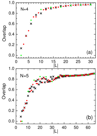
Figure 2: (Color online) Overlaps between the trial wave functions and ED ones for four (a) and five electrons (b) as function of angular momentum. $\times$, $\bullet$ and ▮ correspond to the states with non-, partial- to full-polarized spins, respectively.

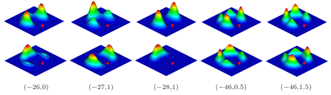
Figure 3: (Color online) Spin-dependent conditional probability densities of four-electron states with $(L,S)=(-26,0)$ $(-27,1)$ and (-28,1) and five-electron states $(-46,0.5)$ and $(-46,1.5)$ in QDs.The panels in the first(second) row show the distributions of the spin-down(up) electron. The red dots indicate the positions of the fixed spin-up electron.

Besides the energy expectation values, we also evaluate the overlaps between the trial functions and the ED ones. As shown in Fig.2, the higher overlaps convinced us that the trial functions can describe the states with larger angular momenta in quantum dots, i.e. the lowest states in strong field. The zero points, i.e. vortices of the many-body wave functions can reflect the charge distributions,Saarikoski2004 so we also inspect the vortex structures of the trial functions. The vortex number of the function just equals to the highest angular momentum occupied by the single particle. For four electron non-full-polarized states with $S_{z}=0$, the vortex number generally equals to $|L|-1$ as the function contains the component corresponds to the angular momentum distribution $\{l_{1},l_{2},l_{3},l_{4}\}=\{0,1,0,|L|-1\}$ or $\{l_{1},l_{2},l_{3},l_{4}\}=\{0,|L|-1,0,1\}$. An exception is the case when $|L|-1=4n$, where $n$ is an arbitrary integer. From Eq.(9) it can be found that the coefficient of such component is zero, so the vortex numbers of these states are $|L|-2$. For the full-polarized states, the vortex numbers are $|L|-3$ due to the Pauli exclusion principle. We also compare the vortex structures of the trial functions with that of ED ones. Although the angular momentum components of the trial functions are restricted in the first Landau level, the vortex number in the scope which contains the majority of the electron charge can agree well with the ED ones. Of course, due to the fact that our trial functions mainly reflect the long-range limit characters of the electrons in quantum dots, the vortex distributions are more dispersed and different from the ED ones.

For the energies, overlaps and vortices, the magnetic field or angular momentum beyond which the trial functions can get agreement with the ED ones for five electrons is larger than that for four-electron case. This is because that the transition from liquid to crystal states needs larger fields for the dots with larger particle numbers.

III.2 Spin correlations of RWMs

It has been pointed out in Sec.II that the many-body bases $|1\rangle_{L}$ and $|2\rangle_{L}$ for four-electron imply two species of magnetic coupling existing among electrons, respectively. Then the spin-dependent RWMs may also have corresponding properties since they are linear combinations of the two bases.

As listed in Tab.1, we have indicated the ferromagnetic, anti-ferromagnetic couplings and no specific coupling with number -1, 1 and 0 respectively. There are four-electron states like $\psi_{2\sim 5}$ which only contain the component $|1\rangle_{L}$ or $|2\rangle_{L}$ and of course they should have the corresponding type of magnetic coupling. There are also states like $\psi_{1}$ and $\psi_{5}$ containing both of the components. The full-polarized states $\psi_{6}$ should not have any specific magnetic coupling because the spin parts of the wave functions can be separated from the spatial parts. Then the states $\psi_{1}$ should have residual anti-ferromagnetic coupling because the ratio of the two components in them is different from that in $\psi_{6}$.

We also calculate the conditional probability densities (CPDs) of finding electrons with a certain species of spin to explicitly identify the two kind of magnetic couplings. As shown in Fig.3, if a spin-up electron is fixed, the remainder spin-up and -down electrons of four-electron state with $L=-27$, $S=1$ will be clearly at the neighbor and opposite positions, respectively. There are indeed the probability to find spin-down electrons at the neighbor positions. This is because the spin-down electrons have equal probability to stay at two remainder position if the spin-up electron is at left or right neighbor of the fixed ones. Such CPDs just reflect the ferromagnetic coupling between electrons. Then the other CPDs as the case of the state with $L=-28$, $S=1$ are the reflection of anti-ferromagnetic coupling. In these two examples, the states only contain the single component $|1\rangle_{L}$ or $|2\rangle_{L}$ respectively. The case of the state with $L=-26$, $S=0$ is also anti-ferromagnetic as the states with $L=-28$, $S=1$. However their CPDs have a slight difference since the state with $L=-26$, $S=0$ is just a sample of $\psi_{1}$ which contain both components $|1\rangle_{L}$ and $|2\rangle_{L}$.

Similar to the four-electron case, the five-electron bases Eq.(II) and Eq.(II) are ferromagnetic and ferrimagnetic respectively. Then the five-electron spin-dependent RWMs also have corresponding magnetic coupling as listed in Tab.2, where $-1$,1 and 0 respectively represent ferromagnetic, ferrimagnetic and no specific couplings. Different from the four-electron case, all of the five-electron RWMs contain both components of the two bases, they can only have the residual magnetic coupling if the ratios of the two components are different from that in full-polarized states $\psi_{10}$. The states like $\psi_{1}$ which have same ratio as $\psi_{10}$ also have no specific magnetic coupling. In Fig.3 we also show the CPDs of two five-electron states with $L=-46,S=0.5$ and $S=1.5$ which respectively reflect ferrimagnetic and ferromagnetic couplings.

Before the finish of the subsection, it is worthwhile to point out that there are regular magnetic coupling oscillations for spin-dependent RWMs with respect to the angular momentum which are in accordance with the electron molecules theory.Maksym2000 It can be identified in Tab.1 and 2 that with the increase of the angular momentum, the magnetic couplings of different spin states have periodic variations. We argue that these $L$-dependent spin correlations originate from that the configuration of localized UHF centers i.e. the classical position of electrons satisfies $2\pi/N$ rotational symmetry. The gauge invariance of the UHF orbits ensures the phase differences in Eq.(10) and results in the magnetic coupling oscillations. Therefore, we can conclude that these $L$-dependent spin correlations reflect the nature of spin-dependent RWMs.

III.3 $S_{z}$- and $L$-dependent entanglements

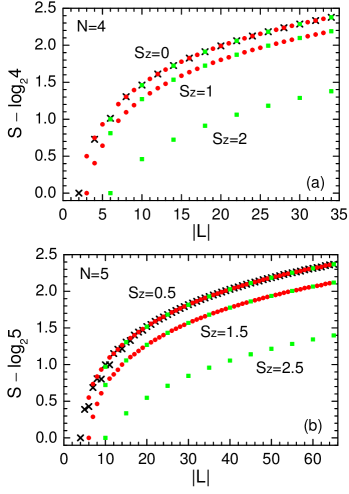
Figure 4: (Color online) Entanglement entropies of the trial wave functions of four (a) and five (b) electrons as function of angular momentum. $\times$, $\bullet$ and ▮ correspond to the states with non-, partial to full-polarized spins, respectively.

The rotating Wigner molecules are the states driven by strong particle correlation. When spin degree of freedom is considered, the correlation is naturally spin-dependent. The magnetic couplings discussed in the previous subsection are one kind of the reflection of such spin-dependent correlations.

Now we explore the entanglements of the trial functions which also reflect the quantum correlations existing in RWMs. The von Neumann entropy is used for evaluating the entanglement between one electron and the other part of the system. In the case of identical particles, the exchange symmetry of wave functions contributes a constant $\log_{2}N$ to the total entropies. Such parts of the entropies do not reflect the entanglements we concern, so we extract them from the total entropies and the corresponding results are shown in Fig.4, which not only contain the states with $S_{z}=0(0.5)$ but also the ones with $S_{z}=1(1.5)$ and $2(2.5)$. The entropies given by the trial functions show that the entanglements of RWMs increase monotonously with the increase of the angular momentum. For a given $L$, the states with different $S$ but same $S_{z}$ have almost equal entanglement, especially when $|L|$ is large enough. For the states with same $S$ but different $S_{z}$, the entropies will have a constant difference. For the states with largest $S_{z}$, since all electrons have same spin, there are no entanglements originating from spin components and the entropies will differ from that of the states with smallest $S_{z}$ by one.

IV Summary

In summary, a set of trial wave functions for describing the spin-dependent rotating Wigner molecular states is constructed from the localized unrestricted Hartree-Fock orbits with the assumed long-range interaction. The projection operator technique is employed to restore the rotational symmetry. By examining the energies of the functions and their overlaps with the exact-diagonalized ones with the full consideration of the interactions, it is demonstrated that the trial functions are suitable for the studies of the few-electron states of quantum dots in strong magnetic fields. The vortex numbers of the functions are generally $|L|-1$ for the non-full-polarized states with $S_{z}=0$, where $|L|$ is the angular momentum of the state, except the states with $|L|-1=4n$ whose vortex numbers are $|L|-2$. They automatically satisfy correct angular momentum transition rules of different spin states with the increase of the magnetic fields. These functions explicitly show that there are ferromagnetic and anti-ferromagnetic couplings between electrons in four-electron rotating Wigner moleculars, and ferromagnetic and ferrimagnetic couplings in five-electron case. The different spin states have specific magnetic coupling oscillation patterns with the change of angular momentum. The allowable angular momenta and the $L$-dependent magnetic coupling of different spin states are caused by the $2\pi/N$ rotational symmetry of the classical positions of electrons and reflect the nature of spin-dependent rotating Wigner moleculars. It is also shown that the entanglements i.e. the quantum correlations of the states increase monotonously with the increase of angular momentum. The states with different $S$ but same $S_{z}$ have similar entanglement entropies. The entropy differences of the states with different $S_{z}$ are approximately constant in strong magnetic fields. These trial functions will be useful in future studies of the few-electron states and their quantum behaviors in quantum dots in strong magnetic fields.

Appendix: Situations for $S_{z}\neq 0(0.5)$

For four-electron RWMs with $S_{z}=1$, the many-body bases are

$$\left(\begin{array}[]{c}|1\rangle^{\prime}\\ |2\rangle^{\prime}\\ |3\rangle^{\prime}\\ |4\rangle^{\prime}\end{array}\right)=\left(\begin{array}[]{c}|Z_{1}^{\uparrow},Z_{2}^{\uparrow},Z_{3}^{\uparrow},Z_{4}^{\downarrow}\rangle\\ |Z_{1}^{\uparrow},Z_{2}^{\uparrow},Z_{4}^{\uparrow},Z_{3}^{\downarrow}\rangle\\ |Z_{1}^{\uparrow},Z_{3}^{\uparrow},Z_{4}^{\uparrow},Z_{2}^{\downarrow}\rangle\\ |Z_{2}^{\uparrow},Z_{3}^{\uparrow},Z_{4}^{\uparrow},Z_{1}^{\downarrow}\rangle\end{array}\right).$$ (17)

Examining the CPDs or noticing that there is only one spin-down electron, it can be found that the electrons in these bases have no specific magnetic coupling.

The corresponding Hamiltonian is

$$H=\left(\hskip 4.30554pt\begin{array}[]{cccc}-2v_{1}-v_{2}&v_{1}&-v_{2}&v_{1}\\ v_{1}&-2v_{1}-v_{2}&v_{1}&-v_{2}\\ -v_{2}&v_{1}&-2v_{1}-v_{2}&v_{1}\\ v_{1}&-v_{2}&v_{1}&-2v_{1}-v_{2}\end{array}\hskip 4.30554pt\right).$$ (18)

The eigenvalues and eigenstates of $(H,S^{2},S_{z})$ are

$$\begin{array}[]{lll}S=1&\left\{\begin{array}[]{l}E_{1^{\prime}}=-2v_{1}\\ E_{2^{\prime}}=-2v_{1}\\ E_{3^{\prime}}=-2v_{2}\end{array}\right.&\begin{array}[]{l}\psi_{1^{\prime}}:(-1,0,1,0)\\ \psi_{2^{\prime}}:(0,-1,0,1)\\ \psi_{3^{\prime}}:(1,1,1,1)\end{array}\\ \\ S=2&\hskip 12.05553ptE_{4^{\prime}}=-4v_{1}-2v_{2}&\hskip 2.58334pt\psi_{4^{\prime}}:(1,-1,1,-1).\end{array}$$ (19)

It can be found that the states with $S_{z}=1$ have same energies as the ones with $S_{z}=0$ and same $S$.

Again, we expand $|1\rangle^{\prime}$ to the first Landau level and then the component with angular momentum $L$ is

$$|1\rangle^{\prime}_{L}\!\! =$$ (20)

$$\!\!\sum_{0\leq l_{1}<l_{2}<l_{3},0\leq l_{4}}^{l_{1}+l_{2}+l_{3}+l_{4}=|L|}{\!\!\left(\prod_{j=1}^{4}{l_{j}!}\right)^{-1/2}\!\!\!\!\!\!\!\!\left(\mathrm{i}^{l_{2}}-\mathrm{i}^{l_{1}}\right)\left(\mathrm{i}^{l_{3}}-\mathrm{i}^{l_{2}}\right)}$$

$$\!\!\times\left(\mathrm{i}^{l_{3}}-\mathrm{i}^{l_{1}}\right)(-\mathrm{i})^{l_{4}}|l_{1}^{\uparrow},l_{2}^{\uparrow},l_{3}^{\uparrow},l_{4}^{\downarrow}\rangle,$$

and there are relations as follows

$$\begin{array}[]{ccc}|2\rangle^{\prime}_{L}&=&\exp(\mathrm{i}6\pi|L|/4)|1\rangle^{\prime}_{L}\\ |3\rangle^{\prime}_{L}&=&\exp(\mathrm{i}4\pi|L|/4)|1\rangle^{\prime}_{L}\\ |4\rangle^{\prime}_{L}&=&\exp(\mathrm{i}2\pi|L|/4)|1\rangle^{\prime}_{L}\end{array}.$$ (21)

Using Eq.(21), four eigenstates in Eq.(19) with restored rotational symmetry can be obtained. For the states with $S=1$, only those with $|L|=4k\pm 1$ or $|L|=4k$ are allowable. For the states with $S=2$, only those with $|L|=4k+2$ are nonvanishing. These angular momentum rules are same as the ones for the states with $S_{z}=0$. Of course these states do not have any specific magnetic coupling.

Similarly, it can be obtained that the five-electron RWMs with $S_{z}=1.5$ have same energies and angular momentum rules as the ones with $S_{z}=0.5$. They can be represented by the many-body basis (up to a phase factor)

$$|Z_{1}^{\uparrow},Z_{2}^{\uparrow},Z_{3}^{\uparrow},Z_{4}^{\uparrow},Z_{5}^{\downarrow}\rangle_{L}\!\!=$$

$$\!\!\sum_{0\leq l_{1}<l_{2}<l_{3}<l_{4},0\leq l_{5}}^{l_{1}+l_{2}+l_{3}+l_{4}+l_{5}=|L|}{\!\!\left(\prod_{j=1}^{5}{l_{j}!}\right)^{-1/2}}{\!\!\!\!\!\!\!\!\prod_{i<j}{\left(\delta^{l_{j}}-\delta^{l_{i}}\right)}}$$

$$\!\!\times\delta^{4l_{5}}|l_{1}^{\uparrow},l_{2}^{\uparrow},l_{3}^{\uparrow},l_{4}^{\uparrow},l_{5}^{\downarrow}\rangle.$$ (22)

And they also have no specific magnetic coupling.

Finally, the wave functions for full-polarized RWMs with largest $S_{z}$ can be found in other referencesYannouleas2004 and are no longer discussed here.

References

• (1) S. A. Wolf, D. D. Awschalom, R. A. Buhrman, J. M. Daughton, S. von Molnár, M. L. Roukes, A. Y. Chtchelkanova and D. M. Treger, Science 294, 1488 (2001).
• (2) D.Loss and D. P. DiVincenzo, Phys. Rev. A 57, 120 (1998).
• (3) V. Cerletti, W. A. Coish, O. Gywat and D. Loss, Nanotechnology 16, R27 (2005).
• (4) R. B. Laughlin, Phys. Rev. Lett. 50, 1395 (1983).
• (5) J. K. Jain, Phys. Rev. Lett. 63, 199 (1989).
• (6) K. Yang, F. D. M. Haldane and E. H. Rezayi, Phys. Rev. B 64, 081301 (2001).
• (7) P. D. Ye, L.W. Engel, D. C. Tsui, R.M. Lewis, L. N. Pfeiffer and K.West, Phys. Rev. Lett. 89, 176802 (2002).
• (8) S. S. Mandal, M. R. Peterson and J. K. Jain, Phys. Rev. Lett. 90, 106403 (2003).
• (9) W. J. He, T. Cui, Y. M. Ma, C. B. Chen, Z. M. Liu, and G. T. Zou, Phys. Rev. B 72, 195306 (2005).
• (10) C. Yannouleas and U. Landman, Phys Rev B 68, 035326 (2003).
• (11) C. Yannouleas and U. Landman, Phys Rev B 70, 235319 (2004).
• (12) C. Yannouleas and U. Landman, Phys Rev B 66, 115315 (2002).
• (13) C. Ellenberger, T. Ihn, C. Yannouleas, U. Landman, K. Ensslin, D. Driscoll and A. C. Gossard Phys. Rev. Lett. 96, 126806 (2006).
• (14) G. Salis, Y. Kato, K. Ensslin, D. C. Driscoll, A. C. Gossard and D. D. Awschalom Nature. 414, 619 (2001).
• (15) C. Shi, G. S. Jeon, and J. K. Jain, Phys. Rev. B 75, 165302 (2007).
• (16) R. Paškauskas and L. You, Phys. Rev. A 64, 042310 (2001).
• (17) H. Saarikoski, A. Harju, M. J. Puska, and R.M. Nieminen, Phys. Rev. Lett. 93, 116802 (2004).
• (18) P. A. Maksym, H. Imamura, G. P. Mallon, and H. Aoki, J. Phys.:Condens. Matter 12, R299 (2000).