Perfectly Conducting Channel and Universality Crossover in Disordered Nano-Graphene Ribbons

Abstract

The band structure of graphene ribbons with zigzag edges have two valleys well separated in momentum space, related to the two Dirac points of the graphene spectrum. The propagating modes in each valley contain a single chiral mode originating from a partially flat band at band center. This feature gives rise to a perfectly conducting channel in the disordered system, if the impurity scattering does not connect the two valleys, i.e. for long-range impurity potentials. Ribbons with short-range impurity potentials, however, through inter-valley scattering display ordinary localization behavior. The two regimes belong to different universality classes: unitary for long-range impurities and orthogonal for short-range impurities.

The recent fabrication of graphene devices, combined with observation of half-integer quantum Hall effectnovoselov and the intrinsic $\pi$-phase shift of the Shubnikov-de Haas oscillationskopelvich , has once more ignited an intense discussion on this old fascinating system. Due to the two-dimensional honeycomb structure, the itinerant $\pi$-electrons near the Fermi energy behave as massless Dirac fermion. The valence and conduction bands touch conically at two nonequivalent Dirac points, called $\bm{K_{+}}$ and $\bm{K_{-}}$ points, which possess opposite chirality chiral .

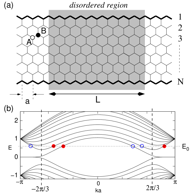
Figure 1: (a) Structure of graphene zigzag ribbon. The disordered region with randomly distributed impurites lies in the shaded region and has the length $L$. The lattice constant is $a$ and the ribbon width $N$ is defined as the number of the zigzag chains. (b) Energy dispersion of zigzag ribbon with $N=10$. The valleys in the energy dispersion near $k=2\pi/3a$ ($k=-2\pi/3a$) originate from the Dirac $\bm{K_{+}}$($\bm{K_{-}}$)-point of graphene. The red-filled (blue-unfilled) circles denote the right (left)-moving open channel at the energy $E_{0}$. In the left(right) valley separately the degeneracy between right and left moving channels is missing due to one excess right(left)-going mode. The time-reversal symmetry under the intra-valley scattering is also broken.

In graphene, the presence of edges can have strong implications for the spectrum of the $\pi$-electrons peculiar . There are two basic shapes of edges, armchair and zigzag which determine the properties of graphene ribbons. In ribbons with zigzag edges, localized states appear at the edge with energies close to the Fermi level peculiar . In contrast, edge states are absent for ribbons with armchair edges. Recent experiments support the evidence of edge localized statesenoki . The electronic transport through zigzag ribbons shows a number of intriguing phenomena such as zero-conductance Fano resonances prl , vacancy configuration dependent transport vacancy , valley filtering rycerz and half-metallic conduction son .

In this Letter, we focus on disorder effects of the electronic transport properties of graphene zigzag ribbons. The edge states play an important role here, since they appear as special modes with partially flat bands and lead under certain conditions to chiral modes. There is one such mode of opposite orientation in each of the two valleys, which are well separated in $k$-space. The key result of this study is that for disorder without inter-valley scattering a single perfectly conducting channel emerges associated with such a chiral mode. This mode disappears as soon as inter-valley scattering is possible. This distinction depends on the range of the impurity potentials. We will show that as a function of the impurity potential range a crossover from the orthogonal to the unitary universality class occurs which is connected with the presence or absence of time reversal symmetry (TRS).

We describe the electronic states of nanographites by the tight-binding model

$$H=\sum_{i,j}\gamma_{i,j}|i\rangle\langle j|+\sum_{i}V_{i}|i\rangle\langle i|,$$ (1)

where $\gamma_{i,j}=-1$ if $i$ and $j$ are nearest neighbors, and 0 otherwise. $|i\rangle$ represents the state of the $p_{z}$-orbital on site $i$ neglecting the spin degrees of freedom. In the following we will also apply magnetic fields perpendicular to the graphite plane which are incorporated via the Peierls phase: $\gamma_{i,j}\rightarrow\gamma_{i,j}\exp\left[i2\pi(e/ch)\int_{i}^{j}d\bm{l\cdot A}\right]$, where $\bm{A}$ is the vector potential. The second term in Eq. (1) represents the impurity potential, $V_{i}=V(\bm{r}_{i})$ is the impurity potential at a position $\bm{r}_{i}$.

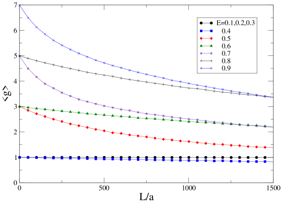
Figure 2: $L$-dependence of the average of dimensionless conductance $\langle g\rangle$ for zigzag ribbon with $N=10$, $d/a=1.5$ (no inter-valley scattering), $u_{0}=1.0$, and $n_{imp.}=0.1$. 6000 samples with different impurity configuration are included in the ensemble average.

As shown in Fig.1(a), our zigzag ribbons are characterized by the width $N$, the number of zigzag chains, and $L$ denotes the length of the disordered region. In Fig. 1(b), we display the band structure for the zigzag ribbon with $N=10$. Note that zigzag ribbons are metallic for all widths at finite doping because of the presence of a partial flat band at zero energy induced by edge states. These edge states lead in the clean limit to the characteristic conductance odd-number quantization, i.e. $g=2n+1$ as the dimensionless conductance per spin ($n=0,\pm 1,\pm 2,\dots$) prl ; peres . There are two valleys, at $k_{\pm}=\pm 2\pi/3$, each of which possesses one excess mode which violates the balance between the number left- and right-moving modes (Fig.1).

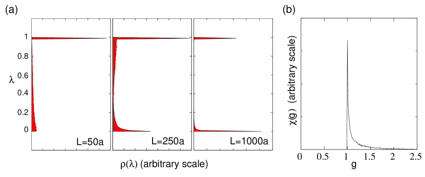
Figure 3: (a) Distribution of the transmission eigenvalues $\lambda$: $\rho(\lambda)$, at $E=0.5$ for $L/a=50,250,1000$, with $d/a=2.0$. $E=0.5$ leads to 3 incident channels. 12,000 samples with different impurity configurations are included in the distribution. (b) Distribution of the dimensionless conductance $g$: $\chi(\lambda)$, at $L/a=1000$ for the same parameter set.

In our model we assume that the impurities are randomly distributed with a density $n_{imp}$, and the potential has a Gaussian form of range $d$

$$V(\bm{r}_{i})=\sum_{\bm{r_{0}}(random)}u\exp\left(-\frac{|\bm{r}_{i}-\bm{r}_{0}|^{2}}{d^{2}}\right)$$ (2)

where the strength $u$ is uniformly distributed within the range $|u|\leq u_{M}$. Here $u_{M}$ satisfies the normalization condition: $u_{M}\sum_{{\bm{r}}_{i}}^{(full\ space)}\exp\left(-{\bm{r}_{i}^{2}}/{d^{2}}\right)/(\sqrt{3}/2)=u_{0}$. The range of the impurity potential is crucial for the transport properties. Since the momentum difference between two valleys is rather large, $\Delta k=k_{+}-k_{-}=4\pi/3a$, only short-range impurities (SRI) with a range smaller than the lattice constant causes inter-valley scattering. Long-range impurties (LRI), in contrast, restrict the scattering processes to intra-valley scattering ando .

We briefly discuss here the relation between valleys in the zigzag ribbons and graphene. The electronic states near the Dirac point can be described by the $\bm{k\cdot p}$ Hamiltonian

$$H_{\bm{k\cdot p}}=\tilde{\gamma}\left[\hat{k}_{x}(\sigma^{x}\otimes\tau^{0})+\hat{k}_{y}(\sigma^{y}\otimes\tau^{z})\right]$$ (3)

acting on the 4-component pseudo-spinor Bloch functions $\Phi=\left[\phi_{\bm{K_{+}}A},\phi_{\bm{K_{+}}B},\phi_{\bm{K_{-}}A},\phi_{\bm{K_{-}}B}\right]$, which characterize the wave functions on the two crystalline sublattices (A and B) for the two Dirac points (valleys) $\bm{K}_{\pm}$. Here, $\tilde{\gamma}$ is the band parameter, $\hat{k}_{x}$($\hat{k}_{y}$) are wavenumber operators, and $\tau^{0}$ is the $2\times 2$ identity matrix. Pauli matrices $\sigma^{x,y,z}$ act on the sublattice space ($A$, $B$), while $\tau^{x,y,z}$ on the valley space ($\bm{K}_{\pm}$). Since the outermost sites along $1^{st}$ ($N^{th}$) zigzag chain are B(A)-sublattice, an imbalance between two sublattices occurs at the zigzag edges leading to the boundary conditions

$$\phi_{\bm{K_{\pm}}A}(\bm{r}_{[0]})=0,\quad\phi_{\bm{K_{\pm}}B}(\bm{r}_{[N+1]})=0,$$ (4)

where $\bm{r}_{[i]}$ stands for the coordinate at $i^{th}$ zigzag chain. It can be shown that the valley near $k=3\pi/2a$ in Fig.1(b) originates from the $\bm{K_{+}}$-point, the other valley at $k=-3\pi/2a$ from $\bm{K_{-}}$-point Phd .

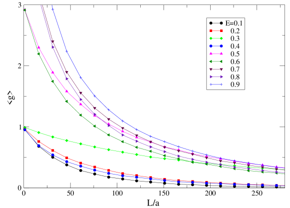
Figure 4: $L$-dependence of the averaged dimensionless conductance for zigzag ribbons with $N=10$, short-ranged impurity potentional ($d/a=0.05$, inter-valley scattering), $u_{0}=1.0$, and $n_{imp.}=0.1$. 5000 samples with different impurity configurations are in the ensemble average.

Ignoring the spins the graphene systems have TRS with respect to the operator $\mathcal{T}$ represented by the complex conjugation $\mathcal{C}$. Pairs of time reversed states are formed across the two-valleys (Dirac points) as expressed in the above pseudo-spinor formulation by $\mathcal{T}=-i(\sigma^{y}\otimes\tau^{0})\mathcal{C}$, where the A-B-sublattices act as pseudospin degrees of freedom. The boundary conditions which treat the two sublattices asymmetrically leading to edge states give rise to a single special mode in each valley. Considering now one of the two valleys separately, say the one around $k=k_{+}$ we see that the TRS is effectively violated in the sense that we find one more left-moving than right-moving mode. If we restrict ourselves to disorder promoting only intra-valley scattering, transport properties would resemble those of a system with a chiral mode which is oppositely oriented for the two valleys. In this sense such a system violates TRS. On the other hand, disorder yielding inter-valley scattering would restore this TRS as both valleys together incorporate a complete set of pairs of time-reversed modes. Thus we expect to see qualitative differences in the properties if the range of the impurity potentials is changed.

In order to demonstrate this we now turn to the discussion of the transport properties. The dimensionless electrical conductance is calculated using the Landauer-Büttiker formulamclbf , $g(E)={\rm Tr}(\bm{t}\bm{t}^{\dagger}),$ where $\bm{t}(E)$ is the transmission matrix through the disordered region. This transmission matrix can be calculated by means of the recursive Green function method green ; prl . We focus first on the case of LRI using a potential with $d/a=1.5$ which is already sufficient to avoid inter-valley scattering. Fig.2 shows the averaged dimensionless conductance as a function of $L$ for different incident energies, averaging over an ensemble of 6000 samples with different impurity configurations for ribbons of the width $N=10$. The potential strength and impurity density are chosen to be $u_{0}=1.0$ and $n_{imp.}=0.1$, respectively. As a typical localization effect we observe that $\langle g\rangle$ gradually decreases with growing length $L$ (Fig.2). Surprisingly, the ribbons remain highly conductive even at the length of $L=1500a$, i.e. more than $350nm$ in the real system. Actually, $\langle g\rangle$ converges to $\langle g\rangle=1$, indicating the presence of a single perfectly conducting channel. It can be seen that $\langle g\rangle(L)$ has an exponential behavior as $\langle g\rangle-1\sim\exp(-L/\xi)$ with $\xi$ as the localization lengthdefxi .

We performed a number of tests to confirm the presence of this perfectly conducting channel. First of all, it exists up to $L=3000a$ for various ribbon widths up to $N=40$ for the potential range ($d/a=1.5$). Moreover it remains for LRI with $d/a=2.0,4.0,6.0,8.0$, and $u_{0}=1.0$, $n_{imp.}=0.1$ and $N=10$. As the effect is connected with the subtle feature of an excess mode in band structure, it is natural that the result can only be valid for sufficiently weak potentials. For potential strengths comparable to the energy scale of the band structure, e.g. the energy difference between the transverse modes, the result should be qualitatively alteredvacancy . Deviations from the limit $\langle g\rangle\to 1$ also occur, if the incident energy lies at a value close to the change between $g=2n-1$ and $g=2n+1$ for the ribbon without disorder. This is for example visible in above calculations for $E=0.4$ where the limiting value $\langle g\rangle<1$ (Fig.2). As a further test we evaluate the distribution of the transmission eigenvalues and dimensionless conductance for fixed wire length. In Fig.3(a), the distribution of the eigenvalues $\lambda$ of the Hermite matrix, $\bm{tt}^{\dagger}$, is depicted for various wire lengths. With growing length $L$ a progressive separation of the transmission eigenvalues emerges with a strong peak close to 0 (localization) and at 1 (perfect conduction channel). The distribution of the conductance $g$ (trace of the transmission matrix ${\rm Tr}(\bm{tt}^{\dagger})$), is depicted in Fig.3(b) for samples in the long-wire limit. Obviously, $g$ only distributes above $g=1$ with a singularity at 1.

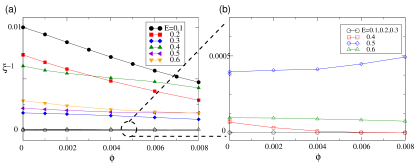
Figure 5: (a) Magnetic field dependence of the inverse localization length $\xi^{-1}$ for various incident energies. The filled symbols indicate data sets of systems with SRI being rather sensitive to magnetic fields, and empty symbols denote data sets for LRI which are almost insensitive to the field. The magnetic flux $\phi$ passing through a single hexagon ring is measured in units of the quantum flux ($\phi_{0}=ch/e$). (b) Enlarged view of (a) of LRI data 5000 samples with different configurations are included in the averages.

Turning to the case of SRI the inter-valley scattering becomes sizable enough to ensure TRS, such that the perfect transport supported by the effective chiral mode in a single valley ceases to exist. SRI causes true back scattering. For a comparison, we show the ribbon length dependence of the averaged conductance in Fig.4. For any incident energy the electrons tend to be localized and the averaged conductance decays exponentially, $\langle g\rangle\sim\exp(-\xi/L)$, without developing a perfect conduction channel.

In order to demonstrate that the qualitative difference between the two regimes, LRI and SRI, is indeed connected with TRS, we study the effect of magnetic field coupling to the electrons through the Peierls phase. For the time reversal symmetric situation resulting from SRI scattering the magnetic field removing TRS should have a stronger effect than for the case of LRI where TRS is broken already at the outset. We use the localization length $\xi$ as an indicator. In Fig.5, the field dependence of the inverse localization length is shown for various incident energies (filled symbols for SRI and empty symbols for LRI). Indeed the localization length displays a stronger field dependence than the LRI. Actually for LRI even a so-called anti-localization behavior with increasing field is visible consistent with recent reports on grapheneantilocalization ; suzuura.prl ; wu . Note that for $E<0.4$ only a single channel is involved in the conductance such that for LRI no localization occurs, i.e. $\xi^{-1}=0$.

The presence of one perfectly conducting channel in disordered quantum wires with symplectic symmetry and an odd number of channels has recently been analyzed using random matrix theory takanesakai . The symplectic symmetry of such systems is based on the skew-symmetry of the reflection matrix, ${}^{t}\bm{r}=-{\bm{r}}$ suzuura . A realization can be found in the disordered metallic carbon nanotubes with LRI. On the other hand, zigzag ribbons without inter-valley scattering are not in the symplectic class, since they break TRS in the special way. The decisive feature for a perfectly conducting channel is the presence of one excess mode in each valley. Note that this is in contrast to graphene for which each mode has a partner mode of reversed velocity in the same valley. For single valley transport the reflection matrix has a non-square form ($N^{(r)}_{c}\times N^{(t)}_{c}$ with $N^{(r)}_{c}=N^{(t)}_{c}+1$, where $N^{(r)}_{c}(N^{(t)}_{c})$ is the number of the reflection (incident) channels). Recently Hirose et. al. pointed out that non-square reflection matrices with unitary symmetry give rise to a perfectly conducting channel ohtsuki .

Eventuelly we can identify the universality classes of zigzag ribbons. For LRI they belong to the unitary class (no TRS), while for SRI with inter-valley scattering they are in the orthogonal class (with overall TRS). This classification is compatible with the behavior in a magnetic field.

Analogous symmetry considerations can be applied to armchair ribbons. In this case the two valleys merge into a single one at $k=0$. TRS is conserved irrespective of the impurity potential range, if there is no magnetic field. Consequently, disordered armchair ribbons belong always to the orthogonal class and do not provide a perfectly conducting channel. In view of the fact that graphene is known to be symplectic (orthogonal) for LRI (SRI) suzuura.prl , it is quite intriguing to realize that the edges influence the universality class, as long as the phase coherence length is larger than the system size of nanographenes.

The unusual energy dispersion due to their edge states gives rise to the unique property of zigzag ribbons. Concerning transport properties for disordered systems the most important consequence is the presence of a perfectly conducting channel. The origin of this effect lies in the single-valley transport which is dominated by a chiral mode. On the other hand, large momentum transfer through impurities with short-range potentials involves both valleys, destroying this effect and leading to usual Anderson localization. The obvious relation of the chiral mode with time reversal symmetry leads to the classification into the unitary and orthogonal class depending on the range of impurity potential. Since the inter-valley scattering is weak in the experiments of graphene, we may assume that these conditions may be realized also for ribbons. Naturally defects in the ribbon edges and vacancies would be rather harmful for the experiment making this type of experiment very challenging prl .

We thank T. Enoki, K. Kusakabe and T. Ohtsuki for stimulating discussions. This work was financially supported by the Swiss Nationalfonds through Centre for Theoretical Studies of ETH Zurich and the NCCR MaNEP, also supported by a Grand-in-Aid for Scientific Research (C) from the Japan Society for the Promotion of Science (No. 16540291). The numerical calculation was performed on the Grid/Cluster Computing System at Hiroshima University.

References

- (1) K. S. Novoselov et. al., Science, 306, 666 (2004); C. Berger et. al., Science, 312, 1191 (2006).
- (2) I. A. Luk’yanchuk, and Y. Kopelevich, Phys. Rev. Lett. 93, 166402 (2004).
- (3) F. D. M. Haldane, Phys. Rev. Lett., 61, 2015 (1988); G. W. Semenoff, ibid., 53, 2449 (1984); V. Gusynin and S. Sharapov, ibid., 95, 146801; A. Castro Net et.al., Phys. Rev. B 73, 205408(2006).
- (4) M. Fujita et. al., J. Phys. Soc. Jpn. 65, 1920 (1996); K. Nakada et. al., Phys. Rev. B 54, 17954 (1996); K. Wakabayashi et. al., Phys. Rev. B 59, 8271 (1999).
- (5) Y. Kobayashi . et. al., Phys. Rev. B 71, 193406 (2005); Y. Niimi et. al., Phys. Rev. B 73, 085421 (2006).
- (6) K. Wakabayashi et. al., Phys. Rev. Lett. 84, 3390 (2000); Phys. Rev. B 64, 125428 (2001).
- (7) K. Wakabayashi, J.Phys.Soc. Jpn.71, 2500 (2002).
- (8) A. Rycerz et. al., cond-mat/0608533.
- (9) Y.-W. Son et. al., Nature 444, 347 (2006).
- (10) M. Büttiker et. al., Phys. Rev. B 31, 6207 (1985).
- (11) T. Ando, Phys. Rev. B 44 8017 (1991).
- (12) N.M.R. Peres, et.al., Phys.Rev.B 73, 195411 (2006).
- (13) T. Ando et. al., J. Phys. Soc. Jpn. 67 1704 (1998); T. Ando et. al., ibid. 67 2857 (1998).
- (14) K. Wakabayashi, Ph.D Thesis, Univ. of Tsukuba, (2000); L. Brey et. al., Phys. Rev. B73, 235411 (2006). Note two virtual zigzag chains on both sides are necessary for the boundary condition on zigzag ribbon of width .
- (15) In this paper, the localization length is evaluated as . Here, () for the system with (without) the perfectly conducting channel.
- (16) E. McCann et. al., Phys. Rev. Lett. 97, 146805 (2005).
- (17) H. Suzuura et. al., Phys. Rev. Lett. 89, 26603 (2002).
- (18) X. Wu et.al., cond-mat/0611339.
- (19) Y. Takane, J. Phys. Soc. Jpn. 73, 9 (2004); H. Sakai and Y. Takane, ibid, 75, 054711 (2005).
- (20) T. Ando et. al., J. Phys. Soc. Jpn. 71, 2754 (2002).
- (21) K. Hirose, T. Ohtsuki, and K. Slevin,unpublished.