Tunneling through magnetic molecules with arbitrary angle
between easy axis and magnetic field

Abstract

Inelastic tunneling through magnetically anisotropic molecules is studied theoretically in the presence of a strong magnetic field. Since the molecular orientation is not well controlled in tunneling experiments, we consider arbitrary angles between easy axis and field. This destroys all conservation laws except that of charge, leading to a rich fine structure in the differential conductance. Besides single molecules we also study monolayers of molecules with either aligned or random easy axes. We show that detailed information on the molecular transitions and orientations can be obtained from the differential conductance for varying magnetic field. For random easy axes, averaging over orientations leads to van Hove singularities in the differential conductance. Rate equations in the sequential-tunneling approximation are employed. An efficient approximation for their solution for complex molecules is presented. The results are applied to $\mathrm{Mn}_{12}$-based magnetic molecules.

I Introduction

Electronic transport through single magnetic molecules has recently attracted a lot of interest,PPG02 ; LSB02 ; PaF05 ; ElT05 ; HGF06 ; RWH06 ; RWS06 ; TiE06 ; ElT06 ; JGB06 ; LeM06 ; DGR06 ; MiB06 ; GoL06 ; ElT07 partly motivated by the hope for applications in molecular electronics,Joachim ; Har02 ; XuR06 in particular for memory devices and quantum computation. On the other hand, the systems also show fascinating properties of fundamental interest. Among effects observed or predicted for transport through magnetic molecules are the Kondo effect,PPG02 ; LSB02 negative differential conductance,HGF06 ; RWS06 also at room temperature,ElT06 large spin accumulation in the leads controlled by the initial spin state of the molecule,TiE06 and large current-induced magnetization changes in monolayers.ElT07

Molecules with magnetic anisotropy are observedHGF06 ; JGB06 or predictedRWH06 ; RWS06 ; TiE06 ; ElT06 ; ElT07 to show particularly rich physics. Magnetic molecules based on a $\mathrm{Mn}_{12}\mathrm{O}_{12}$ core with organic ligands (henceforce $\mathrm{Mn}_{12}$) have a large spin $S=10$ in the neutral state and strong easy-axis anisotropy.PaP04 ; HGF06 ; JGB06 ; RWH06 ; RWS06 The anisotropy leads to an energy barrier between states with large positive or negative spin components along the easy (z) axis. $\mathrm{Mn}_{12}$ has been studied intensively with regard to quantum tunneling through this barrier.FST96 ; MSS03 Recently, charge transport through $\mathrm{Mn}_{12}$ has been studied.HGF06 ; JGB06 ; RWH06 ; RWS06

Romeike et al.RWH06 ; RWS06 investigate the effect of quantum tunneling on transport through $\mathrm{Mn}_{12}$. They consider small non-uniaxial second-order anisotropy terms $(S^{x})^{2}-(S^{y})^{2}=(S^{+})^{2}/2+(S^{-})^{2}/2$ and higher-order anisotropies, see also Ref. HGF06, . The non-uniaxial terms are not present for the isolated $\mathrm{Mn}_{12}$ moleculePaP04 but are due to the lowering of symmetry by the leads. These non-uniaxial terms destroy the conservation of the $z$ component of the molecular spin, $S_{\mathrm{tot}}^{z}$. The molecular energy eigenstates are then not simultaneous eigenstates of $S_{\mathrm{tot}}^{z}$. Since the non-uniaxial perturbation is small, one can still work in a basis of $S_{\mathrm{tot}}^{z}$ eigenstates, but incurs weak tunneling transitions between them, which are at the basis of Refs. RWH06, ; RWS06, . Importantly for the present discussion, they also study $\mathrm{Mn}_{12}$ in a magnetic field aligned with the easy axis.

The present paper starts from the realization that there is a much stronger symmetry-breaking effect if an external magnetic field is applied. In present-day break-junction and electromigration experiments, the orientation of the molecule relative to the laboratory frame is not well-controlled. However, if the angle $\theta$ between the easy axis and the magnetic field is not small and the Zeeman and anisotropy energies are comparable—a case that can be realized for $\mathrm{Mn}_{12}$—there is no small parameter. The molecular eigenstates are not approximate eigenstates of the spin component along any axis. This is the situation studied in the present paper.

In Sec. II the model Hamiltonian is introduced and the calculation of the differential conductance is discussed. We employ a density-matrix formalism, which allows to treat the strong electronic interaction on the molecule exactly and is not restricted to low bias voltages, but treats the tunneling between molecule and leads as a weak perturbation.Blu81 ; ScS94 ; KSS95 ; TuM02 ; BrF04 ; Mitra ; KOO04 ; ElT05 ; KoO05 ; RWS06 ; TiE06 ; ElT06 ; ElT07 An approximation scheme for solving the resulting rate equations is introduced, which works excellently at low temperatures and leads to a large acceleration of the numerics. Results are presented and discussed in Sec. III, starting with Coulomb-diamond plots of differential conductance $g$ vs. gate and bias voltages. Then $g$ is shown for varying magnetic field. These results are also relevant for situations without a gate such as the STM geometry or monolayers of molecules with parallel easy axes. Finally, the differential conductance for monolayers of molecules with random easy-axis orientations is calculated. The main results are summarized in Sec. IV.

II Model and theory

A magnetic molecule coupled to two conducting leads L (left) and R (right) is described by the Hamiltonian $H=H_{\mathrm{mol}}+H_{\mathrm{L}}+H_{\mathrm{R}}+H_{\mathrm{hyb}}$. Here, $H_{\mathrm{mol}}$ is the Hamiltonian of the isolated molecule,

$$H_{\mathrm{mol}}=(\epsilon_{0}-eV_{g})\sum_{\sigma}c_{\sigma}^{\dagger}c_{\sigma}+Uc_{\uparrow}^{\dagger}c_{\uparrow}c_{\downarrow}^{\dagger}c_{\downarrow}$$ (1)

$${}-\Big{(}K_{2}+\kappa\sum_{\sigma}c_{\sigma}^{\dagger}c_{\sigma}\Big{)}(S^{z})^{2}-\mathbf{H}\cdot(\mathbf{s}+\mathbf{S})-J\mathbf{s}\cdot\mathbf{S},\quad$$

where $c_{\sigma}^{\dagger}$ creates an electron in the lowest unoccupied molecular orbital (LUMO), $\mathbf{s}\equiv\sum_{\sigma\sigma^{\prime}}c_{\sigma}^{\dagger}\,(\mbox{\boldmath$\sigma$}_{\sigma\sigma^{\prime}}/2)\,c_{\sigma^{\prime}}$ is the spin operator of electrons in the LUMO, and $\mathbf{S}$ is the operator of the local spin. We also define the total spin $\mathbf{S}_{\mathrm{tot}}\equiv\mathbf{s}+\mathbf{S}$. $\epsilon_{0}$ is the onsite energy of electrons in the LUMO, which can be shifted by applying a gate voltage $V_{g}$, $U$ is the repulsion between two electrons in the LUMO, and $J$ is the exchange interaction between the electron spin and the local spin. A dependence of the anisotropy energy $K_{2}+\kappa n$ on the electron number $n$ is taken into account.PaP04

The g-factors for the local and electron spins are assumed to be equal and are absorbed into the magnetic field $\mathbf{H}$, together with the Bohr magneton $\mu_{B}$. We choose the easy axis of the molecule as the z axis in spin space. Due to the rotational symmetry of $H_{\mathrm{mol}}$, the magnetic field can be assumed to lie in the xz plane. We neglect the small non-uniaxial anisotropy due to the symmetry breaking by the leads and small higher-order anisotropies in order to concentrate on the large effect due to the interplay of anisotropy and Zeeman terms.

The Hamiltonian explicitly takes the electron in the LUMO into account, which is non-degenerate for $\mathrm{Mn}_{12}$.PaP04 Since the next higher energy orbital (LUMO$+1$) lies about $8\,\mathrm{meV}$ above the LUMO,PaP04 this and higher orbitals are expected to affect the results only weakly at the low bias voltages discussed here. Excitations to one of the higher-energy orbitals are presumably responsible for the $14\,\mathrm{mV}$ peak observed in Ref. HGF06, .

We assume that the molecule is symmetrically coupled to the leads $\alpha=\mathrm{L},\mathrm{R}$ by hybridization terms $H_{\mathrm{hyb}}=\sum_{\alpha\mathbf{k}\sigma}(t\,a^{\dagger}_{\alpha\mathbf{k}\sigma}c_{\sigma}+\mathrm{h.c.})$, where $a^{\dagger}_{\alpha\mathbf{k}\sigma}$ creates an electron in lead $\alpha$. The leads are described by non-interacting electrons, $H_{\alpha}=\sum_{\mathbf{k}\sigma}\epsilon_{\alpha\mathbf{k}\sigma}\,a^{\dagger}_{\alpha\mathbf{k}\sigma}a_{\alpha\mathbf{k}\sigma}$.ElT05 ; TiE06 ; ElT06 ; ElT07

There are important consequences of the presence of the transverse field $H_{x}$. Since this term does not commute with the anisotropy term, $S_{\mathrm{tot}}^{z}$ is not conserved and the molecular eigenstates (of $H_{\mathrm{mol}}$) are not simultaneous eigenstates of $S_{\mathrm{tot}}^{z}$. On the other hand, if the magnetic field is aligned with the easy axis,TiE06 ; ElT06 ; ElT07 the eigenvalue $m$ of $S_{\mathrm{tot}}^{z}$ is a good quantum number and electron tunneling is governed by selection rules $\Delta m=\pm 1/2$ for sequential tunneling. These selection rules do not apply to our case. The only selection rule still valid stems from the conservation of charge and states that the electron number changes by $\pm 1$ for sequential tunneling. Apart from this, all transitions are allowed. For local spin quantum number $S$, there are $2S+1$ molecular states with $n=0$ electrons in the LUMO and $2(2S+1)$ states with $n=1$ electrons. Thus there are $2(2S+1)^{2}$ transitions between states with $n=0$ and $n=1$, leading to a much more complex differential conductance $g$ than for the previous case.TiE06 ; ElT06 ; ElT07

The same model can also be used to describe a monolayer of magnetic molecules sandwiched between conducting electrodes, if the tunneling rate between electrodes and molecule is sufficiently small to justify the perturbative treatment. This can in principle be achieved by spacer groups in the molecules or by ultrathin oxide layers. If the interactions between the molecules can be neglected, they conduct electrons in parallel, and the differential conductance per molecule is just the ensemble average we are calculating in any case. For a single molecule, we have to re-interpret the ensemble average as a time average over time scales long compared to the characteristic tunneling time.

These remarks only hold for identical molecules, which requires all molecules to have their easy axes aligned in parallel. This is a reasonable assumption for molecules that are deposited or assembled on the substrate with a preferred orientation.ElT07 This has been demonstrated for mixed $\mathrm{Mn}_{12}$ complexes containing different ligands.FCH05 For molecules of approximately spherical shape one rather expects the orientation of the easy axis to be random. To study this case, we average the differential conductance over all possible orientations. Conversely, measurements of the differential conductance can be employed to determine the degree of alignment.

The absence of constants of motion other than particle number requires to diagonalize $H_{\mathrm{mol}}$ numerically. The eigenstates typically contain contributions from all spin $S_{\mathrm{tot}}^{z}$ eigenstates. The hybridization $H_{\mathrm{hyb}}$ is treated as a perturbation, following Refs. Blu81, ; Mitra, ; KOO04, ; ElT05, . This leads to a master equation for the reduced density matrix $\rho_{\mathrm{mol}}$ in the Fock space of $H_{\mathrm{mol}}$.

The master equation still contains off-diagonal components of $\rho_{\mathrm{mol}}$, corresponding to superpositions of molecular eigenstates. However, in the presence of non-commuting Zeeman and anisotropy terms in the Hamiltonian, any two states differ in the spin expectation value $\langle\mathbf{S}_{\mathrm{tot}}\rangle$, which leads to different long-range magnetic fields. Thus the unavoidable interaction between the molecule and many degrees of freedom in the environment (e.g., electron spins) should impart superselection rulesZur82 ensuring that the dephasing of superpositions is rapid. For states with different charge, the Coulomb field also leads to strong superselection rules.Zur82

It is thus sufficient to consider the rate equations for the probabilities $P_{m}\equiv(\rho_{\mathrm{mol}})_{mm}$ of molecular states $|m\rangle$,

$$\dot{P}_{m}=\sum_{n\neq m}(R_{n\to m}P_{n}-R_{m\to n}P_{m}).$$ (2)

The stationary-state probabilities $P^{(0)}_{m}$ are determined by $\dot{P}^{(0)}_{m}=0$. The transition rates $R_{m\to n}$ are written as a sum over leads and spin directions, $R_{m\to n}=\sum_{\sigma\alpha}R^{\sigma\alpha}_{m\to n}$, with

$$R^{\sigma\alpha}_{m\to n} = \frac{1}{\tau_{0}}\big{[}f(\epsilon_{n}-\epsilon_{m}+es_{\alpha}V/2)\,|C_{mn}^{\sigma}|^{2}$$ (3)

$${}+f(\epsilon_{n}-\epsilon_{m}-es_{\alpha}V/2)\,|C_{nm}^{\sigma}|^{2}\big{]},$$

where $s_{\mathrm{L}}=1$, $s_{\mathrm{R}}=-1$, $1/\tau_{0}\equiv 2\pi\,|t|^{2}\,Dv_{\mathrm{uc}}/\hbar$ is the typical transition rate in terms of the density of states $D$ (for one spin direction) of the leads and their unit-cell volume $v_{\mathrm{uc}}$, $V$ is the bias voltage, $\epsilon_{m}$ is the energy of state $|m\rangle$, $f(x)$ is the Fermi function, and $C_{mn}^{\sigma}\equiv\langle m|c_{\sigma}|n\rangle$ are transition matrix elements. The current $I_{\alpha}$ through lead $\alpha$ can be expressed in terms of the rates and probabilities,

$$I_{\alpha}=-e\,s_{\alpha}\sum_{mn\sigma}(n_{m}-n_{n})\,R^{\sigma\alpha}_{n\to m}\,P_{n},$$ (4)

where $n_{m}$ is the number of electrons for state $|m\rangle$. We are interested in the stationary state for which the current through both leads is equal. Therefore, we drop the subscript $\alpha$ and insert the stationary-state probabilities $P^{(0)}_{n}$. We will mainly analyze the differential conductance $g\equiv dI/dV$.

In principle, the solution of the equations $\dot{P}^{(0)}_{m}=0$ is simple: The probabilities $P^{(0)}_{m}$ form an eigenvector of a matrix $A$ to zero eigenvalue, where $A_{mn}=R_{n\to m}$ for $m\neq n$ and $A_{mm}=-\sum_{p\neq m}R_{m\to p}$. However, numerical diagonalization often fails because the components of $A$, the rates, vary over many orders of magnitude due to the Fermi factors in Eq. (3). The ratio of very small rates can have a large effect on the probabilities, in particular for anisotropic magnetic molecules.TiE06 ; ElT06 Consequently, truncation errors in the very small rates can lead to large errors in the probabilities.

An approach that avoids this problem would be highly welcome. One such approach relies on the enumeration of all tree graphs on the network of molecular states connected by allowed transitions.Hil66 ; Sch76 ; ZiS06 However, this approach is not feasible for large molecular Fock spaces, since it requires summation over of the order of $N^{N-2}$ tree graphsZiS06 for each $P^{(0)}_{m}$, where $N$ is the dimension of the space.

The solution at $T=0$ is simpler and less susceptible to truncation errors because the Fermi factors are all either zero or unity. Thus there are no exponentially small rates, unless some matrix elements $C^{\sigma}_{mn}$ are exponentially small. This is not the case for generic angles $\theta$ between magnetic field and easy axis. We here employ an approximation scheme to find the $P^{(0)}_{m}$ and the current $I$. The scheme relies on solving the rate equations and calculating the current exactly at $T=0$ and introducing broadening of the steps in $P^{(0)}_{m}$ and $I$ to take finite temperatures into account. Details are presented in App. A. The approximation is excellent at sufficiently low temperatures. It speeds up the calculation of $g$ for $500\times 500$ values of $V_{g}$ and $V$ and spin $S=2$ by a factor of about 350.

III Results and discussion

In the following, we discuss results for molecules with local spin $S=2$ and $S=10$. The smaller spin allows to exhibit the physics more clearly, since the number of relevant transitions is smaller. As noted above, there are $2(2S+1)^{2}$ transitions between states with zero and one electron, which gives $50$ for $S=2$ and $882$ for $S=10$. These are the maximum possible numbers of differential-conductance peaks. For $S=2$, we choose parameter values that allow to discuss the effects of interest but do not correspond to a specific molecule.

For $S=10$ we use realistic parameters for $\mathrm{Mn}_{12}$ calculated by Park and PedersonPaP04 employing density functional theory in the generalized-gradient approximation. We take $K_{2}=0.0465\,\mathrm{meV}$, $\kappa=-0.00862\,\mathrm{meV}$ (taken from results for potassium doping), and $J=3.92\,\mathrm{meV}$ (from the energy difference of states with $m=21/2$ and $m=19/2$, respectively, where $m$ is the quantum number of $S^{z}_{\mathrm{tot}}$). $K_{2}$ is close to the experimental value $K_{2}=0.056\,\mathrm{meV}$ from Ref. HGF06, .

The onside energy $\epsilon_{0}$ cannot be inferred from Ref. PaP04, . The LUMO–HOMO gap is $E_{g}=438\,\mathrm{meV}$.PaP04 Since $\mathrm{Mn}_{12}$ is found to be more easily negatively doped, we can assume $\epsilon_{0}$ to lie closer to the LUMO. In experiments with a gate, the onsite energy is shifted to $\epsilon_{0}-eV_{g}$ in any case. For single $\mathrm{Mn}_{12}$ molecules, we will mainly consider the parameter region close to the crossing point where states with $n=0$ and $n=1$ become degenerate. Finally, we choose a very large value for $U$ so that double occupation of the LUMO is forbidden.

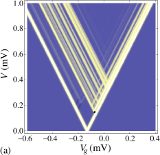
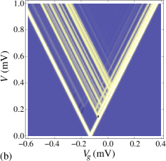
Figure 1: (Color online) Differential conductance $g=dI/dV$ as a function of gate voltage $V_{g}$ and bias voltage $V$. Bright (dark) colors denote $g>0$ ($g<0$). The parameters are $S=2$, $\epsilon_{0}=0$, $U=10$, $H_{x}=H_{z}=0.05$, $K_{2}=0.04$, $\kappa=0$, $J=0.1$, and $T=0.002$ (all energies in meV). (a) Results obtained by exact solution of the rate equations. (b) Results of the approximation of App. A.

III.1 Gate-voltage scans

We start by presenting a typical differential-conductance plot as a function of gate voltage $V_{g}$ and bias voltage $V$ for spin $S=2$ in Fig. 1. The magnetic field is applied at an angle $\theta=45^{\circ}$ relative to the easy axis. The comparison of the exact solution of the stationary-state rate equations with the approximation of App. A shows excellent agreement.

The blue (medium gray) regions to the left and right of the crossing point in Fig. 1 correspond to Coulomb blockade (CB) with small current and electron numbers $n=0$ and $n=1$, respectively. The plot would be mirror symmetric for $V<0$. The CB regions are delimited by strong peaks at the CB threshold, where the current increases rapidly to a large value of order $e/\tau_{0}$. In the absence of internal degrees of freedom of the molecule this would be the only structure in the plots. However, the interaction of the tunneling electron with the local spin leads to inelastic tunneling processes, which cause the peaks at the CB threshold to split.

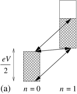
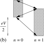
Figure 2: Sketch of molecular energy multiplets (a) to the left of the crossing point in Fig. 1 (ground state with $n=0$ electrons) and (b) to the right of the crossing point (ground state with $n=1$). A few representative transitions are shown as double-headed arrows. Generically, all transitions between states with $n=0$ and $n=1$ have nonzero matrix elements. The bias voltage $V$ is at the CB threshold in both cases. States that become populated at the CB threshold at $T=0$ are cross-hatched. In (a) some states with $n=1$ do not become active at the CB threshold (white rectangle).

The resulting fine structure is much more complex than for magnetic molecules without anisotropyElT05 or in the absence of a strong magnetic field,TiE06 ; ElT07 since there are many more allowed transitions in the present model due to non-commuting Zeeman and anisotropy terms. Each peak in $g$ corresponds to one or more allowed transitions becoming energetically possible. The peak at the CB threshold is much stronger (the current step is much higher) than the peaks at higher bias voltage, since many additional transitions become available at the CB threshold, as illustrated by Fig. 2.

Figure 1 also shows strong asymmetry between the fine structure on both sides of the crossing point. This is due to the multiplet of states with $n=1$ being broader in energy than the one with $n=0$. Figure 2 shows that for a ground state with $n=0$, not all states with $n=1$ become active (obtain nonzero probability at $T=0$) at the CB threshold, whereas for a ground state with $n=1$, all state with $n=0$ become active. Thus for the first case, to the left of the crossing point, there are more $g$ peaks where additional states with $n=1$ become active.

Why then are there any additional lines to the right of the crossing point? Here, all $n=0$ states become active at the CB threshold. However, the probabilities and the current show steps when additional transitions become energetically possible even if the final state of these transitions was already active. This mechanism leads to $g$ peaks on both sides.

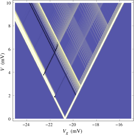
Figure 3: (Color online) Differential conductance $g$ as a function of gate voltage $V_{g}$ and bias voltage $V$ for $\mathrm{Mn}_{12}$ in a magnetic field perpendicular to the easy axis. Bright (dark) colors denote $g>0$ ($g<0$). The parameters are $S=10$, $\epsilon=0$, $U=10000$, $H_{x}=2.32$ (corresponding to $20\,\mathrm{T}$), $H_{z}=0$, $K_{2}=0.0465$, $\kappa=-0.00862$, $J=3.92$, and $T=0.00863$ ($0.1\,\mathrm{K}$), where all energies are in meV. The approximation of App. A has been used.

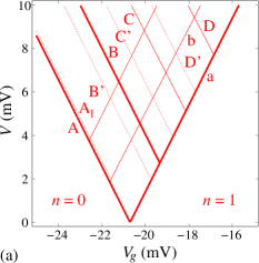
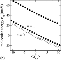
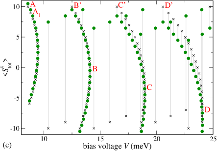
Figure 4: (Color online) (a) $g$ peaks corresponding to special transitions in Fig. 3, see text. (b) Molecular energy levels vs. spin expectation value $\langle S_{\mathrm{tot}}^{x}\rangle$, for $\epsilon_{0}-eV_{g}=25\,\mathrm{mV}$. Open (solid) circles correspond to states with $n=0$ ($n=1$) electrons in the LUMO. (c) Spin expectation values $\langle S_{\mathrm{tot}}^{x}\rangle$ of initial (crosses) and final (circles) states vs. bias voltage for the lowest-lying $g$ peaks, for $\epsilon_{0}-eV_{g}=25\,\mathrm{meV}$. Only transitions starting from states with $n=0$ are shown. Special transitions are labeled as in (a).

Next, we consider parameters for $\mathrm{Mn}_{12}$. Figure 3 shows $g(V_{g},V)$ for a strong transverse field ($H_{z}=0$) close to the crossing point between CB with $n=0$ and $n=1$. Note that $\epsilon_{0}$ has been set to zero, the zero of $V_{g}$ is thus arbitrary. Figure 4(a) shows a sketch of special features in Fig. 3.

The plots show two clear energy scales. For the strong magnetic field ($20\,\mathrm{T}$) in Fig. 3, the Zeeman energy dominates over the anisotropy energy. The molecular states are nearly eigenstates of $S_{\mathrm{tot}}^{x}$. In the following we use Fig. 3 as an example for the analysis of differential-conductance plots for complex molecules. We concentate on the case when the ground state has $n=0$ electrons, to the left of the crossing point.

To facilitate the analysis, Fig. 4(b) shows the energy of low-lying molecular states vs. the expectation value $\langle S_{\mathrm{tot}}^{x}\rangle$, which is nearly a good quantum number. Figure 4(c) shows, for each differential-conductance peak (current step) occuring at low bias voltage, the spin expectation value $\langle S_{\mathrm{tot}}^{x}\rangle$ for the initial (cross) and final (circle) state vs. the bias voltage. Only transitions starting from states with $n=0$ are included, these have negative slope in Fig. 3. Several transitions are marked with the same letters as in Fig. 4(a). These plots assume $\epsilon_{0}-eV_{g}=25\,\mathrm{meV}$ (the left edge of Fig. 3), but the conclusions hold in general far left of the crossing point.

The CB threshold corresponds to transition A in Figs. 4(a) and (c). Since all matrix elements between states with $n=0$ and $n=1$ are nonzero, nearly all states belonging to the low-energy ladder in Fig. 4(b) assume nonzero probabilities even at $T=0$ as soon as transition A becomes energetically possible.footnote.highmulti As noted above, this makes the threshold peak anomalously strong.

The second strong line corresponds to transition B. Without anisotropy, A and B would be the only visible transitions from $n=0$ to $n=1$, since transition A (B) would correspond to a change in $\langle S_{\mathrm{tot}}^{x}\rangle$ by $+1/2$ ($-1/2$) and these would be the only allowed changes. Also, the ladders of $n=0$ and $n=1$ levels would be exactly parallel so that all allowed transitions would have one of these two energies. In our case, the anisotropy leads to additional allowed transitions C, D,…etc. corresponding to changes of $\langle S_{\mathrm{tot}}^{x}\rangle$ by approximately $-3/2,-5/2,\ldots$, respectively.

The peaks show additional fine structure with a smaller energy scale coming from the anisotropy. The CB-threshold peak is accompanied by additional peaks at slightly higher bias. The first visible one corresponds to transition $\mathrm{A}_{1}$ in Fig. 4(c). Peaks B, C, D are accompanied by series of peaks at lower bias, reaching down to B’, C’, D’. These peaks correspond to arc-shaped series of transitions with approximately the same change in $\langle S_{\mathrm{tot}}^{x}\rangle$. There are a few additional transitions with large changes in $\langle S_{\mathrm{tot}}^{x}\rangle$ in Fig. 4(c). These are not visible in Fig. 3 due to very small transition matrix elements.

Several peaks, in particular B’, show negative differential conductance (NDC). The origin is the following:TiE06 The current equals the charge $e$ times a typical tunneling rate. This tunneling rate is a weighted average over the rates of energetically possible transitions. But transition B’ has a small rate due to small $C^{\sigma}_{mn}$, as numerical calculation shows. Therefore, the typical tunneling rate and the current decrease at B’.

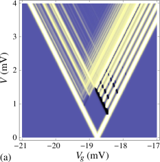
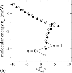
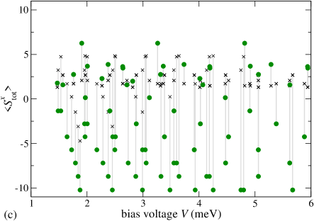
Figure 5: (Color online) (a) Differential conductance $g$ as in Fig. 3 except for a smaller magnetic field, $H_{x}=0.116\,\mathrm{meV}$ ($1\,\mathrm{T}$). The approximation of App. A has been used. (b) Molecular energy levels vs. spin expectation value $\langle S_{\mathrm{tot}}^{x}\rangle$, for $\epsilon_{0}-eV_{g}=19.5\,\mathrm{mV}$. Open (solid) circles correspond to states with $n=0$ ($n=1$). (c) Spin expectation values $\langle S_{\mathrm{tot}}^{x}\rangle$ of initial (crosses) and final (circles) states vs. bias voltage for the lowest-lying $g$ peaks, for $\epsilon_{0}-eV_{g}=19.5\,\mathrm{meV}$. Only transitions starting from states with $n=0$ are shown.

For comparison, Fig. 5(a) shows the differential conductance for a smaller transverse field leading to comparable Zeeman and anisotropy energies. In this case, the molecular states are no longer approximate eigenstates of $S_{\mathrm{tot}}^{x}$, cf. Fig. 5(b). This leads to a more complicated fine structure. It is still possible to attribute peaks to specific molecular transitions, as comparison with the map of transitions in Fig. 5(c) shows, but the spectrum and the transition energies look more random.

Note that the fine structure splitting is now broader where the ground state has $n=1$ electrons, opposite to the $S=2$ molecule, cf. Fig. 1. This stems from the smaller anisotropy $K_{2}+\kappa<K_{2}$ in the $n=1$ case, which makes the multiplet of accessible $n=1$ states narrower in energy than the $n=0$ multiplet, as seen in Fig. 5(b).footnote.Jstates

III.2 Magnetic-field scans

Our main topic is the interplay of magnetic field and anisotropy. Since the Zeeman and anisotropy terms in the Hamiltonian do not commute and are assumed to be comparable in magnitude, we expect the differential conductance $g$ to depend significantly on the field. The natural way to study this is to plot $g$ as a function of quantities characterizing the magnetic field and possibly of bias voltage. Such magnetic-field scans could, in principle, also be done experimentally.

Since a gate electrode is not required, magnetic-field scans could also be taken for monolayers of molecules sandwiched between conducting electrodesElT07 or with an STM for single molecules or monolayers. For the theory to be applicable, the tunneling between molecule and electrodes must be made sufficiently weak to justify the sequential-tunneling approximation, e.g., by molecular spacer groups or a thin oxide layer.QNH04 The present subsection thus applies to single molecules and to monolayers of molecules with aligned easy axes.

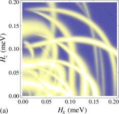
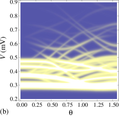
Figure 6: (Color online) (a) Differential conductance $g$ as a function of the magnetic field components $H_{x}$ (perpendicular to easy axis) and $H_{z}$ (parallel to easy axis). Bright (dark) colors denote $g>0$ ($g<0$). The parameters are $S=2$, $\epsilon_{0}-eV_{g}=0.2$, $U=10$, $K_{2}=0.04$, $\kappa=0$, $J=0.1$, $T=0.002$ (all energies in meV), and $V=0.8\,\mathrm{mV}$. The rate equations have been solved exactly. (b) $g$ as a function of the angle $\theta$ between magnetic field and easy axis and bias voltage $V$ for the $S=2$ model in a magnetic field $|\mathbf{H}|=0.1\,\mathrm{meV}$. The other parameters are as in Fig. 1. The approximation of App. A has been used.

Figure 6(a) shows $g$ as a function of magnetic-field components $H_{x}$ and $H_{z}$ for the case of spin $S=2$ for fixed gate and bias voltages, $\epsilon_{0}-eV_{g}=0.2\,\mathrm{meV}$ and $V=0.8\,\mathrm{mV}$, respectively. This plot shows $g$ if one fixes $V_{g}$ and $V$ in Fig. 1 and varies the magnetic field. A peak in $g$ appears whenever an allowed and energetically possible transition crosses the energy $eV/2$. Figure 6(a) can be extended to all values of $\mathbf{H}$ using the rotational symmetry of $g$ around the z (easy) axis and the reflection symmetry in the xy plane.

Clearly, the symmetry of $g(\mathbf{H})$ allows to determine the orientation of the molecule(s) from a transport measurement in a magnetic field. This is useful since the orientation is typically poorly controlled and is not easy to determine in break-junction and electromigration experiments.

The structure in Fig. 6(a) is richer than that in Fig. 1: Curves of large $g$ are not straight and they vary in intensity (height of the current step) and can even vanish. They are not straight because they correspond to differences of two eigenenergies of $H_{\mathrm{mol}}$ and the eigenenergies are complicated functions of $\mathbf{H}$, since the Zeeman term does not commute with the anisotropy term. Nevertheless it is remarkable that the relatively simple model with spin $S=2$ generates this complex structure.

The $g$ peaks in Fig. 6(a) change in intensity with magnetic field since the transition matrix elements $C^{\sigma}_{mn}$ change. In the limiting case of $H_{x}=0$, i.e., field parallel to the easy axis, the Zeeman and anisotropy terms do commute. In this case $S_{\mathrm{tot}}^{z}$ is conserved, and transitions changing $S_{\mathrm{tot}}^{z}$ by values other than $\pm 1/2$ are forbidden. Curves belonging to these transitions vanish for $H_{x}\to 0$.

Figure 6(b) shows $g$ as a function of bias voltage $V$ and the angle $\theta$ between field and easy axis. Note again that several peaks vanish for $\theta\to 0$, where the transitions become forbidden. The plot shows that the strong peak at the CB threshold also depends on the magnetic-field direction. It is thus possible to switch the molecule between CB, with very small current due to cotunneling,ElT07 and a state with large current, leading to a large and anisotropic magnetoresistance at low temperatures.

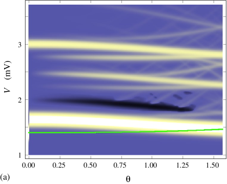
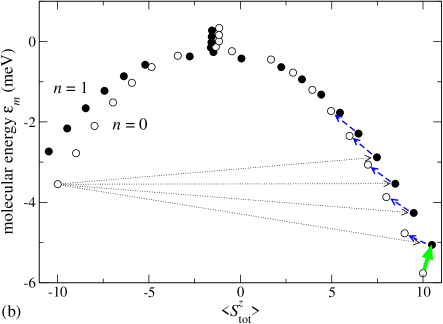
Figure 7: (Color online) (a) Differential conductance $g$ as a function of the angle $\theta$ between magnetic field and easy axis and bias voltage $V$ for $\mathrm{Mn}_{12}$ in a magnetic field $|\mathbf{H}|=0.116\,\mathrm{meV}$ ($1\,\mathrm{T}$) at temperature $T=0.00863\,\mathrm{meV}$ ($0.1\,\mathrm{K}$). The other parameters are as in Figs. 3 and 5. The approximation of App. A has been used. The solid (green) curve denotes the CB threshold, which is invisible in $g$ for $\theta>0$ due to the presence of a blocking state. (b) Molecular energy levels vs. spin expectation value $\langle S_{\mathrm{tot}}^{z}\rangle$ for $\theta=0.3$. Open (solid) circles correspond to states with $n=0$ ($n=1$) electrons. The blocking state has $n=0$ and $\langle S^{z}_{\mathrm{tot}}\rangle\approx-10$. Transitions discussed in the text are marked by arrows (most allowed transitions are not marked).

Figure 7(a) shows $g(\theta,V)$ for $\mathrm{Mn}_{12}$. On first glance, similar features as in Fig. 6(b) are seen. However, an important new effect is at work here: Analysis of the $\theta=0$ case shows that the CB threshold for $\theta=0$ corresponds to the transition from $m=10$ to $m=21/2$, where now $m$ is the quantum number of $S^{z}_{\mathrm{tot}}$. The corresponding bias voltage is $V_{\mathrm{CB}}=1.41\,\mathrm{mV}$. However, Fig. 7(a) does not show a strong peak at this bias for small $\theta>0$. Rather, the threshold appears to be at about $V=1.64\,\mathrm{mV}$.

The molecular levels shown in Fig. 7(b) help to understand this situation: the first possible transition at $T=0$ is the one from $\langle S^{z}_{\mathrm{tot}}\rangle\approx 10$ to $\langle S^{z}_{\mathrm{tot}}\rangle\approx 21/2$, denoted by a solid curve in Fig. 7(a) and a solid arrow in (b). For $\theta=0$ this leads to a large current associated with repeated transitions between these two states, which are the only allowed ones until the transition to $\langle S^{z}_{\mathrm{tot}}\rangle\approx 19/2$ becomes possible at higher bias. However, for $\theta>0$ there are nonzero matrix elements for transitions that decrease $\langle S^{z}_{\mathrm{tot}}\rangle$ by about $3/2$ (dashed arrows). Consequently, the molecule can reach the states with $\langle S^{z}_{\mathrm{tot}}\rangle\approx 0$. From there, it can relax to states with negative $\langle S^{z}_{\mathrm{tot}}\rangle$ through transitions with large rates, in particular to the state with $\langle S^{z}_{\mathrm{tot}}\rangle\approx-10$. But this is essentially a blocking state, since the transitions to $\langle S^{z}_{\mathrm{tot}}\rangle\approx-21/2$ and $-19/2$ are energetically impossible and the only transitions that are energetically possible correspond to very large changes of $\langle S^{z}_{\mathrm{tot}}\rangle$ (dotted arrows) and have extremely small matrix elements. This is thus an example of spin blockade. Note that cotunneling transitions out of the blocking state to $\langle S^{z}_{\mathrm{tot}}\rangle\approx-9$ are possible, since the full potential difference $eV$ is available for excitations. This leads to a very small current dominated by cotunneling, which would still be invisible in Fig. 7(a).

To summarize, while transitions from positive to negative $\langle S^{z}_{\mathrm{tot}}\rangle$ happen only with a small rate, transitions in the opposite direction occur with a still much smaller rate. Consequently, the molecule is nearly always in the $\langle S^{z}_{\mathrm{tot}}\rangle\approx-10$ state and the current is extremely small.footnote.dyna Thus there is no visible differential-conductance peak at the CB threshold.

We conclude with two remarks: (i) The discontinuity of $g$ at $\theta=0$ is irrelevant in practice, since it is impossible to perfectly align the molecular easy axis with the field. (ii) Figure 7(a) shows that the CB threshold coincides with the strong $g$ peak for $\theta=\pi/2$. In this case, Fig. 7(b) would be symmetric under spin inversion so that the states with $\langle S^{z}_{\mathrm{tot}}\rangle\approx\pm 10$ become degenerate ground states and there is no blocking state. This case was studied in Figs. 3 and 4.

III.3 Orientational disorder

So far we have considered tunneling through single molecules or through monolayers of molecules with parallel easy axes.FCH05 Depending on the ligands, $\mathrm{Mn}_{12}$ can be nearly spherical. In that case the distribution of orientations in a monolayer will be closer to random.

To describe tunneling through a monolayer of randomly oriented magnetic molecules, we have to average the current and differential conductance over all orientations. Equivalently, we here average over all magnetic-field directions relative to the molecular easy axis. One might expect that this smears out most of the fine structure. As we shall see, this is not the case. The averaged differential conductance $\overline{g}$ as a function of bias voltage $V$ is rather complex due to van Hove singularities coming from extrema and crossings in the transition energies as functions of magnetic field direction.

The angle-averaged differential conductance per molecule is $\overline{g}=(1/4\pi)\int d\theta\,d\phi\,(\sin\theta)\,g$, where $\theta$, $\phi$ are the polar angles of the field. $g$ shows peaks at bias voltages $V$ corresponding to molecular-transition energies that depend on the angles. Compared to the conventional van Hove singularities of band theory, $\overline{g}$ corresponds to the density of states, $V$ to the energy, and $(\theta,\phi)$ to the wave vector. If the transition energies depended on both $\theta$ and $\phi$, they would form a two-dimensional band structure in a “Brillouin zone” that is the surface of a sphere. Extrema in the transition energies would then lead to typical two-dimensional, step-like van Hove singularities. However, in our model the transition energies are independent of $\phi$ so that $\overline{g}=(1/2)\int d\theta\,(\sin\theta)\,g$. We obtain a one-dimensional band structure with an additional weight factor $\sin\theta$.

For an extremum at $0<\theta<\pi$, this leads to a one-sided singularity of the form $1/\sqrt{|V-V_{c}|}$, typical for one-dimensional systems. If the extremum is at $\theta=0$ (and $\theta=\pi$) and the transition is allowed there, the factor $\sin\theta$ reduces the singularity to a step. If the transition is forbidden for $\theta=0$, the peak height in $g$ is found to vanish as $\theta^{2}$, which leads to an even weaker singularity linear in $|V-V_{c}|$. There are other cases of van Hove singularities, which are not present in normal band structures and will be discussed below.

It is the calculation of angle-averaged quantities for which the approximation scheme of App. A becomes crucial to reduce the computational effort. All averaged quantities are calculated with this method. To approximate

$$\overline{g}=\frac{1}{2}\int_{0}^{\pi}d\theta\,(\sin\theta)\,g=\int_{0}^{1}du\,g(u,V),$$ (5)

where $u=\cos\theta$, we first calculate $g$ for fixed $u$ at $T=0$. We obtain a set of bias voltages $V_{i}(u)$ and delta-function weights $g_{i}(u)$, which depend on $u$. We replace the integral by a sum over typically $N=5000$ terms,

$$\overline{g}\approx\frac{1}{N}\sum_{n=1}^{N}\sum_{i}g_{i}({n}/{N})\>\delta\!\left(V-V_{i}({n}/{N})\right).$$ (6)

To obtain approximate results for $T>0$ we broaden the delta functions (or current steps) as described in App. A.

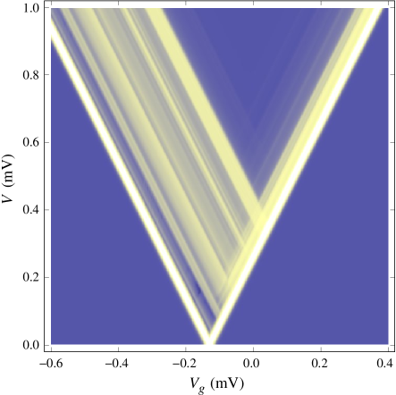
Figure 8: (Color online) Differential conductance per molecule averaged over all magnetic-field directions, $\overline{g}$, as a function of gate voltage $V_{g}$ and bias voltage $V$. Bright (dark) colors denote $\overline{g}>0$ ($\overline{g}<0$). The parameters are identical to Fig. 1, except that the magnetic-field direction is not held fixed but is averaged over, and the same color scheme is used.

For orientation, we first show $\overline{g}(V_{g},V)$ for $S=2$ in Fig. 8. The plot should be compared to Fig. 1 for the same parameters except for fixed $\theta=45^{\circ}$ in Fig. 1. Figure 8 shows that a lot of the fine structure survives the angular averaging. Plots of this type could not be obtained experimentally, due to the lack of a gate electrode for a monolayer. What can be measured is the differential conductance $\overline{g}$ as a function of bias voltage for given onsite potential $\epsilon_{0}$. Large signals are expected if the particular molecule allows to reach the CB threshold with accessible bias voltages $V$.

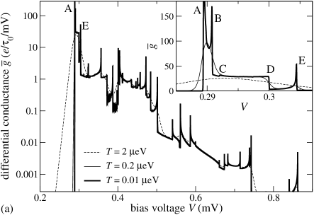
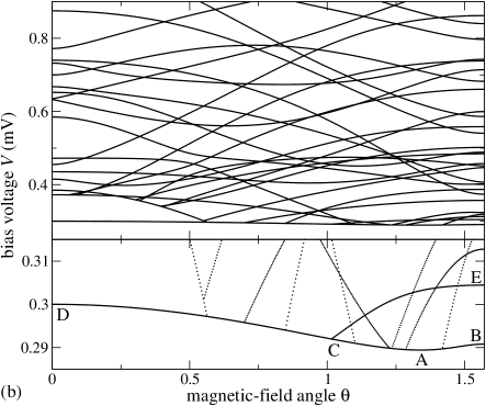
Figure 9: (a) Differential conductance per molecule averaged over all magnetic-field directions, $\overline{g}$, as a function of bias voltage $V$ at three temperatures. $\overline{g}$ is plotted on a logarithmic scale. The parameters are as in Fig. 6(b). The inset shows $\overline{g}$ in the vicinity of the CB threshold on a linear scale. Several van Hove singularities are marked. (b) Upper part: bias voltage of $g$ peaks as a function of magnetic-field angle $\theta$, for the same parameters. Lower part: close-up of the vicinity of the CB threshold. The points corresponding to the van Hove singularities in (a) are marked by the same letters.

Figure 9(a) shows $\overline{g}(V)$ for a monolayer of spin $S=2$ molecules in a magnetic field of magnitude $|\mathbf{H}|=0.1\,\mathrm{meV}$. This plot corresponds to Fig. 6(b) averaged over $\theta$ with the weight factor $\sin\theta$. We again see that the averaged differential conductance retains a lot of structure, in particular at very low temperatures. In the following, we analyze this structure in terms of van Hove singularities.

To help with this analysis, Fig. 9(b) shows the bias voltages of $g$ peaks (current steps) as a function of magnetic-field angle $\theta$. These are the “bands” that lead to van Hove singularities. This is simply a map of $g$ peaks occuring in Fig. 6(b). The first, strong peak in Fig. 9(a) corresponds to the CB threshold. Figures 6(b) and 9(b) show that the CB threshold is angle-dependent. Singularity A stems from the minimum of the transition energy and B from the maximum at $\theta=\pi/2$. These are both of the typical one-dimensional form $1/\sqrt{|V-V_{c}|}$. The maximum at $\theta=0$ leads to singularity D, which is only a step, due to the weight factor $\sin\theta$. As noted above, the presence of a step shows that the transition is allowed for $\theta=0$. The $1/\sqrt{|V-V_{c}|}$ singularity E stems from the maximum of a transition not at the CB threshold.

In addition, there is weaker step C, which cannot be attributed to an extremum at $\theta=0$. Figure 9(b) shows that a transition can suddenly vanish when it intersects another one. This is a typical property of inelastic sequential tunneling through molecules, which is due to the initial state of one of the transitions being populated (at $T=0$) only on one side of the crossing. One can show that the sum of weights (current step heights) of the transitions is analytic through the crossing, as a function of $H_{x}$, $H_{z}$, $\theta$, or $V_{g}$.footnote.continuity This means that a three-way crossing can be viewed as the superposition of a band for which the energy and the weight are analytic functions of $\theta$ and another band for which the weight is analytic but the energy shows a kink (change of slope). This kink leads to a type of van Hove singularity not present in band structures for weakly interacting electrons in solids. It shows up as a kink in the current and thus as a step in $\overline{g}$. Singularity C in Fig. 9(a) is of this type, coming from the three-way crossing marked in Fig. 9(b). If both transitions have nonzero weight on both sides, part of the weight is also typically transferred from one band to the other, leading to the same type of singularity.

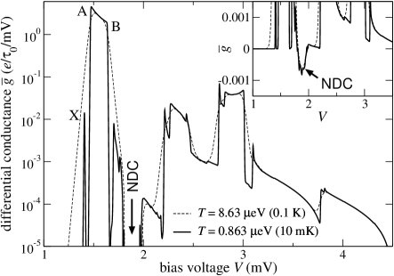
Figure 10: Differential conductance per molecule averaged over all magnetic-field directions, $\overline{g}$, as a function of bias voltage $V$ for a monolayer of $\mathrm{Mn}_{12}$ molecules with randomly oriented easy axes at two temperatures. $\overline{g}$ is plotted on a logarithmic scale. The inset shows $\overline{g}$ on a linear scale to exhibit the NDC region. Several van Hove singularities are marked, see text.

Finally, we turn to a monolayer of $\mathrm{Mn}_{12}$ molecules ($S=10$) with random easy axes. We consider the case corresponding to averaging $g$ in Fig. 7(a) over angles. The result is the differential conductance plotted in Fig. 10. The most prominent features are the step-like singularities A and B. B stems from the maximum of the transition energy of the strong low-bias peak in Fig. 7(a) at about $V=1.64\,\mathrm{mV}$. It is a step since the maximum occurs at $\theta=0$. However, singularity A is also a step, although it clearly results from the minimum of that transition energy at $\theta=\pi/2$ so that we expect a pole, $1/\sqrt{|V-V_{c}|}$. This can be understood by extending Fig. 7(a) to angles $\theta>\pi/2$ using reflection symmetry. The minimum is in fact a crossing between the transitions from $\langle S^{z}_{\mathrm{tot}}\rangle=\pm 10$ to $\pm 21/2$, i.e., the transitions out of the respective ground state and blocking state. Therefore singularity A is not of the form of a band extremum but of a band crossing, i.e., a step. The anomalous exponent of singularity A is thus closely related to the spin blockade discussed earlier.

The sharp peak X in Fig. 10 is an artifact coming from molecules with $\theta=0$, for which the CB threshold formally occurs at $V_{\mathrm{CB}}=1.41\,\mathrm{mV}$. Finally, the extended region of NDC in Fig. 7(a) leads to NDC even in the angle-averaged differential conductance, as seen in the inset of Fig. 10.

IV Summary and conclusions

In summary, we have studied inelastic electron tunneling through molecules with a local magnetic moment and large uniaxial anisotropy in a strong magnetic field. Since the orientation of the molecules is often not well controlled in tunneling experiments, we consider arbitrary angles between easy axis and field. Then the anisotropy and Zeeman terms in the Hamiltonian do not commute so that no component of the molecular spin is conserved. This lifts all spin selection rules for electron tunneling, leading to large numbers of allowed molecular transitions and consequently to many peaks in the differential conductance $g=dI/dV$. The resulting complex fine structure of Coulomb-diamond plots is already apparent for the relatively simple case of a local spin $S=2$.

As a concrete example, $\mathrm{Mn}_{12}$ molecules are studied. The large spin $S=10$ leads to even more complex fine structure. However, one can still attribute differential-conductance peaks to individual molecular transitions. It should be possible to analyze experimental results in terms of specific molecular transitions if one has a model for guidance. Even without detailed attribution of observed peaks, measurement of $g$ in magnetic fields of various directions should allow to determine the orientation of the molecule relative to the leads, which is not directly accessable in break-junction or electromigration experiments.

We have considered three cases: Single molecules, molecular monolayers with aligned easy axes, and molecular monolayers with random easy axes. For monolayers one does not have the advantage of a gate electrode. However, one can extract similarly detailed information by varying the magnetic field. For randomly oriented molecules we have found that the averaging of transition energies over orientations leads to van Hove singularities in $g$. Besides the normal singularities from extrema of “bands,” a novel type arises from crossings of transition energies. Analysis of the singularities can give rather detailed information on allowed vs. forbidden transitions in the limit of the easy axis aligned with the magnetic field and on the presence of blocking states (spin blockade).

Detailed calculations of $g$ for $\mathrm{Mn}_{12}$ with its many molecular states and in particular for monolayers with random orientation are made feasible by an approximation scheme for solving the rate equations. As further results, we predict large and highly anisotropic magnetoresistance at low temperatures, if the bias voltage is tuned close to the CB threshold, and negative differential conductance, which survives even for randomly oriented monolayers of $\mathrm{Mn}_{12}$.

Appendix A Approximate solution of the rate equations

At $T=0$ we employ the following algorithm: For bias $V=0$, the molecular ground states have probability $1/d$, where $d$ is the ground-state degeneracy, and the current vanishes. For increasing $V$, the current remains zero in the sequential-tunneling approximation until $eV/2$ reaches the energy $\Delta\epsilon$ of the first allowed transition starting from a ground state. Above this value, all states obtain nonzero probabilities that can be reached from a ground state directly or indirectly by allowed and energetically possible transitions. The network of these states is constructed by testing all possible transitions. Then the matrix $A$ above the threshold $eV/2=\Delta\epsilon$ is obtained from Eq. (3), taking into account that the Fermi factors are $f=0$ or $1$. $A$ is then diagonalized. This is faster and more robust than in the general case because (a) the dimension of $A$ is smaller since it only contains active states and (b) $A$ does not contain exponentially small components—all components are either exactly zero or given by matrix elements. The resulting current is calculated from Eq. (4). The value of $\Delta\epsilon$ and the change (step height) in the current are recorded. Then we go over to the next bias for which $eV/2$ equals a transition energy, extend the network of states by all states that can now be reached, obtain $A$, diagonalize it, and calculate the new current. These steps are repeated.

Note that we only diagonalize $H_{\mathrm{mol}}$ once to obtain the transition energies and matrix elements. Furthermore, we only diagonalize $A$ once for each transition energy, since the current at $T=0$ is constant between steps. The result is a list of bias voltages $V_{i}$ and associated heights $g_{i}$ of current steps. The $g_{i}$ are also the weights of delta-function peaks in $g=dI/dV$.

To obtain approximate results at finite, but low, temperatures, we broaden the current steps so that their width is of the order of $k_{B}T$. We write the current as

$$I\approx e\sum_{i}g_{i}\,\left[f\!\left(\frac{eV_{i}-eV}{2k_{B}T}\right)-f\!\left(\frac{eV_{i}+eV}{2k_{B}T}\right)\right],$$ (7)

where $i$ enumerates the current steps. This particular broadening function is chosen since Eq. (7) is exact (assuming sequential tunneling) for the simplest possible model, i.e., a single orbital for a spin-less fermion. The form of the broadened delta functions in $g$ follows trivially. The approximation is good if the separation in $eV/2$ between current steps is large compared to $k_{B}T$.

References

- (1) J. Park, A. N. Pasupathy, J. I. Goldsmith, C. Chang, Y. Yaish, J. R. Petta, M. Rinkoski, J. P. Sethna, H. D. Abruña, P. L. McEuen, and D. C. Ralph, Nature (London) 417, 722 (2002).
- (2) W. Liang, M. P. Shores, M. Bockrath, J. R. Long, and H. Park, Nature (London) 417, 725 (2002).
- (3) J. Paaske and K. Flensberg, Phys. Rev. Lett. 94, 176801 (2005).
- (4) F. Elste and C. Timm, Phys. Rev. B 71, 155403 (2005).
- (5) H. B. Heersche, Z. de Groot, J. A. Folk, H. S. J. van der Zant, C. Romeike, M. R. Wegewijs, L. Zobbi, D. Barreca, E. Tondello, and A. Cornia, Phys. Rev. Lett. 96, 206801 (2006).
- (6) C. Romeike, M. R. Wegewijs, W. Hofstetter, and H. Schoeller, Phys. Rev. Lett. 96, 196601 (2006); Phys. Rev. Lett. 97, 206601 (2006).
- (7) C. Romeike, M. R. Wegewijs, and H. Schoeller, Phys. Rev. Lett. 96, 196805 (2006).
- (8) M.-H. Jo, J. E. Grose, K. Baheti, M. M. Deshmukh, J. J. Sokol, E. M. Rumberger, D. N. Hendrickson, J. R. Long, H. Park, and D. C. Ralph, Nano Lett. 6, 2014 (2006).
- (9) C. Timm and F. Elste, Phys. Rev. B 73, 235304 (2006).
- (10) F. Elste and C. Timm, Phys. Rev. B 73, 235305 (2006).
- (11) M. N. Leuenberger and E. R. Mucciolo, Phys. Rev. Lett. 97, 126601 (2006).
- (12) A. Donarini, M. Grifoni, and K. Richter, Phys. Rev. Lett. 97, 166801 (2006).
- (13) M. Misiorny and J. Barnas, eprint cond-mat/0610556 (unpublished).
- (14) G. Gonzalez and M. N. Leuenberger, eprint cond-mat/0610653 (unpublished).
- (15) F. Elste and C. Timm, Phys. Rev. B (submitted), eprint cond-mat/0611108.
- (16) C. Joachim, J. K. Gimzewski, and A. Aviram, Nature (London) 408, 541 (2000).
- (17) W. Harneit, Phys. Rev. A 65, 032322 (2002).
- (18) Y. Xue and M. A. Ratner, in Nanotechnology: Science and Computation, edited by J. Chen, N. Jonoska, and G. Rozenberg (Springer-Verlag, Berlin, 2006).
- (19) K. Blum, Density Matrix Theory and Applications (Plenum, New York, 1981).
- (20) H. Schoeller and G. Schön, Phys. Rev. B 50, 18436 (1994).
- (21) J. König, H. Schoeller, and G. Schön, Europhys. Lett. 31, 31 (1995).
- (22) M. Turek and K. A. Matveev, Phys. Rev. B 65, 115332 (2002).
- (23) H. Bruus and K. Flensberg, Many-body Quantum Theory in Condensed Matter Physics (Oxford University Press, Oxford, 2004).
- (24) A. Mitra, I. Aleiner, and A. J. Millis, Phys. Rev. B 69, 245302 (2004).
- (25) J. Koch, F. von Oppen, Y. Oreg, and E. Sela, Phys. Rev. B 70, 195107 (2004).
- (26) J. Koch and F. von Oppen, Phys. Rev. Lett. 94, 206804 (2005).
- (27) K. Park and M. R. Pederson, Phys. Rev. B 70, 054414 (2004).
- (28) J. R. Friedman, M. P. Sarachik, J. Tejada, and R. Ziolo, Phys. Rev. Lett. 76, 3830 (1996).
- (29) K. M. Mertes, Y. Suzuki, M. P. Sarachik, Y. Myasoedov, H. Shtrikman, E. Zeldov, E. M. Rumberger, D. N. Hendrickson, and G. Christou, Solid State Commun. 127, 131 (2003).
- (30) B. Fleury, L. Catala, V. Huc, C. David, W. Z. Zhong, P. Jegou, L. Baraton, S. Palacin, P.-A. Albouy, and T. Mallah, Chem. Commun. (Cambridge) 2005, 2020.
- (31) W. H. Zurek, Phys. Rev. D 26, 1862 (1982).
- (32) T. L. Hill, J. Theor. Biol. 10, 399 (1966).
- (33) J. Schnakenberg, Rev. Mod. Phys. 48, 571 (1976).
- (34) R. K. P. Zia and B. Schmittmann, J. Phys. A: Math. Gen. 39, L407 (2006).
- (35) The higher-energy multiplet of states with , which is split from the lower multiplet by an energy of order , also becomes occupied due to tiny matrix elements between states with large negative and states with large positive . However, the probabilities are negligible for the present discussion.
- (36) There is another multiplet of states at higher energies, split from the low-energy multiplet by a large energy of the order of . These states are not populated for the bias voltages considered here.
- (37) X. H. Qiu, G. V. Nazin, and W. Ho, Phys. Rev. Lett. 92, 206102 (2004).
- (38) A significant number of electrons have to tunnel through the molecule for it to get from the ground state to the state with , but after that it is essentially trapped and the stationary current is very small.
- (39) This follows because the current at is analytic, as long as no transition is crossed, since the Fermi functions are then constant and the matrix elements are analytic functions of magnetic field and gate voltage.