Line Shape Broadening in Surface Diffusion of Interacting Adsorbates
with Quasielastic He Atom Scattering

Abstract

The experimental line shape broadening observed in adsorbate diffusion on metal surfaces with increasing coverage is usually related to the nature of the adsorbate-adsorbate interaction. Here we show that this broadening can also be understood in terms of a fully stochastic model just considering two noise sources: (i) a Gaussian white noise accounting for the surface friction, and (ii) a shot noise replacing the physical adsorbate-adsorbate interaction potential. Furthermore, contrary to what could be expected, for relatively weak adsorbate-substrate interactions the opposite effect is predicted: line shapes get narrower with increasing coverage.

The diffusion of atoms, molecules, or small clusters on metal surfaces is an elementary dynamical process of paramount importance; it constitutes the ground step to understanding more complex phenomena in surface science. Processes such as heterogeneous catalysis, molecular-beam epitaxy, crystal growth, chemical vapor deposition, or associative desorption are all strongly affected by the kinetics of diffusion. Different experimental techniques have been used to study activated surface diffusion gomer ; eli ; jardine1 , quasielastic helium-atom scattering (QHAS) being one of the most valuable for such a purpose toennies1 ; toennies2 ; toennies3 . In QHAS experiments the observable is the so-called differential reflection coefficient. In analogy to neutron scattering by liquids vanHove , this magnitude gives the probability that the He-atom beam scattered from the diffusing collective reaches a solid angle $\Omega$ with an energy exchange $\hbar\omega$=$E_{f}-E_{i}$ and parallel (to the surface) momentum transfer $\Delta{\bf K}$=${\bf K}_{f}-{\bf K}_{i}$, and is proportional to the dynamic structure factor or scattering law, $S(\Delta{\bf K},\omega)$. $S(\Delta{\bf K},\omega)$ provides information about the dynamics and structure of the adsorbates, thus allowing to better understand the nature of adsorbate-substrate toennies2 and adsorbate-adsorbate toennies3 interactions. In general, $S(\Delta{\bf K},\omega)$ usually consists of the quasielastic ($Q$) peak and some weaker peaks attributed to the diffusion process and to phonon excitations and adsorbate low frequency vibrational modes [namely, the frustrated translational ($T$) modes], respectively.

Here we present a novel and insightful stochastic approach that allows to study and understand in a simple manner how the adsorbate coverage influences $S(\Delta{\bf K},\omega)$. This approach, grounded on the theory of spectral-line collisional broadening developed by Van Vleck and Weisskopf weiss and the elementary kinetic theory of gases mcquarrie in the Langevin framework, relies on three assumptions: (i) the adsorbate-substrate interaction is described by a (deterministic) adiabatic adsorption potential, (ii) the temperature dependent nonadiabatic coupling to the substrate electronic and vibrational excitations is accounted for by a Gaussian white noise, and (iii) adsorbate-adsorbate interactions are described by a shot noise gardiner ; hanggi2 , as proposed in Ref. pre-I, . We call this approach the interacting single adsorbate approximation. Gaussian white noise has been used to characterize the rich variety of different transport regimes in surface diffusion sancho . Within a similar context, the shot noise has been used to study thermal ratchets hanggi1 , mean first passage times iturbe , and jump distributions tommei .

To explain the line-shape broadening undergone by the $Q$ peak with increasing coverage ($\theta$), high demanding molecular dynamics calculations within the Langevin framework have been carried out toennies3 ; ying . Though the calculations could reproduce the trend with $\theta$, the dipole-dipole interaction potential considered was not able to correctly provide the experimental broadening observed. As we show here, this $\theta$-dependent behavior can also be reproduced by a simple collision model, with collisions being described by a shot noise. Note that, providing collective behaviors are not relevant (as happens, for instance, at low temperatures benedek ), adsorbates undergo a relatively large number of collisions for relatively long time scales reaching the statistical or stochastic limit. This proves that the nature of the adsorbate-adsorbate interaction could not be very relevant regarding the line shape broadening (as well as its trend). As seen here, the broadening is strikingly related to the surface corrugation (which strongly couples diffusion and low frequency vibrations) as well as to the friction associated to increasing $\theta$. This important result emerges when combining the numerical simulations using our model with a fully analytical treatment, which allows to understand and to interpret the process in terms of two limiting cases: running or diffusive and bound trajectories risken .

The starting point of our approach consists of expressing the dynamic structure factor as vanHove ; JLvega1

$$S(\Delta{\bf K},\omega)=\int e^{-i\omega t}\ \!I(\Delta{\bf K},t)dt,$$ (1)

where

$$I(\Delta{\bf K},t)=\langle e^{-i\Delta{\bf K}\cdot[{\bf R}(t)-{\bf R}(0)]}\rangle=\langle e^{-i\Delta K\!\int_{0}^{t}v_{\Delta{\bf K}}(t^{\prime})dt^{\prime}}\rangle$$ (2)

is the intermediate scattering function. In (2), the brackets denote an ensemble average and $v_{\Delta{\bf K}}$ is the adparticle velocity projected onto the $\Delta{\bf K}$ direction ($\Delta K$=$\|\Delta{\bf K}\|$). After a second order cumulant expansion in $\Delta K$ in the right-hand side (rhs) of the second equality of (2), one obtains

$$I(\Delta{\bf K},t)\approx e^{-\Delta K^{2}\!\int_{0}^{t}(t-t^{\prime})\mathcal{C}(t^{\prime})dt^{\prime}},$$ (3)

where $\mathcal{C}(t)$ = $\langle v_{\Delta{\bf K}}(0)v_{\Delta{\bf K}}(t)\rangle$ is the velocity autocorrelation function. This is the so-called Gaussian approximation mcquarrie , which is exact when velocity correlations of third or higher order are negligible. Despite its limitations, it provides much insight into the dynamical process by allowing an analytical treatment of the problem.

Determining the line shape of $S(\Delta{\bf K},\omega)$ through (1) thus requires us to simulate the adsorbate dynamics. This is done within a purely Langevin framework that includes the three elements mentioned above. Considering one dimension for simplicity, the motion of an adsorbate interacting with another adsorbates and a temperature-dependent substrate is ruled by the generalized Langevin equation hanggi2

$$\ddot{x}(t)=-\int_{0}^{t}\eta(t-t^{\prime})\ \!\dot{x}(t^{\prime})\ \!dt^{\prime}+F[x(t)]+\delta R(t),$$ (4)

where $x$ is the adsorbate coordinate, $\eta(t)$ is the memory function, $F$=$-\nabla V$ is the deterministic force per mass unit ($V$ is the periodic adsorbate-surface interaction potential, with period $a$), and $\delta R(t)$=$\delta R_{G}(t)$+$\delta R_{S}(t)$ is the noise source ($G$ and $R$ refer to Gaussian white noise and shot noise, respectively).

Gaussian white noise is defined by $\langle R_{G}(t)\rangle$=0 and $\langle R_{G}(t)R_{G}(t^{\prime})\rangle$=$2m\gamma k_{B}T\delta(t^{\prime}-t)$, where $m$ is the adsorbate mass, $T$ is the surface temperature, and $\gamma$ is the (constant) friction coefficient measuring the strength of the adsorbate-substrate coupling. On the other hand, the shot noise term in our model is $R_{S}(t)$=$\sum_{k=1}^{K}b_{k}(t-t_{k})$, where $b_{k}(t-t_{k})$=$c_{k}\lambda^{\prime}{\rm e}^{-\lambda^{\prime}(t-t_{k})}$ is the pulse or impact shape, with $t-t_{k}$$>$0 and $c_{k}$ giving the intensity of the collision impact. The pulse shape indicates that collisions are assumed to be sudden (strong but elastic) and after-collision effects relax exponentially at a constant rate $\lambda^{\prime}$. The probability for $K$ collisions to happen after a time $\mathcal{T}$ follows a Poisson distribution gardiner , $P_{K}(\mathcal{T})$=$(K!)^{-1}(\lambda\mathcal{T})^{K}e^{-\lambda\mathcal{T}}$, where $\lambda$ means the average number of collisions per time unit. Since collisions take place randomly at different orientations and energies, we reasonably assume $g(c_{k})$=$\alpha^{-1}e^{-c_{k}/\alpha}$, with $c_{k}$$\geq$0 and $\alpha$=$\sqrt{m/k_{B}T}$ pre-I .

The rate $\lambda^{\prime}$ defines a decay time scale for each collision event, $\tau_{c}$=$1/\lambda^{\prime}$. If $\tau_{c}$ is relatively small (collision effects relax relatively fast), the memory function associated to the shot noise in (4) is also local in time. Then, $\eta(t-t^{\prime})$$\simeq$$\eta\ \!\delta(t-t^{\prime})$ and, resorting to the Markovian approximation gardiner , Eq. (4) reduces to

$$\ddot{x}(t)=-\eta\dot{x}(t)+F[x(t)]+\delta R(t),$$ (5)

with a total constant friction $\eta$=$\gamma$+$\lambda$ and where $\langle\delta R(t)\delta R(t^{\prime})\rangle$=$2m\eta k_{B}T\delta(t^{\prime}-t)$. To estimate the value of $\lambda$, the elementary kinetic theory of transport in gases mcquarrie can be considered, where diffusion is proportional to the mean free path $\bar{l}$, and the latter is proportionally inverse to both the density of gas particles and the effective collision area when a hard-sphere model is assumed. By means of simple arguments pre-I , it is possible to find an also simple relationship between $\lambda$ and $\theta$, given by $\lambda$=$(6\rho\theta/a^{2})\sqrt{k_{B}T/m}$. Accordingly, increasing $\theta$ (and/or $T$) means an also increase of the collision frequency.

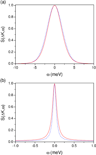
Figure 1: (Color online.) $Q$ peak for Na on Cu(001) at $\Delta K$=1.23 Å^-1, $T$=200 K, and $\theta_{1}$=0.028 (blue dashed line) and $\theta_{2}$=0.18 (red solid line). (a) Flat surface potential ($V$=0) and (b) non separable corrugated potential toennies2 .

In Fig. 1 we have plotted 2D calculations for $S(\Delta{\bf K},\omega)$ with two different types of corrugation: (a) low corrugation, assuming $V$=0, and (b) a non separable corrugated potential toennies2 . We have considered Na on Cu(001) at $\Delta K$=1.23 Å^-1, surface temperature of 200 K and two coverages, $\theta_{1}$=0.028 and $\theta_{2}$=0.18, as in the experiment toennies3 . After calculating 2D trajectories from Eq. (5), $I(\Delta{\bf K},t)$ is obtained using the rhs of the first equality in Eq. (2) and fitted to a certain analytical function (see below). Finally, the Fourier transform of that function gives $S(\Delta{\bf K},\omega)$. As is clearly seen in Fig. 1(a), the $Q$ peak gets narrower as $\theta$ increases for low corrugation. On the contrary, the presence of a potential leads to the broadening observed in Fig. 1(b). For instance, the full widths at half maximum (FWHM) for three coverages at $\Delta K$=1.26 Å^-1 are: $\Gamma$=120, 190, and 240 $\mu$eV for $\theta$=0.028, 0.106, and 0.18, which are in good agreement with the experimental ones, $\Gamma$=110, 150, and 270 $\mu$eV, respectively; these widths differ from those found in Ref. toennies3, ($\Gamma$=110, 130, and 160 $\mu$eV, respectively) by using a dipole-dipole interaction in Langevin molecular dynamics simulations.

To understand our results we can resort to two (analytical) limit cases: pure diffusion and anharmonic oscillations. After assuming $V$=0 in Eq. (5), one easily obtains $\mathcal{C}(t)$=$\langle v_{0}^{2}\rangle e^{-\eta t}$ (where $\langle v_{0}^{2}\rangle$=$k_{B}T/m$), which leads to

$$I(\Delta{\bf K},t)=\exp\left[-\chi^{2}\left(e^{-\eta t}+\eta t-1\right)\right]$$ (6)

after using Eq. (3) with $\chi^{2}$=$\langle v_{0}^{2}\rangle\Delta K^{2}/\eta^{2}$. On the other hand, for a damped harmonic oscillator JLvega1 ; risken we have $\mathcal{C}(t)$=$\langle v_{0}^{2}\rangle e^{-\eta t/2}\cos(\bar{\omega}t+\delta)/\cos\delta$, with $\bar{\omega}$=$\sqrt{\omega_{0}^{2}-(\eta/2)^{2}}$, $\delta$=$(\tan)^{-1}(\eta/2\bar{\omega})$, and $\omega_{0}$ being the harmonic frequency. Again, using Eq. (3), we obtain

$$I(\Delta{\bf K},t)=\exp\left\{-\frac{\chi^{2}\eta^{2}}{\bar{\omega}\omega_{0}}\left[\cos\delta-e^{-\eta t/2}\cos(\bar{\omega}t-\delta)\right]\right\}.$$ (7)

Unlike (6), Eq. (7) displays an oscillatory but exponentially damped behavior which does not decay to zero. Nevertheless, it approaches (6) in the limit $\omega_{0}\to 0$. Here we are not interested in the damped harmonic oscillator, but in an anharmonic one, which arises when the parameters in (7) are left free.

If deviations from the Gaussian approximation are not very important, $I(\Delta{\bf K},t)$ will display features typical of the behaviors described by both (6) and (7). Indeed, even if the Gaussian approximation does not hold, one can still make use of a working formula in order to extract relevant information about the process from the numerical results. Trajectories display both temporary trapping in potential wells and periods of time where the flight is unbound. Therefore, assuming a model of running ($R$) and bound ($B$) trajectories, one can consider $\mathcal{C}(t)$=$\alpha\mathcal{C}_{R}(t)+(1-\alpha)\mathcal{C}_{B}(t)$, where $\mathcal{C}_{R}$ and $\mathcal{C}_{B}$ correspond to the velocity autocorrelation functions for a flat surface and a damped anharmonic oscillator, respectively. $I(\Delta{\bf K},t)$ can be then written as

$$I(\Delta{\bf K},t)\approx[I_{R}(\Delta{\bf K},t)]^{\alpha}[I_{B}(\Delta{\bf K},t)]^{1-\alpha},$$ (8)

where $I_{R}$ and $I_{B}$ are given by Eqs. (6) and (7), respectively. This expression, with free parameters, is used as our working formula and allows for a distinction between the contributions arising from the unbound or diffusive motion and the bound or vibrational one.

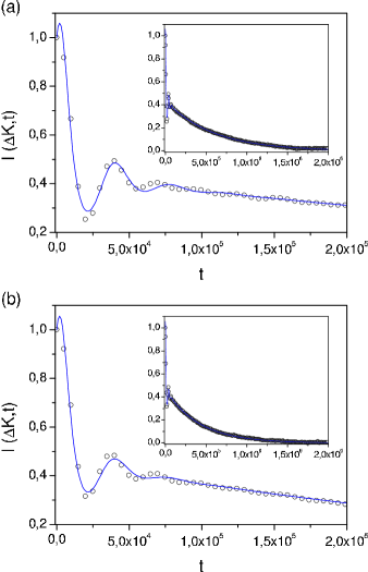
Figure 2: (Color online.) $I(\Delta{\bf K},t)$ for Na on Cu(001) at $\Delta K=1.23$ Å^-1, $T$=200 K, and (a) $\theta_{1}$=0.028 and (b) $\theta_{2}$=0.18. Open circles indicate the numerical values obtained from the simulation and solid lines are the numerical fitting using Eq. (8).

As seen in Fig. 2, Eq. (8) fits fairly well the Langevin numerical results obtained for the corrugated surface potential [see Fig. 1(b)] and both coverages. The fitting parameters compared with the nominal values are given in Table 1; though fitted and nominal values are different, their order of magnitude and trend are correct, regarding such differences to deviations from the Gaussian approximation. More importantly is, however, the resulting value for $\alpha$: $\alpha_{1}$=0.0294 for $\theta_{1}$, and $\alpha_{2}$=0.0410 for $\theta_{2}$. From these values, it is clear that the contribution to $I(\Delta{\bf K},t)$ primarily comes from bound motions. Note from (6) that running trajectories lead to a relative much faster decay of $I(\Delta{\bf K},t)$ than the bound motion [see Eq. (7)], which delays such a decay. This is so because the bound motion keeps correlations for times longer than the diffusive one, since the latter provokes a fast dephasing of the (correlation) oscillating terms that appear in the rhs of the first equality in Eq. (2). In this way, this explains, first, that $S(\Delta{\bf K},\omega)$ is about two orders of magnitude broader in the flat case than in the corrugated one (see Fig. 1). And, second, since $\alpha_{2}$$>$$\alpha_{1}$ there is a slightly larger fraction of running trajectories for $\theta_{2}$, which leads to an also slightly faster decay of $I(\Delta{\bf K},t)$, and therefore to observe broadening in $S(\Delta{\bf K},\omega)$ with increasing $\theta$. It is also worth stressing that, with increasing coverage, diffusion decreases (according to Einstein’s relation, it goes like $\eta^{-1}$) and the running trajectories display short flights in small surface regions.

coverage		$\omega$ (a.u.)		$\eta$ (a.u.)		$\delta$		$\chi$
$\theta_{1}^{\rm nom}$		2.20$\times$10-4		2.54$\times$10-5		0.058		3.15
$\theta_{1}^{\rm fit}$		1.39$\times$10-4		3.52$\times$10-5		0.184		4.64
$\theta_{2}^{\rm nom}$		2.19$\times$10-4		4.69$\times$10-5		0.107		1.71
$\theta_{2}^{\rm fit}$		1.37$\times$10-4		4.28$\times$10-5		0.276		2.82

Table 1: Nominal and fitted values involved in the calculation of $I(\Delta{\bf K},t)$ for $\theta_{1}$=0.028 and $\theta_{2}$=0.18.

To conclude, the simple stochastic model together with the theoretical analysis presented in this work shows that the experimental broadening observed in the $Q$ peak with increasing $\theta$ (from low to intermediate regimes) is related to the bound motion undergone by the adsorbates inside the potential wells, and not only to purely diffusive motion or to the particular form assumed for adsorbate-adsorbate interactions. Moreover, regardless the adsorbate-substrate interaction potential, in our model the line shape of $S(\Delta{\bf K},\omega)$ is also related to $\eta$, which gathers the thermal effects caused by the surface ($\gamma$) and the collisions among adsorbates ($\lambda$). Since $\gamma$ is assumed to be constant, the broadening is thus directly related to an increasing friction $\lambda$ as $\theta$ increases. The idea of replacing the dipole-dipole interaction by a shot noise is crucial because, for long time processes with a high number of collisions, the statistical limit seems to wipe out any trace of the true interaction potential. As happens with the models proposed in the literature toennies2 ; toennies3 ; benedek , ours gives a smaller diffusion than expected with increasing $\theta$, which could be related to the fact that $\theta$ might also influence the type of adsorbate-substrate interaction, and therefore modify parameters such as the activation barrier or the surface friction in our model. Thus, in Ref. benedek, , the Lau-Kohn long range interaction via intrinsic surface states is proposed to use a $\theta$-dependent surface electronic density modifying the corrugated potential and to explain the remarkable increasing of the $T$ mode frequency with coverage at 50 K which a dipole-dipole or substrate mediated coupling cannot explain it. This increasing is also observed at 200 K and parallel momentum transfer of $-2$ Å^-1 to be 11$\%$, which is similar to our value (around 7$\%$) when going from $\theta$=0.028 to 0.106 at 2.10 Å^-1. Although further investigation at microscopic level and calculations from first principles are needed, our simple stochastic model at low coverages and surface temperatures is also able to provide a complementary view of diffusion and low-frequency vibrational motions, described by the peaks around or near zero energy transfers in the scattering law.

This work has been supported in part by DGCYT (Spain) under project FIS2004-02461. R.M.-C. thanks the University of Bochum for support from the Deutsche Forschungsgemeinschaft, SFB 558, for a predoctoral contract. J.L.V. and A.S. Sanz would like to thank the Ministerio de Educación y Ciencia (Spain) for a predoctoral grant and a “Juan de la Cierva” Contract, respectively.

References

- eprint
- (1) R. Gomer, Rep. Prog. Phys. 53, 917 (1990).
- (2) S. Miret-Artés and E. Pollak, J. Phys.: Condens. Matter 17, S4133 (2005).
- (3) A.P. Jardine et al., Science 304, 1790 (2004); P. Fouquet et al., Rev. Sci. Inst. 76, 053109 (2005); G. Alexandrowicz et al., Phys. Rev. Lett. 97, 156103 (2006).
- (4) A. Graham, F. Hofmann, and J.P. Toennies, J. Chem. Phys. 104, 5311 (1996).
- (5) A.P. Graham et al., Phys. Rev. B 56, 10567 (1997).
- (6) J. Ellis et al., Phys. Rev. B 63, 195408 (2001).
- (7) L. van Hove, Phys. Rev. 95, 249 (1954).
- (8) J.H. van Vleck and V.F. Weisskopf, Rev. Mod. Phys. 17, 227 (1945).
- (9) D.A. McQuarrie, Statistical Mechanics (Harper and Row, New York, 1976).
- (10) C.W. Gardiner, Handbook of Stochastic Methods (Springer-Verlag, Berlin, 1983).
- (11) P. Hänggi and P. Jung, Adv. Chem. Phys. 89, 239 (1995).
- (12) R. Martínez-Casado et al., Phys. Rev. E 75, 05xxxx (2007).
- (13) J.M. Sancho et al., Phys. Rev. Lett. 92, 250601 (2004).
- (14) T. Czernik et al., Phys. Rev. E 55, 4057 (1997); J. Luczka et al., Phys. Rev. E 56, 3968 (1997).
- (15) F. Laio et al., Phys. Rev. E 63, 036105 (2001).
- (16) R. Ferrando et al., New J. Phys. 7, 19 (2005).
- (17) A. Cucchetti and S.C. Ying, Phys. Rev. B 60, 11110 (1999).
- (18) A.P. Graham, J.P. Toennies, and G. Benedek, Surf. Sci. 556, L143 (2004).
- (19) H. Risken, The Fokker-Planck Equation (Springer-Verlag, Berlin, 1984).
- (20) J.L. Vega, R. Guantes, and S. Miret-Artés, J. Phys.: Condens. Matter 14, 6193 (2002); ibid. 16, S2879 (2004).