Weak localization in a system with a barrier: Dephasing and weak Coulomb blockade

Abstract

We non-perturbatively analyze the effect of electron-electron interactions on weak localization (WL) in relatively short metallic conductors with a tunnel barrier. We demonstrate that the main effect of interactions is electron dephasing which persists down to $T=0$ and yields suppression of WL correction to conductance below its non-interacting value. Our results may account for recent observations of low temperature saturation of the electron decoherence time in quantum dots.

Electrons propagating in a disordered conductor get scattered and interfere. This quantum interference is possible only as long as the electron wave functions remain coherent. In any realistic situation, however, interactions between electrons and with other degrees of freedom may limit phase coherence and, hence, reduce electrons ability to interfere. The interplay between scattering, quantum coherence and interactions yields a rich variety of non-trivial effects and significantly impacts electron transport in disordered conductors.

The so-called weak localization (WL) correction to the conductance of a disordered system $G_{WL}$ is most sensitive to electron coherence and is known to arise from interference of pairs of time-reversed electron paths [1]. In a system of two scatterers separated by a cavity (quantum dot) and in the absence of interactions this correction can be directly evaluated [2]. The effect of electron-electron interactions can be described in terms of fluctuating voltages. Provided the voltage drops only across the barriers and not inside the cavity electron-electron interactions yield energy dependent logarithmic renormalization of the dot channel transmissions [3, 4] but do not cause any dephasing [5, 6]. The latter result can easily be understood if one observes that the voltage-dependent random phase acquired by the electron wave function $\Psi$ along any path turns out to be the same as that for its time-reversed counterpart. Hence, in the product $\Psi\Psi^{*}$ these random phases cancel each other exactly and quantum coherence of electrons remains preserved.

It is important, however, that this cancellation occurs only in the case of two scatterers, whereas in a system of three or more scatterers the situation is entirely different. Consider, e.g., a system of two quantum dots depicted in Fig. 1 and again assume that fluctuating voltages are concentrated at the barriers. The phase factor accumulated along the path (see Fig. 1) which crosses the central barrier twice (at times $t_{i}$ and $t>t_{i}$) and returns to the initial point (at a time $t_{f}$) is $e^{i[\varphi^{+}(t_{i})-\varphi^{+}(t)]}$, where $\dot{\varphi}^{+}/e=V(t)$ is the fluctuating voltage across the central barrier. Similarly, the phase factor picked up along the time-reversed path reads $e^{i[\varphi^{+}(t_{f}+t_{i}-t)-\varphi^{+}(t_{f})]}$. Hence, the overall phase factor acquired by the product $\Psi\Psi^{*}$ for a pair of time-reversed paths is $\exp(i\Phi_{\rm tot})$, where $\Phi_{\rm tot}(t_{i},t_{f},t)=\varphi^{+}(t_{i})-\varphi^{+}(t)-\varphi^{+}(t_{f}+t_{i}-t)+\varphi^{+}(t_{f})$. Averaging over phase fluctuations, which for simplicity are assumed Gaussian, we obtain

$$\left\langle e^{i\Phi_{tot}(t_{i},t_{f},t)}\right\rangle=\,e^{-\frac{1}{2}\left\langle\Phi_{tot}^{2}(t_{i},t_{f},t)\right\rangle}$$

$$=\,e^{-2F(t-t_{i})-2F(t_{f}-t)+F(t_{f}-t_{i})+F(t_{f}+t_{i}-2t)},$$ (1)

where we defined the phase correlation function

$$F(t)=\langle(\varphi^{+}(t)-\varphi^{+}(0))^{2}\rangle/2.$$ (2)

Should this function grow with time the electron phase coherence decays and $G_{WL}$ gets suppressed below its non-interacting value.

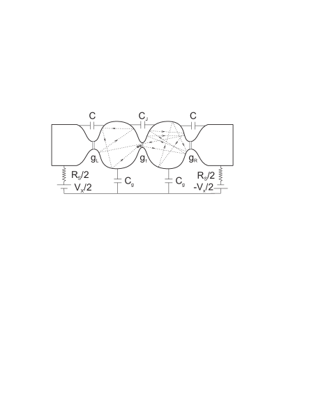
Figure 1: Two quantum dots separated by a tunnel barrier and connected to the battery $V_{x}$ via an Ohmic shunt resistor $R_{S}$.

The above arguments are not specific to the system of three barriers and after proper generalization can be applied to virtually any disordered conductor. At the same time, these arguments are not yet sufficient to quantitatively describe the decoherence effect of electron-electron interactions for two important reasons: (i) fluctuating voltages are treated as external (classical) fields rather than quantum fields produced internally by fluctuating electrons and (ii) Fermi statistics is not yet accounted for. Below we will cure both these problems and non-perturbatively evaluate WL correction $G_{WL}$ for a metallic system with a tunnel barrier and (at least) two more scatterers in the presence of electron-electron interactions which turn out to reduce phase coherence of electrons at any temperature down to $T=0$.

We will consider a system with a tunnel barrier with dimensionless conductance $g_{t}$, which separates two sufficiently short disordered metallic conductors with Thouless energies $E_{\rm Th}$ and dimensionless conductances $g_{L,R}\gg 1,g_{t}$. This system is described by the Hamiltonian

$$\hat{\bm{H}}=\hat{\bm{H}}_{L}+\hat{\bm{H}}_{R}+\hat{\bm{T}}+\hat{\bm{H}}_{em},$$ (3)

where $\hat{\bm{H}}_{L,R}=\sum_{\alpha=\uparrow,\downarrow}\int_{L,R}d^{3}{\bm{r}}\,\hat{\Psi}_{\alpha;L,R}^{\dagger}({\bm{r}})\hat{H}_{L,R}\hat{\Psi}_{\alpha;L,R}({\bm{r}})$ is the Hamiltonian of the left (right) lead, $\hat{H}_{L,R}=-\frac{\nabla^{2}}{2m_{L,R}}-\mu+U_{imp}({\bm{r}})$ is the single electron Hamiltonian in the left (right) lead, and $\hat{T}=\sum_{\alpha=\uparrow,\downarrow}\int_{J}d^{2}{\bm{r}}\left[t({\bm{r}})e^{-i\hat{\varphi}(t)}\hat{\Psi}_{\alpha;L}^{\dagger}({\bm{r}})\hat{\Psi}_{\alpha;R}({\bm{r}})+c.c.\right]$ is the tunnel Hamiltonian. Here $\hat{\varphi}$ is the phase operator, which is related to the voltage drop across the junction $\hat{\varphi}(t)=\int^{t}_{t_{0}}dt^{\prime}e\hat{V}(t^{\prime})$, and the ${\bm{r}}$-integration runs over the junction area. Finally, $\hat{\bm{H}}_{em}\propto\hat{V}^{2}$ is the quadratic Hamiltonian of electromagnetic fields, the precise form of which depends on the circuit configuration and will not be specified here.

Following the standard procedure we integrate out fermionic degrees of freedom and arrive at the effective action $iS=2\,{\rm Tr}\,\ln\left[\check{G}^{-1}\right]$, where $\check{G}$ is the Green-Keldysh function for our system. Expanding the action in powers of the tunnel Hamiltonian we obtain $S=S_{L,R}+S^{(1)}_{t}+S^{(2)}_{t}+...$, where the term $S_{L,R}$ describes the action of the left and right conductors, $S^{(1)}_{t}$ is Ambegaokar-Eckern-Schön action [7] and

$$iS^{(2)}_{t} = -\sum_{i,j,k,l=F,B}\int dt_{1}\dots dt_{4}\int_{J}d\bm{x}_{1}\dots d\bm{x}_{4}\,$$ (4)

$$\times\,\check{G}_{L,ij}(X_{1};X_{2})(-1)^{j}e^{-i\varphi_{j}(t_{2})}t(\bm{x}_{2})\times\,\check{G}_{R,jk}(X_{2};X_{3})(-1)^{k}e^{i\varphi_{k}(t_{3})}t(\bm{x}_{3})$$

$$\times\,\check{G}_{L,kl}(X_{3};X_{4})(-1)^{l}e^{-i\varphi_{l}(t_{4})}t(\bm{x}_{4})\times\,\check{G}_{R,li}(X_{4};X_{1})(-1)^{i}e^{i\varphi_{i}(t_{1})}t(\bm{x}_{1}).$$

Here $X=(t,\bm{x})$, $\varphi_{F(B)}$ is the phase variable on the forward (backward) branch of the Keldysh contour, $\check{G}_{r}$ are $2\times 2$ matrix Green-Keldysh functions in the left and right conductors ($r=L,R$) and we use the convention $(-1)^{F}=-1$, $(-1)^{B}=1$. We assume that $\check{G}_{L,R}$ have the equilibrium form $\check{G}_{r}=G_{r}^{R}\check{F}_{1}-\check{F}_{2}G_{r}^{A}$, where $G^{R,A}_{r}$ are retarded and advanced Green functions,

$$\check{F}_{1}(E)=\left(\begin{array}[]{cc}h(E)&-f(E)\\ h(E)&-f(E)\end{array}\right),$$

$$\check{F}_{2}(E)=\left(\begin{array}[]{cc}f(E)&f(E)\\ -h(E)&-h(E)\end{array}\right),$$

$f(E)$ is the Fermi function and $h(E)=1-f(E)$.

Our next step amounts to averaging the products of retarded and advanced propagators in the action (4) over disorder in each conductor separately. We have (see, e.g., [8])

$$\langle G^{R}_{L}(X_{1},X_{2})G^{A}_{L}(X_{3},X_{4})\rangle=\langle G^{R}_{L}(X_{1},X_{2})\rangle\langle G^{A}_{L}(X_{3},X_{4})\rangle$$

$$+\,2\pi N_{L}w(|\bm{r}_{1}-\bm{r}_{4}|)w(|\bm{r}_{2}-\bm{r}_{3}|)\times\,{\cal D}_{L}\left(t_{1}-t_{2};\frac{\bm{r}_{1}+\bm{r}_{4}}{2},\frac{\bm{r}_{2}+\bm{r}_{3}}{2}\right)$$

$$\times\delta(t_{1}-t_{2}+t_{3}-t_{4})+\,2\pi N_{L}w(|\bm{r}_{1}-\bm{r}_{3}|)w(|\bm{r}_{2}-\bm{r}_{4}|)$$

$$\times\,{\cal C}_{L}\left(t_{1}-t_{2};\frac{\bm{r}_{1}+\bm{r}_{3}}{2},\frac{\bm{r}_{2}+\bm{r}_{4}}{2}\right)\delta(t_{1}-t_{2}+t_{3}-t_{4}),$$ (5)

where $N_{L}$, ${\cal D}_{L}(t,\bm{r},\bm{r}^{\prime})$ and ${\cal C}_{L}(t,\bm{r},\bm{r}^{\prime})$ are respectively the density of states, the diffuson and the Cooperon in the left conductor, $w(r)=e^{-r/2l_{e}}\sin k_{F}r/k_{F}r$, $k_{F}$ and $l_{e}$ are respectively the Fermi wave vector and elastic mean free path. The same averaging procedure applies to the right conductor.

Finally we assume that the transmission amplitude $t(\bm{x})$ is random, quickly oscillating real function. Averaging over these oscillations yields $\overline{t(\bm{x})t(\bm{y})}=\delta(\bm{x}-\bm{y}){g_{t}(\bm{x})}/{8\pi^{2}N_{L}N_{R}}$, where $g_{t}(\bm{x})$ is the local conductance of the barrier. After all these steps Eq. (4) reduces to a sum of different terms. Here we will select only the terms responsible for weak localization which involve the product of two Cooperons ${\cal C}_{L}$ and ${\cal C}_{R}$. Collecting all such contributions we obtain

$$iS_{WL}=-i\int dt_{1}\dots dt_{4}\int d\tau_{1}d\tau_{2}\int_{J}d{\bm{x}}d{\bm{y}}$$

$$\times\,\frac{g_{t}({\bm{x}})g_{t}({\bm{y}})}{4\pi^{2}N_{L}N_{R}}\;{\cal C}_{L}(t_{1}-\tau_{1},{\bm{y}},{\bm{x}}){\cal C}_{R}(t_{2}-\tau_{2},{\bm{x}},{\bm{y}})\times\,e^{i\Phi(t_{1},...,t_{4})}\sin\frac{\varphi^{-}(t_{1})}{2}$$

$$\times\,\left[h(\tau_{1}-t_{2})e^{-i\frac{\varphi^{-}(t_{2})}{2}}+f(\tau_{1}-t_{2})e^{i\frac{\varphi^{-}(t_{2})}{2}}\right]$$

$$\times\,\left[h(\tau_{2}-t_{3})e^{i\frac{\varphi^{-}(t_{3})}{2}}f(t_{1}+t_{3}-t_{4}-\tau_{1})\right.$$

$$\left.-\,f(\tau_{2}-t_{3})e^{-i\frac{\varphi^{-}(t_{3})}{2}}h(t_{1}+t_{3}-t_{4}-\tau_{1})\right]$$

$$\times\,\left[e^{-i\frac{\varphi^{-}(t_{4})}{2}}f(-t_{1}+t_{2}+t_{4}-\tau_{2})+\,e^{i\frac{\varphi^{-}(t_{4})}{2}}h(-t_{1}+t_{2}+t_{4}-\tau_{2})\right]$$

$$+\,\big{\{}L\leftrightarrow R,\varphi^{\pm}\to-\varphi^{\pm}\big{\}}.$$ (6)

Here we defined “classical” $\varphi^{+}=(\varphi_{F}+\varphi_{B})/2$ and “quantum” $\varphi^{-}=\varphi_{F}-\varphi_{B}$ phases and introduced

$$\Phi(t_{1},...,t_{4})=\varphi^{+}(t_{1})-\varphi^{+}(t_{2})+\varphi^{+}(t_{3})-\varphi^{+}(t_{4})$$

and $f(t)=\int(dE/2\pi)\,f(E)e^{-iEt}\equiv\delta(t)-h(t)$. The action (6) fully accounts for the effects of electron-electron interactions on WL via the fluctuating phases $\varphi^{\pm}$.

In order to find the WL correction to the current across the central barrier $I_{WL}$ we make use of the following general formula

$$I_{WL}=ie\int D^{2}\varphi^{\pm}\,\frac{\delta iS_{WL}[\varphi^{\pm}]}{\delta\varphi^{-}}\,e^{iS_{L,R}+iS^{(1)}_{\rm t}}.$$ (7)

In the limit $g_{L,R}\gg 1,g_{t}$ this integral remains Gaussian in $\varphi^{\pm}$ at all relevant energies and can easily be performed. The effective expansion parameter in this case is $g_{t}^{2}/g_{L}g_{R}\ll 1$. Combining Eqs. (6) and (7) and introducing the average voltage at the barrier $V$ we find

$$I_{WL}=\frac{e}{8\pi^{3}N_{L}N_{R}}\,{\rm Re}\,\int_{J}d{\bm{x}}d{\bm{y}}\;g_{t}({\bm{x}})g_{t}({\bm{y}})\;\int dEd\omega_{1}d\omega_{2}d\omega_{3}\,$$

$$\times\,C_{R}(-\omega_{2},{\bm{x}},{\bm{y}})C_{L}(-\omega_{3},{\bm{y}},{\bm{x}})\times\,h(E-\omega_{2})f(E+eV+\omega_{3}-\omega_{1})$$

$$\times\,\big{[}f(E+eV-\omega_{1})h(E)P_{1}(\omega_{1},\omega_{2},\omega_{3})+\,f(E+eV-\omega_{1})f(E)P_{2}(\omega_{1},\omega_{2},\omega_{3})$$

$$+\,h(E+eV-\omega_{1})h(E)P_{2}(\omega_{1},\omega_{3},\omega_{2})$$

$$+\,h(E+eV-\omega_{1})f(E)P_{3}(\omega_{1},\omega_{2},\omega_{3})\big{]}-\,\big{\{}V\to-V\big{\}}.$$ (8)

Here $C_{L,R}$ and $P_{j}$ ($j=1,2,3$) are the Fourier transforms of respectively the Cooperons ${\cal C}_{L,R}(t)$ and the functions

$${\cal P}_{j}(t_{1},t_{2},t_{3})=\exp[-{\cal F}(t_{1},t_{2},t_{3})]{\cal Q}_{j}(t_{1},t_{2},t_{3}),$$ (9)

where

$${\cal F}=F(t_{1}+t_{3})+F(t_{3})+F(t_{1}+t_{2})+F(t_{2})$$

$$-F(t_{1}+t_{2}+t_{3})-F(t_{2}-t_{3})$$ (10)

and $F(t)=\langle(\hat{\varphi}(t)-\hat{\varphi}(0))^{2}\rangle/2$ coincides with the phase correlation function (2). The terms ${\cal Q}_{j}$ read

$${\cal Q}_{1}=e^{-i\left[K(t_{2})+K(t_{3})+K(|t_{2}-t_{3}|)\right]}$$

$$\times\,\big{\{}2e^{i\left[K(|t_{1}+t_{2}+t_{3}|)+K(t_{1}+t_{3})+K(t_{1}+t_{2})\right]}-\,e^{i\left[K(t_{1}+t_{2}+t_{3})+K(|t_{1}+t_{3}|)+K(|t_{1}+t_{2}|)\right]}\big{\}},$$

$${\cal Q}_{2}=e^{i\left[K(|t_{1}+t_{2}+t_{3}|)-K(t_{2})-K(|t_{3}|)\right]}e^{i\left[K(t_{1}+t_{3})-K(|t_{1}+t_{2}|)-K(t_{3}-t_{2})\right]},$$

$${\cal Q}_{3}=e^{i\left[K(t_{1}+t_{2}+t_{3})-K(|t_{2}|)-K(|t_{3}|)\right]}e^{-i\left[K(t_{1}+t_{3})+K(t_{1}+t_{2})-K(|t_{3}-t_{2}|)\right]},$$ (11)

where $K(t)=i\left\langle\big{[}\hat{\varphi}(0),\hat{\varphi}(t)\big{]}\right\rangle$ is the response function. Eqs. (8)-(11) represent the central result of our paper. They fully determine WL correction to the current in our system. The non-interacting result is reproduced by the first two lines of Eq. (8) before the square brackets, while the terms in the square brackets exactly account for the effect of interactions. The same result follows from the non-linear $\sigma$-model approach [9].

Our result demonstrates that the whole effect of electron-electron interactions is encoded in two different correlators of fluctuating phases $F(t)$ and $K(t)$. These correlation functions are well familiar from the so-called $P(E)$-theory [7, 10]. They read

$$F(t) = e^{2}\int\frac{d\omega}{2\pi}\,\omega\coth\frac{\omega}{2T}\,{\rm Re}\big{[}Z(\omega)\big{]}\frac{1-\cos\omega t}{\omega^{2}},$$ (12)

$$K(t) = e^{2}\int\frac{d\omega}{2\pi}\,{\rm Re}\big{[}Z(\omega)\big{]}\frac{\sin\omega t}{\omega},$$ (13)

where $Z(\omega)$ is an effective impedance “seen” by the central barrier. Both functions (12) and (13) are purely real and, hence, $|{\cal Q}_{j}|\leq 1$. At times $\tau_{RC}<|t|<1/E_{\rm Th}$ (an effective $RC$-time $\tau_{RC}$ will be defined later) we obtain $F(t)\simeq\frac{2}{g_{Z}}\left(\ln\left|\frac{\sinh\pi Tt}{\pi T\tau_{RC}}\right|+\gamma\right)$ and $K(t)\simeq\frac{\pi}{g_{Z}}\,{\rm sign}\,t$, where $g_{Z}=2\pi/e^{2}Z(0)=g_{0}+g_{t}$, $g_{0}^{-1}=g_{L}^{-1}+g_{R}^{-1}+e^{2}R_{S}/2\pi$ and $\gamma\simeq 0.577$ is the Euler constant. We observe that while $F(t)$ grows with time at any temperature including $T=0$, the function $K(t)$ always remains small in the limit $g_{Z}\gg 1$ considered here. Hence, the combination (10) should be fully kept in the exponent of (9) while the correlator $K(t)$ can be safely ignored in the leading order in $1/g_{Z}$. Then all ${\cal Q}_{j}\equiv 1$, the Fermi function $f(E)$ drops out from the result and we get $I_{WL}=G_{WL}V$, where

$$G_{WL} = -\frac{e^{2}}{8\pi^{3}N_{L}N_{R}}\int dt_{2}dt_{3}\int_{J}d^{2}\bm{x}d^{2}\bm{y}\,$$ (14)

$$\times\,g_{t}(\bm{x})g_{t}(\bm{y}){\cal C}_{L}(t_{2},\bm{y},\bm{x}){\cal C}_{R}(t_{3},\bm{x},\bm{y})$$

$$\times\,e^{-2F(t_{2})-2F(t_{3})+F(t_{2}+t_{3})+F(t_{2}-t_{3})}.$$

Identifying $t_{2}=t_{f}-t$ and $t_{3}=t-t_{i}$ we observe that the exponent in the third line of Eq. (14) exactly coincides with the expression (1) derived from simple considerations involving electrons propagating along time-reversed paths in an external fluctuating field. Thus, in the leading order in $1/g_{Z}$ the WL correction $G_{WL}$ is affected by electron-electron interactions via dephasing produced only by the “classical” component $\varphi^{+}$ of the fluctuating field which mediates such interactions. Fluctuations of the “quantum” field $\varphi^{-}$ turn out to be irrelevant for dephasing and may only cause a (weak) Coulomb blockade correction to be considered below.

It is worthwhile to point out that a similar conclusion was previously reached for spatially extended disordered conductors within a different approach [11]. We also note that a close relation between the results [11] and the $P(E)$-theory [7, 10] was already demonstrated earlier [12]. Our present results make this relation even more transparent.

Our further calculation is concentrated on a system of two (identical) dots depicted in Fig. 1. For simplicity the outer barriers are supposed to be open, $g_{L,R}=g\gg 1,g_{t}$ and $R_{S}\to 0$. Then the Cooperons take a simple form ${\cal C}_{L,R}(t)={e^{-t/\tau_{D}}}/{\cal V}$, where ${\cal V}$ and $\tau_{D}$ are respectively the dot volume and dwell time. We also define the effective impedance seen by the central tunnel junction

$$Z(\omega)=i\frac{4\pi}{e^{2}g}\frac{1}{\tau_{D}+\tau_{RC}}\left(\frac{\tau_{D}}{\tau_{RC}}\frac{1}{\omega+\frac{i}{\tau}}+\frac{1}{\omega+i0}\right),$$ (15)

with the real part

$${\rm Re}\,Z(\omega) = \frac{4\pi}{e^{2}g}\bigg{[}\frac{\tau^{2}}{\tau_{RC}^{2}}\frac{1}{1+\omega^{2}\tau^{2}}+\frac{\pi}{\tau_{D}+\tau_{RC}}\delta(\omega)\bigg{]},$$ (16)

where $1/\tau=1/\tau_{D}+1/\tau_{RC}$, $\tau_{RC}=\pi/gE_{C}$, $E_{C}=e^{2}/2(C+C_{g}+2C_{J})$ and $C$, $C_{J}$ and $C_{g}$ are the capacitances of respectively left (right) barriers, the central junction and the gate electrode. Substituting the Cooperons ${\cal C}_{L,R}(t)$ and the correlator $F(t)$ (12), (16) into Eq. (14) we observe that contribution of $\delta(\omega)$ in Eq. (16) drops out. Performing the time integrals we arrive at the final expression for the WL correction $G_{WL}(T)$ in the presence of electron-electron interactions:

$$G_{WL} = -\frac{e^{2}g_{t}^{2}\delta^{2}}{8\pi^{3}}\int dt_{2}dt_{3}\,e^{-(t_{2}+t_{3})/\tau_{D}}e^{-2F(t_{2})-2F(t_{3})+F(t_{2}+t_{3})+F(t_{2}-t_{3})},$$ (17)

where $\delta$ is the dot mean level spacing. This result is plotted in Fig. 2a demonstrating that interactions suppress $G_{WL}(T)$ below its non-interacting value [9] $G^{(0)}_{WL}=-2e^{2}g_{t}^{2}/\pi g^{2}$.

(a)	(b)

Figure 2: Temperature dependence of WL correction $G_{WL}$ (a) and dephasing time $\tau_{\varphi}$ (b) for $\tau_{D}/\tau_{RC}=100$.

Let us define $u=\tau_{D}/\tau_{RC}=4E_{C}/\delta$ and consider the limit of metallic dots $u\gg 1$. At $T\tau_{D}\leq 1$ the WL correction saturates to

$${G_{WL}}/{|G_{WL}^{(0)}|} \simeq -\left(2/u\right)^{{8}/{g}},\;\;g\geq 8,$$

$${G_{WL}}/{|G_{WL}^{(0)}|} \simeq -g/2u,\;\;1\leq g\leq 8,$$ (18)

whereas at $g/\tau_{D}\leq T\leq 1/\tau_{RC}$ and for $g\geq 8$ we find

$$\frac{G_{WL}}{|G_{WL}^{(0)}|} \simeq -\left(\frac{g}{4}-2\gamma\right)\frac{\left({2\pi}/{u}\right)^{{8}/{g}}}{(\pi T\tau_{D})^{1-8/g}}.$$ (19)

Let us phenomenologically define the electron decoherence time $\tau_{\varphi}$ by taking the Cooperons in the form ${\cal C}_{L,R}(t)={e^{-t/\tau_{D}-t/\tau_{\varphi}}}/{\cal V}$ which yields [9] ${G_{WL}}/{G_{WL}^{(0)}}=(1+\tau_{D}/\tau_{\varphi})^{-2}$. Resolving this equation for $\tau_{\varphi}$ we obtain

$$\tau_{\varphi}/\tau_{D}=\left(\sqrt{G_{WL}^{(0)}/G_{WL}}-1\right)^{-1},$$ (20)

which yields $\tau_{\varphi}=g\tau_{D}/4\ln(2E_{C}/\delta)$ for $T\tau_{D}\leq 1$ and $g\gg 8\ln(u/2)$. Eqs. (18)-(20), although not directly applicable to a single quantum dot, account for key features of the dependence $\tau_{\varphi}(T)$ (Fig. 2b) observed in various UCF experiments [13, 14, 15] with quantum dots [16]. At higher temperatures we find $\tau_{\varphi}\propto T^{-\nu}$ with non-universal $g$-dependent power $\nu\leq 1/2$, while at lower $T\leq 1/\tau_{D}$ the electron decoherence time $\tau_{\varphi}$ saturates to a constant in agreement with the observations [13, 14, 15]. It was pointed out [15] that the available experimental values of $\tau_{\varphi}(0)$ scale as $\tau_{\varphi}(0)\approx\tau_{D}$ for a variety of dot sizes and dwell times $\tau_{D}$ varying by $\sim 3$ decades. Our result (18,20) should be consistent with this scaling provided at low $T$ the right-hand side of Eq. (20) remains of order one.

Note that the phenomenological definition of $\tau_{\varphi}$ is identical to that used before in Ref. [9] where we also demonstrated that for an arbitrary array of quantum dots our expression for the weak localization correction determines the system magnetoconductance if we substitute $1/\tau_{\varphi}\to 1/\tau_{\varphi}+1/\tau_{H}$, where $\tau_{H}\propto 1/H^{2}$ is the electron dephasing time due to the external magnetic field $H$. Thus, our definition of $\tau_{\varphi}$ is fully consistent with the standard procedure of extracting the electron dephasing time from the magnetoconductance curves. Furthermore, it is straightforward to demonstrate [9] that, e.g., in the case of quasi-1d arrays of quantum dots our definition for $\tau_{\varphi}$ just yields the standard result for the magnetoconductance of a diffusive wire, cf. Eq. (60) of Ref. [9].

We also would like to emphasize that there exists no contradiction between the definition of $\tau_{\varphi}$ adopted here and the fact that no dephasing occurs for electon paths confined within a single quantum dot, as discussed in the beginning of our manuscript. As it was demonstrated, electron dephasing occurs as soon as time-reversed paths cross the central barrier twice and return to the initial point inside the dot (see Fig. 1). In the presence of fluctuating electromagnetic potentials (dropping across the central barrier) the forward path and its time-reversed counterpart pick up different random phases. After averaging over both fluctuating fields and electron paths one arrives at a decaying in time contribution to the Cooperons which is just captured by our phenomenological definition. Of course, other definitions of $\tau_{\varphi}$ can also be employed. However, our basic conclusion about non-vanishing electron dephasing by electron-electron interactions down to $T\to 0$ will not be sensitive to any particular definition of $\tau_{\varphi}$, since this conclusion is based on the result (14) demonstrating the interaction-induced suppression of the WL correction to conductance (as well as of the magnetoconductance, cf. Ref. [9]) at any temperature including $T=0$. The basic physics behind this result is exactly the same as that already elucidated by the well known $P(E)$-theory [7, 10]: tunneling electrons can exchange energies with an effective electromagnetic environment. This process results in broadening of the distribution function for such electrons even at $T=0$ which inevitably yields electron dephasing.

Finally, it is instructive to establish the relation to the ordinary perturbation theory in the interaction which is reproduced by formally expanding our exact result (8) to the first order in $Z(\omega)$. We obtain

$$I_{WL}=G_{WL}^{(0)}V+\delta I_{WL}^{F}(V)+\delta I_{WL}^{K}(V),$$ (21)

where

$$\delta I_{WL}^{F}=-\frac{e^{3}g_{t}^{2}\delta^{2}}{8\pi^{3}}eV\int\frac{d\omega}{2\pi}\,\frac{{\rm Re}\,Z(\omega)}{\omega}\coth\frac{\omega}{2T}$$

$$\times\,\big{[}2C_{L}(0)C_{R}(\omega)+2C_{L}(\omega)C_{R}(0)-2C_{L}(0)C_{R}(0)$$

$$-\,C_{L}(\omega)C_{R}(\omega)-C_{L}(-\omega)C_{R}(\omega)\big{]},$$ (22)

$$\delta I_{WL}^{K}=\frac{e^{3}g_{t}^{2}\delta^{2}}{16\pi^{3}}\int\frac{d\omega}{2\pi}\frac{W(\omega,V)}{\omega}\big{\{}\,{\rm Re}\,Z(\omega)$$

$$\times\,\big{[}2C_{L}(0)C_{R}(\omega)+2C_{L}(\omega)C_{R}(0)-C_{L}(-\omega)C_{R}(\omega)\big{]}$$

$$+\,i\,{\rm Im}\,Z(\omega)\;C_{L}(\omega)C_{R}(\omega)\big{\}}.$$ (23)

Here we defined the function

$$W=(\omega+eV)\coth\frac{\omega+eV}{2T}-(\omega-eV)\coth\frac{\omega-eV}{2T},$$

and Fourier transformed Cooperons $C_{L}(\omega)=C_{R}(\omega)=\tau_{D}/(1-i\omega\tau_{D})$. The two terms $\delta I_{WL}^{F}$ and $\delta I_{WL}^{K}$ are linear in respectively $F(t)$ and $K(t)$.

Exactly the same results (21)-(23) are reproduced from the first order diagrammatic perturbation theory in the interaction. In order to observe the equivalence of the two approaches one should keep in mind that $F(t)$ is proportional to the Keldysh component of the photon Green function, while $K(t)$ is proportional to the retarded photon Green function. One should also remember that the photon Green function in our model is coordinate independent in both quantum dots. One can actually demonstrate that the terms $\propto G_{L}(\omega)G_{R}(0),$ $G_{L}(0)G_{R}(\omega)$ come from the so-called ”self-energy” diagrams, while the terms $\propto G_{L}(-\omega)G_{R}(\omega)$ emerge from the ”vertex” diagrams.

The term $\delta I_{WL}^{K}$ represents the Coulomb blockade correction to $I_{WL}^{(0)}$ and is entirely different from the dephasing term $\delta I_{WL}^{F}$. In contrast to the latter, the term $\delta I_{WL}^{K}$ is non-linear in $V$ describing the standard Coulomb offset at large $V$ and turning into

$$\delta I_{WL}^{K}/|I_{WL}^{(0)}|\sim 1/g\tau_{D}T$$ (24)

for $T\tau_{D}\geq 1$ in the linear in $V$ regime. Thus, the Coulomb blockade correction remains small [17] in the metallic limit $g\gg 1$. We also note that $\delta I_{WL}^{K}$ involves the combination $1-2f(E)=\tanh(E/2T)$ which enters only in the first order in the interaction. As in the case of spatially extended conductors, at $T=0$ some terms contained in $\delta I_{WL}^{K}$ partially cancel similar contributions to $\delta I_{WL}^{F}$. This cancellation, however, remains incomplete and, as demonstrated by our exact result, by no means implies the absence of electron dephasing at $T\to 0$. More information on the debates on low temperature decoherence by electron-electron interactions can be obtained, e.g., from Refs. [18] and further references therein. Without going into details, we would only like to emphasize that our present manuscript does not make any use of the techniques introduced in our previous works on decoherence in disordered conductors and, hence, is formally independent on those.

In summary, we have non-perturbatively treated the effect of electron-electron interactions on weak localization in relatively short metallic conductors. The most significant effect of interactions is electron decoherence which persists down to $T=0$ and – in agreement with experiments [13, 14, 15] – yields saturation of $\tau_{\varphi}$ at $T\leq 1/\tau_{D}$. The physics behind this effect is exactly the same as that discussed, e.g., within the well known $P(E)$-theory [7, 10]. It is also worth pointing out that very recently [19] we generalized our present approach to arbitrary arrays of quantum dots and derived the expression for $\tau_{\varphi 0}$ which describes both weakly and strongly disordered conductors and quantitatively explains numerous experimental data available to date. In the case of weakly disordered conductors our results [19] match with those derived previously [11] by means of a different technique.

This work was supported in part by the EU Framework Programme NMP4-CT-2003-505457 ULTRA-1D ”Experimental and theoretical investigation of electron transport in ultra-narrow 1-dimensional nanostructures” and by RFBR Grant 06-02-17459.

References

References

• [1] Chakravarty S. and Schmid A. 1986 Phys. Rep. 140 193.
• [2] Beenakker C.W.J. 1997 Rev. Mod. Phys. 69 731.
• [3] Golubev D.S. and Zaikin A.D. 2001 Phys. Rev. Lett. 86 4887.
• [4] Bagrets D.A. and Nazarov Yu.V. 2005 Phys. Rev. Lett. 94 056801.
• [5] Golubev D.S. and Zaikin A.D. 2004 Phys. Rev. B 69 075318.
• [6] Brouwer P.W., Lamacraft A., and Flensberg K. 2005 Phys. Rev. B 72 075316.
• [7] SchΓΆn G. and Zaikin A.D. 1990 Phys. Rep. 198 237.
• [8] Taniguchi N., Simons B.D., and Altshuler B.L. 1996 Phys. Rev. B 53 7618.
• [9] Golubev D.S. and Zaikin A.D. 2006 Phys. Rev. B 74 245329.
• [10] Ingold G.L. and Nazarov Yu.V. 1992 Single Charge Tunneling, (Plenum Press, New York) NATO ASI Series B 294, p. 21.
• [11] Golubev D.S. and Zaikin A.D. 1998 Phys. Rev. Lett. 81 1074; 1999 Phys. Rev B 59 9195.
• [12] Golubev D.S. and Zaikin A.D. 2000 Quantum Physics at Mesoscopic Scale (EDP Sciences, 2000), p. 491; cond-mat/9907497.
• [13] Pivin D.P. et al. 1999 Phys. Rev. Lett. 82 4687.
• [14] Huibers A.G. et al. 1999 Phys. Rev. Lett. 83 5090.
• [15] Hackens B. et al. 2005 Phys. Rev. Lett. 94 146802.
• [16] Our results derived for a double dot system can also – at least qualitatively – apply to a single dot provided fluctuating voltage is not strictly uniform inside the cavity.
• [17] Somewhat more accurate treatment of the Coulomb blockade correction amounts to expanding the exact result only in $K(t)$. Then one again arrives at Eq. (24) with $I_{WL}^{(0)}\to I_{WL}$. One can also demonstrate that at $T<1/\tau_{D}$ the Coulomb blockade correction saturates. For $g\gg 1$ this correction remains unimportant down to exponentially small energies below which weak Coulomb blockade turns into strong at any non-zero $R_{S}$.
• [18] Aleiner I.L., Altshuler B.L., and Gershenson M.E. 1999 Waves Random Media 9 201; Golubev D.S. and Zaikin A.D. 2000 Phys. Rev. B 62 14061; Golubev D.S., Zaikin A.D., and SchΓΆn G. 2002 J. Low Temp. Phys. 126 1355; Aleiner I.L., Altshuler B.L., and Vavilov M.G. 2002 J. Low Temp. Phys. 126 1377; von Delft J. cond-mat/0510563; Golubev D.S. and Zaikin A.D. 2003 J. Low Temp. Phys. 132 11; cond-mat/0512411; Saminadayar L. et al. 2007 Physica E 40 12.
• [19] Golubev D.S. and Zaikin A.D. 2007 Physica E 40 32.