Excitons in coupled InAs/InP self-assembled quantum wires

Abstract

Optical transitions in coupled InAs/InP self-assembled quantum wires are studied within the single-band effective mass approximation including effects due to strain. Both vertically and horizontally coupled quantum wires are investigated and the ground state, excited states and the photoluminescence peak energies are calculated. Where possible we compare with available photoluminescence data from which it was possible to determine the height of the quantum wires. An anti-crossing of the energy of excited states is found for vertically coupled wires signaling a change of symmetry of the exciton wavefunction. This crossing is the signature of two different coupling regimes.

I Introduction

Since the early 1970’s, after the proposal of Esaki and Tsu Esaki , multiple coupled quantum well structures have been intensively investigated theoretically and experimentally boek1 . Early theoretical works on coupled quantum wells were used in the study of conduction conduction ; Chuang and phonon tunnelling in superlattices supperlattices .

Technological progress in the growth technique of low-dimensional nacrostructures has shifted the research to the optical properties of coupled quantum wires (CQWRs). For example, Kern et. al.Kern experimentally and theoretically proved that the coupling of the confined plasmons in Ga_xIn_1-xAs quantum wires is much more enhanced with respect to the one in coupled quantum wells. Later, Weman et. al.Weman reported a strong exciton binding energy enhancement in very narrow GaAs/Al_xGa_1-xAs cylindrical quantum wire arrays as compared to quantum wells. The binding energy of the exciton was determined from the experimental excitonic transitions and compared to calculated values. In another experimental and theoretical work done by Weman et. al.WemanKapon the electron coupling and tunneling in double V-grooved GaAs/Al_xGa_1-xAs QWRs was reported. Recently, the interest has shifted towards the study of the electrical and the optical properties in coupled (and also stacked) self-assembled quantum wires (see, for example, Refs. APLCSQWR1, ; APLCSQWR2, ; Kapon, ).

A further reduction of the dimensionality of nanostructures was realized through the growth of quantum dots. Coupled self-assembled quantum dots have been the subject of several scientific worksPryor ; Szafran ; Pertoff ; Karen ; Bayer ; China . PryorPryor calculated within the eight-band k$\cdot$p model the transition between a quantum wire and vertically coupled quantum dots.

In the present work we investigate InAs/InP quantum wires which are promising candidates for aplications in telecommunications, because they emit at the wavelengths 1.3 and 1.55 $\mu$m. It was demonstratedExpAPL1 that the growth conditions of the InP buffer layer controls the surface rearrangement of the strained InAs layer that is grown on top. Therefore, it is possible to obtain either quantum dot or quantum wire structures for identical InAs coverage and growth conditions. Recently, optical properties of InAs/InP self-assembled quantum wires were studied experimentallyExpAPL2 ; Exp . The wires are oriented along the [1$\bar{1}$0] direction and periodically arranged along the [110] direction with period 18 nmExp . Their photoluminescence (PL) spectrum consists of four peaks that is believed to correspond to different heights of the wires.

The main goal of the present work is the investigation of exciton coupling in self-assembled InAs/InP quantum wires studied experimentally in Ref. Exp, . We consider rectangular self-assembled InAs/InP CQWRs. Since self-assembled InAs/InP CQWRs are formed by the Stranski-Krastanow growth mode, effects due to strain must be included my1 . The calculations are performed within the single-band effective mass approximation and based on a two-dimensional (2D) finite element technique, where the mass mismatch between the barrier and the wire is included. We examine the dependence of the single particle energies and the behavior of the electron and hole density on the distance between two vertically and two horizontally coupled quantum wires, the Coulomb interaction energy and the exciton energy on the small distance between two vertically coupled quantum wires. We also calculate the PL transition energies in these structures as a function of the height of the wires and compare them with available experimental data. From this comparison we are able to deduce the height of the coupled wires.

II Model Hamiltonian

The experimentally grown InAs/InP quantum wires are oriented along the [1$\bar{1}$0] direction and periodically arranged along the [110] direction, with period 180 Å Exp . The average height and the width of the wires were determined from XTEM measurements. We consider two 2D rectangular quantum boxes at a distance $d$ from each other, each with height $h$ and width $w$, as illustrated in Fig. 1. The rectangular shape of the wires approximates the experimentally measured shape. For self-assembled InAs/InP quantum wires we have typically $w$ $\gg$ $h$. Therefore we consider the situation of two horizontal coupled wires placed along the wire width direction ([110] direction) as corresponding to the experimental situationExp (see Fig. 1(a)), and two vertically coupled wires directed along the height direction (see Fig. 1(b)).

The full Hamiltonian for an exciton in such CQWRs consists of the single electron part $H_{e}$, the single hole part $H_{h}$ and the Coulomb interaction term between the electron-hole pair

$$H=H_{e}+H_{h}-\frac{e^{2}}{\varepsilon|\textbf{r}|},$$ (1)

where e is the free-electron charge, r = $\textbf{r}_{\textbf{e}}-\textbf{r}_{\textbf{h}}$ denotes the relative distance between the electron (e) and the hole (h) and $\varepsilon$ is the dielectric constant taken as the average value of the wire and the barrier my1 . According to the effective-mass theory the Schrödinger equation for the exciton can be written as

$$H\Psi(\textbf{r}_{\textbf{e}},\textbf{r}_{\textbf{h}})=E\Psi(\textbf{r}_{\textbf{e}},\textbf{r}_{\textbf{h}}).$$ (2)

We assume that the conduction band and the valence band are decoupled, which is a reasonable approximation for the considered wires. The minimum of the conduction band and the maximum of the valence band are localized around the $\Gamma$-point of the wire. Along the wire growth direction (here taken to be the $z$-direction) there is no confinement for the particles in the wires, while in the $xy$-plane the electron and hole are strongly confined. For this reason we are allowed to separate the $z$-motion from the $xy$-motion. Further, we assume the Coulomb interaction term as a perturbation, so that we can separate the electron and hole wavefunctions. Next, we introduce the relative coordinates $z$ = $z_{e}$-$z_{h}$ and the center-of mass (CM) coordinates Z = ($m_{e}$$z_{e}$+$m_{h}$$z_{h}$)/$M$ which allows us to write the solution to Eq. (2) as

$$\Psi(\textbf{r}_{\textbf{e}},\textbf{r}_{\textbf{h}})=\Psi_{e}(x_{e},y_{e})\Psi_{h}(x_{h},y_{h})\varphi(z)\exp(iK_{\mathrm{CM}}Z),$$ (3)

where $K_{\mathrm{CM}}$ is the momentum of the center-of mass and $M$ = $m_{e}$+$m_{h}$ is the total mass. To calculate the electron and hole energies, densities and the Coulomb interaction between the particles we first solve, within the single band effective mass approximation, the single-particle 2D Schrödinger equation in the $xy$-plane

$$H_{e}\Psi_{e}(x_{e},y_{e})=E_{e}\Psi_{e}(x_{e},y_{e}),$$ (4a)

$$H_{h}\Psi_{h}(x_{h},y_{h})=E_{h}\Psi_{h}(x_{h},y_{h}),$$ (4b)

and subsequently an effective one-dimensional equation for the motion in the $z$-direction where the Coulomb interaction is included perturbatively

$$\left[-\frac{\hbar^{2}}{2\mu_{z}}\nabla_{z}^{2}+\frac{\hbar^{2}K_{CM}^{2}}{2M}+U_{eff}(z)\right]\varphi(z)=E_{C}\varphi(z),$$ (5)

where $\mu_{z}$ denotes the reduced mass of the exciton along the wire axis, $U_{eff}(z)$ is the effective potential and $E_{C}$ is the Coulomb energy.

Figure 1: Theoretical model of horizontally coupled [(a)] and vertically coupled [(b)] rectangular quantum wires with height $h$, width $w$, and distance $d$ between the wires.

We consider both heavy-hole (hh) and light-hole (lh) states. Different effective masses of the particles are assumed inside and outside the CQWRS. The single-particle 2D Hamiltonian for the electron, and the two different holes (h) in the presence of strain are given by

$$H_{e} = -\nabla_{xe}\frac{\hbar^{2}}{2m^{\ast}_{e}(x,y)}\nabla_{xe}-\nabla_{ye}\frac{\hbar^{2}}{2m^{\ast}_{e}(x,y)}\nabla_{ye}$$ (6a)

$$+E_{ce}(x,y)+a_{c}\varepsilon_{hyd}(x,y),$$

$$H_{h} = -\nabla_{x}\frac{\hbar^{2}}{2m^{\ast}_{h}(x,y)}\nabla_{xh}$$ (6b)

$$-\nabla_{yh}\frac{\hbar^{2}}{2m^{\ast}_{h}(x,y)}\nabla_{yh}+V_{vh}(x,y),$$

where $m^{\ast}_{e}(x,y)$ is the effective mass of the electron, $E_{ce}(x,y)$ is the unstrained conduction band offset, $a_{c}$ is the hydrostatic deformation potential for the conduction band, $\varepsilon_{hyd}(x,y)$ is the hydrostatic strain, $m^{\ast}_{h}(x,y)$ is the effective mass of the hole, $V_{vh}(x,y)$ denotes the confinement potential of the hole due to the band offsets and strain. The heavy-hole and light-hole confinement potentials are obtained from the Pikus-Bir strain Hamiltonian by its value in the center of the wire (see for more details Ref. my1, ). The effect of heavy-hole-light-hole mixing is assumed to be negligible. From our previous study on InAs/InP quantum wire my1 we know that it leads to an insignificant correction to the exciton energy even in the presence of a magnetic field.

Table 1: Material parameters for InAs/InP CQWRs used in the calculations: lattice constant $a_{0}$, band gap $E_{g}$, electron mass $m_{e}$, Luttinger parameters $\gamma_{1}$ and $\gamma_{2}$ (Ref. Parameter, ), the hydrostatic deformation potential for the conduction band $a_{c}$, the deformation potentials of the valence band $a_{v}$, $b$ and $d$, strain coefficients $C_{11}$ and $C_{12}$ and dielectric constant $\varepsilon$.

Parameter	InAs	InP
$a_{0}$(Å)	6.058	5.869
$E_{g}$(eV)	0.417	1.424
$m_{e}$(m0)	0.023	0.077
$\gamma_{1}$	20	5.08
$\gamma_{2}$	8.5	1.6
$a_{c}$(eV)	-5.08	–
$a_{\upsilon}$(eV)	1	–
$b$(eV)	-1.8	–
$d$(eV)	-3.6	–
$C_{11}$(GPa)	83.29	–
$C_{12}$(GPa)	45.26	–
$\varepsilon$	15.15	12.5

The input parameters (see Table I) used for our simulations are taken from Ref. my1, , except for the mass of the heavy-hole and the light-hole, which is taken the same in each direction my2

$$\frac{m_{0}}{m^{\ast}_{hh}}=\gamma_{1}-2\gamma_{2},$$ (7a)

$$\frac{}{}\frac{}{}\frac{}{}\frac{m_{0}}{m^{\ast}_{lh}}=\gamma_{1}+2\gamma_{2},$$ (7b)

where $\gamma_{1}$ and $\gamma_{2}$ are Luttinger parameters (see Ref. Parameter, ), and $m_{0}$ is the vacuum electron mass. The numerical calculations are based on the finite element technique on a variable size grid.

III Comparison with experiment

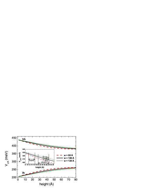
Figure 2: (color online) The top of the holes (h) potentials calculated from the strain Hamiltonian at $x$ = 0 and $y$ = 0 as function of the height of InAs/InP self-assembled CQWRs. The dashed (red), full (black), and dotted (green) curves correspond to the heavy-hole (hh) and the light-hole (lh) potentials of the CQWRs with width $w$ = 80 Å, $w$ = 100 Å and $w$ = 120 Å, respectively. The inset shows the heavy-hole band offsets for the High T (HT) and Low T (LT) samples (see Ref. Exp, ).

In Ref. Exp, the photoluminescence carrier recombination in InAs/InP self-assembled wires was reported. The PL spectra of two adjacent emission peaks of the High T (HT) and Low T (LT) samples were investigated. The HT and LT samples were grown at different substrate temperature and correspond to CQWRs with different heights. The observed energy distance between these two peaks for both the HT and LT samples correspond to 1 ML (1 ML = 3 Å) height fluctuation. The average geometric values of the CQWRs were measured by XTEMExp .

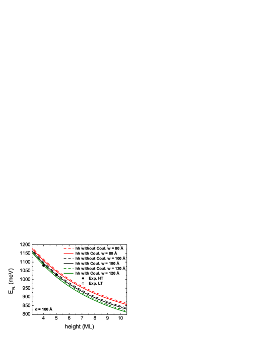
Figure 3: (color online) PL peak energies as a function of the InAs/InP CQWRs height. The full and dashed lines are the theoretical calculations for the heavy-hole excitons with and without taking into account the Coulomb interaction, respectively, for the InAs/InP CQWRs with width $w$ = 80 Å (red curves), $w$ = 100 Å (black curves) and $w$ = 120 Å (green curves). The full and open circles correspond to the experimental data for HT and LT samples, respectively.

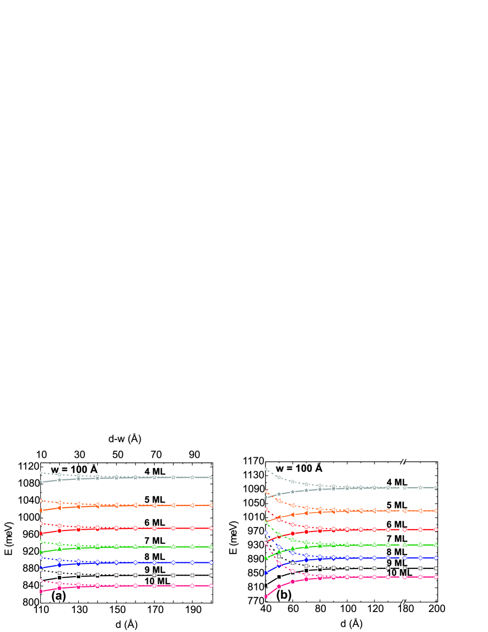
Figure 4: (color online) The heavy-hole exciton ground and the first excited state energies as a function of distance $d$ in InAs/InP horizontally [(a)] and vertically [(b)] CQWRs. The top scale, $d-w$, in the graph [(a)] is the distance between the edges of two horizontally CQWRs (see Fig. 1(a)). The full curves with the closed symbols and dashed curves with the open symbols correspond to the ground and the first excited state energies of the exciton, respectively. The curves with the stars (grey), rotated triangles (orange), circles (red), triangles (green), diamonds (blue), squares (black) and pentagons (pink) correspond to the CQWRs with the height of 4 to 10 ML (1 ML is 3 Å) in steps of 1 ML and width of 100 Å, respectively.

In order to compare our calculations with the experimental data for the HT and LT samples we consider the model of two horizontally CQWRs, as mentioned in previous section. We used the heavy- and light-hole band offsets depicted by the dashed, full, and dotted curves in the inset of Fig. 2. The different curves correspond to different widths of the CQWRs for both heavy- and light-holes. Strain splits the heavy- and light-hole bands by a value which depends on the matrix elements of the Pikus-Bir-Hamiltonian which depend on the dimension of the quantum wiremy1 . From Fig. 2 we notice that the heavy-hole curves are above the light-hole curves in the whole range of heights up to 80 Å and for three different widths: $w$ = 80 Å, $w$ = 100 Å and $w$ = 120 Å. Therefore, we conclude that the heavy-hole state is the ground state, as in the case of a strained quantum well. Further, in Fig. 3, we compare the calculated PL peak energies as a function of the height of the InAs/InP CQWRs for three different widths with the experimental PL energies of the HT and LT samples (indicated by the symbols in Fig. 3). The distance between the quantum wires is fixed to $d$ = 180 Å. We are allowed to move the experimental points along the height direction with a step of 1 ML to find the optimal agreement with the theoretical curves. The results for the Coulomb interaction included (when both electron and heavy-hole are in the ground state) fit best the experimental points (see full curves in Fig. 3), when the two peaks of the HT sample correspond to wire heights of 4 and 5 ML, and the two peaks of the LT sample correspond to heights of 9 and 10 ML. These height values of 4 and 5 ML, and the values of 9 and 10 ML agree with those from XTEM measurements, where the average value of the height for the HT was found to be $h$ = 14 $\pm$ 3 Å, for the LT $h$ = 25 $\pm$ 5 Å, and the average width was found to be $w$ = 100 $\pm$ 20 Å.

IV Inter-wire coupling: a theoretical investigation

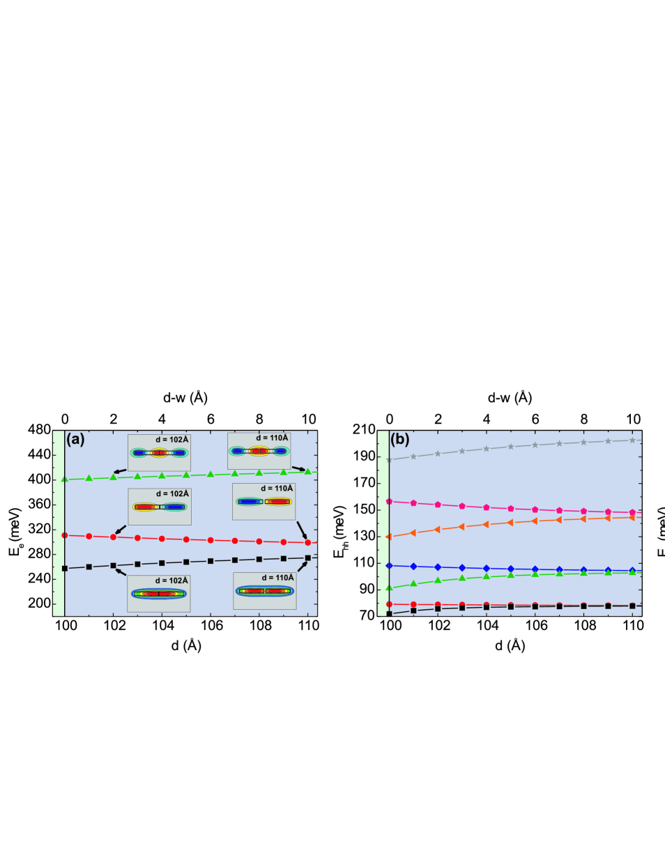
Figure 5: (color online) The energy for the electron [(a)] ground state and the next two excited states, the heavy-hole [(b)] ground state and the next six excited states and the light-hole [(c)] ground state and the next two excited states as a function of distance $d$ between the wires in InAs/InP horizontally CQWRs with height $h$ = 27 Å and width $w$ = 100 Å. The top scale, $d-w$, in the graphs [(a)], [(b)] and [(c)] is the distance between the edges of two horizontally CQWRs (see Fig. 1(a)). The insets in the graph [(a)] show the contour plots of the electron wavefunctions for $d$ equal to 102 and 110 Å.

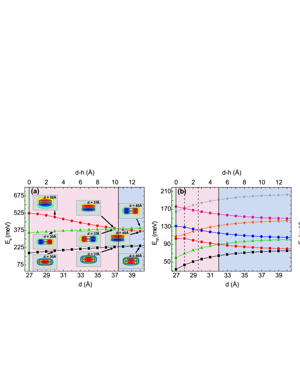
Figure 6: (color online) The same as Fig. 5 but now for vertically CQWRs. The top scale, $d-h$, in the graphs [(a)], [(b)] and [(c)] is the distance between the edges of two vertically CQWRs (see Fig. 1(b)). The insets in the graph [(a)] show the contour plots of the electron wavefunctions when $d$ is 40 Å, 37 Å and 30 Å.

Here we investigate the coupling for two wires when placed along the wire width and the wire height direction, i.e. the horizontally and vertically CQWRs (see Fig. 1). In Fig. 4 we examine the dependence of the energy of the ground and the first excited state of the heavy-hole exciton as a function of the distance between the wires. We study this dependence when the height of the wires vary from 4 up to 10 ML (the width of the wires is fixed to 100 Å), which is an experimental range of heights, as known from a previous PL studymy3 . Fig. 4(a) shows the results for the horizontally CQWRs where heavy-hole exciton ground state energy slightly decreases as the interdistance becomes smaller, while the first exciton excited state energy slowly increases, as expected. For large interdistances the energy levels become twofold degenerate. The energy of the bound state (the ground state) decreases and the energy of the anti-bounding state (the first excited state) increases due to the lifting of the degeneracy of the two-fold ground state. It is also clear that there is no evidence of coupling in InAs/InP self-assembled wires when the interdistance between the two wires is 180 Å and therefore the results presented in Fig. 3 are identical to those for a single (i.e. uncoupled) quantum wire. Coupling sets in when $d$ becomes roughly smaller than 160 Å. Similar to the horizontally CQWRs, in vertically CQWRs the heavy-hole exciton ground state (first excited state) energies decrease (increase) as $d$ diminishes (see Fig. 4(b)). Here coupling is found when $d$ is smaller than 120 Å, and a stronger dependence at small values of $d$ for the exciton ground and the first excited states is noticed.

In Figs. 5 and 6 we examine the dependence of the energy for the individual particles at smaller inter-wire distance $d$, up to the moment when two wires in the coupled wire touch each other which occurs for $d$ = 100 Å in case of the horizontally CQWRs and when $d$ = 27 Å (we consider the height $h$ to be 9 ML = 27 Å in Figs. 5 and 6) for the vertically CQWRs (see the left vertical straight lines at $d-w$ and $d-h$ equal to 0 Å in Figs. 5 and 6, respectively). Let us consider first the single particles for the horizontally CQWRs (see Figs. 5(a) - 5(c)). For all particles (electron, heavy- and light-hole) we observe a continuous energy splitting until $d$ reaches 100 Å ($d-w$ = 0 Å), and the wavefunctions simply merge into the wavefunction of a single wire (compare the wavefunctions for the electron ground and excited state energies in the inset of Fig. 5(a), when $d$ is equal to 102 and 110 Å). Besides, we can see that the energy splitting between the bound state and the anti-bounding state is larger for the electron and the light-hole (see Figs. 5(a) and 5(c)) as compared to the heavy-hole states (see Fig. 5(b)). The larger sensitivity of the electron and the light-hole to the variation of the inter-wire distance is because of their lighter effective mass which is about 10 times less in the wire and at least 5 times less in the barrier than the heavy-hole effective mass.

Interesting new effects arise when we consider vertically coupled InAs/InP quantum wires. Again, the electron ground state wavefunction merges together (compare the electron ground state wavefunction in Fig. 6(a), when $d$ equals to 40, 37 and 30 Å). Meanwhile, the ground state energy of the electron decreases with decreasing $d$, as we have previously shown in Fig. 4(b). For the first excited state energy of the electron, when the distance between the wires becomes smaller (see the curve (red) with the circles in Fig 6(a)), the electron first excited state energy increases, as it is shown in Fig. 4(b) up to a certain value of $d$ between 37 and 38 Å (see the right vertical straight line in Fig. 6(a)). Starting from this value and up to $d$ equal to $h$, it is energetically more favorable for the electron to jump to another state, whose energy decreases (see the curve (green) with the triangles in Fig. 6(a)). Also the symmetry of the electron wavefunction of the first two excited states in the transverse directions of the wires have a different behavior with variation of the inter-wire distance. For this reason there is a crossing between the excited states for the electron in the vertically coupled wires, contrary to the horizontally coupled wires where the electron wavefunction symmetry of the excited states remains the same with the varying $d$ (see Fig. 5(a) and Fig. 6(a)). Furthermore, in the inset of Fig. 6(a), where the contour plots of the electron wavefunctions are shown, before and after the crossing the symmetry with respect to the nodal line changes for the first excited state and in the opposite way for the second excited state. Note that when $d$ is between 27 and roughly 38 Å, the wavefunction for the first two excited states has the same character as for a rectangular single wire. A similar crossing for the heavy-hole (see the right vertical straight line in Fig 6(b) when $d$ equals 32 Å) and for the light-hole (see the right vertical straight line in Fig 6(c) when $d$ is roughly 37 Å) between the first and second excited states is observed. Besides, for the heavy-hole we found crossings between the fourth and fifth (see the dashed vertical line between 29 and 30 Å) as well as between the sixth and seventh (see the dashed vertical line placed at $d$ = 28 Å) heavy-hole excited states. The electron and the light-hole have only three bound states. Note that for electron and holes in InAs/InP vertically CQWRs three regions can be distinguished:

(1) coupled region where the wavefunctions of the lowest levels behave as for a single rectangular wire. But energetically they are already in the coupled regime because the levels are all split (see the middle region in Figs. 6(a) and 6(c));

(2) coupled region where the energies and the densities of the lowest levels behave as for the coupled wires (see the right region in Figs. 6(a) and 6(c));

(3) decoupled region, where all levels are twofold degenerate (when $d$ is large).

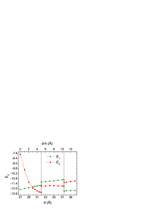
Figure 7: (color online) The electron-heavy-hole Coulomb interaction energy as a function of distance $d$ between the wires in InAs/InP vertically CQWRs with height $h$ = 27 Å and width $w$ = 100 Å. The curves with the triangles (green) and circles (red) correspond to the Coulomb interaction energy between the particles in the first and second excited state, respectively. The top scale, $d-h$, in the graphs is the distance between the edges of two vertically CQWRs (see Fig. 1(b)).

Next, we investigate the electron-hole Coulomb interaction energy dependence on the distance $d$ between two vertically CQWRs. In order to calculate the Coulomb energy of the first (second) excited state we solve the 1D Schrödinger equation for the relative exciton motion in the $z$-direction (see Eq. (5)) with the effective potential of the first (second) excited state

$$U_{eff1(2)}(z) = \int\ dx_{e}dy_{e}dx_{h}dy_{h}|\Psi_{1(2)e}|^{2}|\Psi_{1(2)h}|^{2}\times$$ (8)

$$\left(-\frac{e^{2}}{\varepsilon|\mathbf{r}_{e}-\mathbf{r}_{h}|}\right),$$

where $\Psi_{1(2)}$ is the electron and hole wavefunction of the first (second) excited state. In Fig. 7 the Coulomb energies between the electron and heavy-hole both in the first excited state (see the curve with the triangles in Fig. 7) and in the second excited state (see the curve with the circles in Fig. 7) are shown. We found abrupt jumps for these two energies at the crossing of the first two excited states for the electron at $d$ = 37.4 Å and the heavy-hole $d$ = 32 Å. Both energies decrease continuously up to the crossing of the excited states of the electron (see the right vertical line at 37.4 Å in Fig. 7), meanwhile the absolute value of the Coulomb energy E₁ is larger than the absolute value of the Coulomb energy E₂ of the second excited state. After this crossing up to $d$ = 32 Å the situation is opposite, i.e., $|$E₂$|$ $>$ $|$E₁$|$ even when the symmetry of the heavy-hole wavefunctions of the first two excited states does not change (it changes at $d$ = 32 Å). This means a larger electron contribution to the Coulomb interaction energy of the excited states in comparison to the heavy-hole one. When the crossing point of the heavy-hole excited states is reached (see the left vertical line), the second abrupt jump in the Coulomb energy is observed. However, because of the spill-over of the electron wavefunction of the second excited state (there is no spill-over effect observed for the heavy-hole excited states), the absolute value of the Coulomb energy E₂ decreases after this crossing. Therefore, the Coulomb energy E₂ becomes smaller in absolute value than the value of E₁ for $d$ $<$ 30 Å. Close and at the crossing points, i.e. $d$ $=$ 32 Å and 37.4 Å, there will be a strong Coulomb interaction induced mixing of the energy levels which should be included. For this reason we took the electron (hole) wavefunction as a linear combination of the first and the second excited state wavefunction

$$\Psi_{e(h)}=(a\Psi_{1e(h)}+\Psi_{2e(h)})/\sqrt{1+|a|^{2}},$$ (9)

where ’a’ is a weighting parameter which is taken as a variational coefficient that minimizes the total exciton energy. In Fig. 8 we plot the exciton energy dependence of the first two excited states on the inter-wire distance $d$ between two vertically aligned CQWRs. The results of the two different methods are presented: by solving the single-particle Schrödinger equations; and by using the variational technique. In the first one, as was already mentioned in Sect. II, the wavefunction in the $xy$-plane for the first (second) excited state of the exciton is assumed as the product of the wavefunction of the electron and the heavy-hole in the first (second) excited state. Then, the total exciton energy of the first (second) excited state equals $E_{Exc.,1(2)}$ = $E_{e,1(2)}$+$E_{hh,1(2)}$+$E_{c,1(2)}$. In the second approach, the total exciton wavefunction in the $xy$-direction is taken as

$$\Psi(x_{e},y_{e},x_{h},y_{h},a,b)=\Psi_{e}(x_{e},y_{e},a)\Psi_{h}(x_{h},y_{h},b),$$ (10)

using the new wavefunctions (see Eq. (9)). Then, we average the kinetic part and the Coulomb interaction part in the exciton Hamiltonian (see Eq. (1)). After this averaging we obtain the 1D Schrödinger equation for the relative exciton motion in the $z$-direction, where the single particle energies $E_{e}$ + $E_{hh}$ are now replaced by $|a|^{2}$$E_{e,1}$+$E_{e,2}$+$|b|^{2}$$E_{hh,1}$+$E_{hh,2}$ and the effective potential becomes now

$$U_{eff}(z,a,b) = N\int dx_{e}dy_{e}dx_{h}dy_{hh}(|a|^{2}|b|^{2}|\Psi_{1e}|^{2}|\Psi_{1h}|^{2}$$ (11)

$$+|a|^{2}|\Psi_{1e}|^{2}|\Psi_{2h}|^{2}+|b|^{2}|\Psi_{2e}|^{2}|\Psi_{1h}|^{2}$$

$$+|\Psi_{2e}|^{2}|\Psi_{2h}|^{2})\times\left(-\frac{e^{2}}{\varepsilon|\mathbf{r}_{e}-\mathbf{r}_{h}|}\right),$$

where $N=1/((1+|a|^{2})(1+|b|^{2}))$. By numerically integrating this equation and by minimizing the total energy we obtain the exciton energy. From Fig. 8 we notice an anti-crossing for the exciton excited state energies at $d$ = 37.4 Å, where the crossing of the first two excited states for the electron was found. However, at the point $d$ = 32 Å both energies slightly change their behavior. The slope of the curves of these exciton energies change insignificantly (see the curves E₁ and E₂ near $d$ = 32 Å in Fig. 8). Hence, the crossing of the electron first and the second excited state energies leads to the anti-crossing of the exciton first and the second excited state energies, but the crossing of the heavy-hole first two excited states does not affect much the exciton excited state energies. Moreover, we see full agreement in the whole inter-wire region $d$ between the energy calculated by the variational method and between the first excited state energy of the exciton. It is expected, since we always get the first excited state energy of the exciton after minimization of the electron and heavy-hole terms with the first and second excited state energies, and the terms with the Coulomb interaction energy. However, near the crossing of the excited states of the electron and the heavy-hole, the exciton first excited state energy differs by less than 2 meV from the one calculated from the variational technique (see the insets (a) and (b) of Fig. 8). At the crossing points there are abrupt jumps for the curve E₁, resulting from the jump in the Coulomb interaction energy for the first excited state (see Fig. 7), while continuous behavior is found for the variational calculation results (see the curve with the open squares in the insets of Fig. 8). This is because near these crossings the difference between the energies of the excited states of the electron and the heavy-hole becomes smaller than the difference between the Coulomb interaction energies of the excited states.

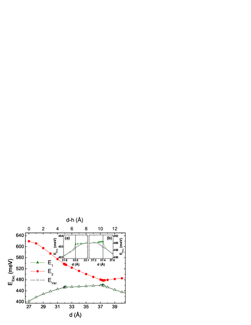
Figure 8: (color online) The heavy-hole exciton energy as a function of distance $d$ between the wires in InAs/InP vertically CQWRs with height $h$ = 27 Å and width $w$ = 100 Å. The curves with the full triangles (green) and full circles (red) correspond to the exciton first and second excited state energies, respectively. The curve with the open squares (black) correspond to our variational calculation. The top scale, $d-h$, in the graphs is the distance between the edges of the two vertically CQWRs. The inset shows the exciton energy near the crossing of the first and the second excited states for heavy-hole (a) and electron (b)(see Figs. 6(a) and 6(b)).

V Conclusions

We investigated the coupling in InAs/InP horizontally and vertically CQWRs. The calculation are performed within the single-band effective mass approximation. The strain effect on the band offsets, the mass mismatch in the barrier and the wire, and the Coulomb interaction between the electron-hole pair are included. We found that the heavy-hole state is the ground state.

The PL energy for horizontally coupled InAs/InP wires was calculated as function of the wire height at fixed width. From comparison with the observed PL energies we derive the height of the quantum wire which is in good agreement with those from the experimental XTEM measurements. No inter-wire coupling of the exciton in the experimentally grown InAs/InP self-assembled quantum wires with period $d$ = 180 Å was found. Such coupling effects is predicted to show up when the distance $d$ between the wires is smaller than 160 Å.

Numerical results for InAs/InP horizontally coupled system show one coupling regime for all inter-wire distances between the wires. However, for vertically CQWRs a crossing between the excited states for the particles is predicted when the distance between the wires approaches the value of the wires heights. Due to this crossing two coupling regimes for InAs/InP vertically CQWRs are found. In the first coupling regime the electron, heavy- and light-hole densities for the lowest levels have the same behavior as in a single square wire, while in the second coupling regime both the energies and densities for the lowest levels act as in ordinary coupled wires.

Anti-crossing for exciton excited state energies in vertically CQWRs is predicted for the inter-wire distance where the crossing of the first and the second excited states for the electron is found. Exciton excited state energies are slightly affected when the symmetry of the wavefunction of heavy-hole excited states in vertically CQWRs changes. In a PL experiment the heavy-hole exciton line is bright while the corresponding one for the light-hole is dark due to a selection rule. Therefore, we did not present results for the light-hole exciton.

VI Acknowledgments

This work was supported by the European Commission network of excellence: SANDiE and the Flemish Science Foundation (FWO-Vl). The authors thank M. Hayne and V. V. Moshchalkov for stimulating discussions.

References

- (1) L. Esaki and R. Tsu, IBM J. Res. Dev. 14, 61 (1970).
- (2) See, for example, IEEE J. Quantum Electron. QE-22, 1609 (1986).
- (3) R. Tsu and G. Döhler, Phys. Rev. B 12, 680 (1975).
- (4) S. L. Chuang and B. Do, J. Appl. Phys. 62, 1290 (1987).
- (5) T. Weil and B. Vinter, J. Appl. Phys. 60, 3227 (1986).
- (6) K. Kern, D. Heitmann, R. R. Gerhardts, P. Grambow, Y. H. Zhang, and K. Ploog, Phys. Rev. B 44, 1139 (1991).
- (7) H. Weman, M. Potemski, M. E. Lazzouni, M. S. Miller, and J. L. Merz, Phys. Rev. B 53, 6959 (1996).
- (8) H. Weman, D. Y. Oberli, M. A. Dupertuis, F. Reinhardt, A. Gustafsson, and E. Kapon, Phys. Rev. B 58, 1150 (1998).
- (9) H. X. Li, J. Wu, Z. G. Wang, and T. Daniels-Race, Appl. Phys. Lett. 75, 1173 (1999).
- (10) W. Ma, R. Nötzel, A. Trampert, M. Ramsteiner, H. Zhu, H.-P. Schönherr, and K. H. Ploog, Appl. Phys. Lett. 78, 1297 (2001).
- (11) K. F. Karlsson, H. Weman, M.-A. Dupertuis, K. Leifer, A. Rudra, and E. Kapon, Phys. Rev. B 70, 045302 (2004).
- (12) C. Pryor, Phys. Rev. Lett. 80, 3579 (1998).
- (13) B. Szafran, S. Bednarek, and J. Adamowski, Phys. Rev. B 64, 125301 (2001).
- (14) I. Shtrichman, C. Metzner, B. D. Gerardot, W. V. Schoenfeld, and P. M. Petroff, Phys. Rev. B 65, 081303(R) (2002).
- (15) K. L. Janssens, B. Partoens, and F. M. Peeters, Phys. Rev. B 66, 075314 (2002).
- (16) Y. B. Lyanda-Geller, T. L. Reinecke, and M. Bayer, Phys. Rev. B 69, 161308(R) (2004).
- (17) J.-L. Zhu, W. Chu, Z. Dai, and D. Xu, Phys. Rev. B 72, 165346 (2005).
- (18) L. González, J. M. García, R. García, F. Briones, J. Martínez-Pastor, and C. Ballesteros, Appl. Phys. Lett. 76, 1104 (2000).
- (19) B. Alén, J. Martínez-Pastor, A. García-Cristobal, L. González, and J. M. García, Appl. Phys. Lett. 78, 4025 (2001).
- (20) D. Fuster, L. González, Y. González, J. Martínez-Pastor, T. Ben, A. Ponce, and S. I. Molina, Eur. Phys. J. B 40, 433 (2004).
- (21) Y. Sidor, B. Partoens, and F. M. Peeters, Phys. Rev. B 71, 165323 (2005).
- (22) Y. Sidor, B. Partoens, F. M. Peeters, N. Schildermans, M. Hayne, V. V. Moshchalkov, A. Rastelli, and O. G. Schmidt, Phys. Rev. B 73, 155334 (2006).
- (23) I. Vurgaftman, J. R. Meyer, and L. R. Ram-Mohan, J. Appl. Phys. 89, 5815 (2001).
- (24) J. Maes, M. Hayne, Y. Sidor, B. Partoens, F. M. Peeters, Y. González, L. González, D. Fuster, J. M. García, and V. V. Moshchalkov, Phys. Rev. B 70, 155311 (2004).