Differential Geometry of Polymer Models: Worm-like Chains, Ribbons and Fourier Knots

Abstract

We analyze several continuum models of polymers: worm-like chains, ribbons and Fourier knots. We show that the torsion of worm-like chains diverges and conclude that such chains can not be described by the Frenet-Serret (FS) equation of space curves. While the same holds for ribbons as well, their rate of twist is finite and, therefore, they can be described by the generalized FS equation of stripes. Finally, Fourier knots have finite curvature and torsion and, therefore, are sufficiently smooth to be described by the FS equation of space curves.

I Introduction

Recent progress in the ability to manipulate single biomolecules such as double stranded DNA and protein filaments Bensimon , prompted the development of continuum models of complex polymers capable of describing bending fluctuations and finite extensibility under tension (extensions of the worm-like chain model Marko ) as well as models that can describe twist rigidity, spontaneous twist and chiral response to torque (the ribbon model rabin ). These models are defined by their elastic energy functions which are then used to generate the equilibrium ensemble of polymer conformations, based on the conventional Gibbs distribution approach (i.e., weighting the conformations by an appropriate Boltzmann factor). While this approach proved to be quite successful for open polymers mezard ; yevgeny , it could not be applied to generate the conformations of polymer loops and to study properties of circular double stranded DNA such as supercoiling and formation of knots. In order to cope with the latter problem, we developed a purely mathematical procedure of generating closed curves, based on the expansion of the components of the polymer conformation vector $\vec{r}(t)$ ($t$ is some parametrization of the contour of the loop) in finite Fourier series and taking the corresponding Fourier coefficients from some random distribution Shay2 . We found that this distribution of Fourier knots could be fine tuned to mimic some of the large scale properties of closed Gaussian loops and small scale properties of worm-like chain, this could not be achieved using a single persistence length.

The present deals attempts to establish a common framework for the discussion of the above physical and mathematical models of polymers, by classifying them according to their smoothness. A continuous curve $\vec{r}(s)$ ($s$ is the contour parameter which measures the distance along the contour) is defined as an $m$-smooth curve if its $m$th derivative $d^{m}\vec{r}/ds^{m}$ is a continuous function of $s$. In section II we introduce the fundamental equations of differential geometry of space curves and of stripes and show that these equations describe space curves that are at least $2$-smooth and stripes that are at least $1$-smooth. This is equivalent to saying that while such space curves must have finite torsion, stripes must have finite rate of twist but their torsion is free to take any value along their contour. In section III we show that worm-like chains belong to the class of freely rotating models, with uniformly distributed dihedral angles, divergent torsion and a normal whose direction jumps discontinuously as one moves along the contour of the chain and, therefore, such objects can not be described by the Frenet-Serret (FS) equation. We also show that because the energy of  a ribbon depends on its twist, the typical conformations of  ribbons have finite rate of twist but their torsion diverges at many points along the contour.  In section IV we compare the ensembles of $1$-smooth (ribbons) and $\infty$-smooth (Fourier knots) curves and show that typical realizations of the latter (but not the former) ensemble, have finite torsion and a smoothly varying normal and can be described by the FS equation. We also calculate the distributions of spatial distances between two points on the contour of the curve in the above ensembles and find that these distributions differ significantly only for distances of the order of persistence length. Finally, in section V we discuss our results and conclude that unlike worm-like chains and ribbons which possess no torsional rigidity, the ensemble of curves generated by the Fourier knot algorithm can be characterized by finite torsional persistence length.

II Differential geometry of curves and stripes

It is often convenient to represent a space curve $\vec{r}(s)$ defined in a space-fixed coordinate frame by intrinsic coordinates, as follows. At every point along the curve ($0\leq s\leq L$) one constructs a set of three orthogonal unit vectors known as the Frenet frame: the tangent $\hat{t}$ defined as $\hat{t}(s)=d\vec{r}/ds$, the normal $\hat{n}(s)$ which points in the direction of $d\hat{t}/ds$ and the binormal $\hat{b}(s)=\hat{t}(s)\times\hat{n}(s)$. The rotation of the Frenet frame as one moves along the contour of the curve is described by the Frenet-Serret (FS) equation willmore :

$$\frac{d}{ds}\left(\begin{array}[]{c}\hat{t}\\ \hat{n}\\ \hat{b}\end{array}\right)=\left(\begin{array}[]{ccc}0&\kappa&0\\ -\kappa&0&\tau\\ 0&-\tau&0\end{array}\right)\left(\begin{array}[]{c}\hat{t}\\ \hat{n}\\ \hat{b}\end{array}\right)$$ (1)

where $\kappa$ is the curvature and $\tau$ is the torsion (in general, both are functions of $s$). The condition of validity of the above equation is that $\kappa ds,\tau ds\rightarrow 0$ as $ds\rightarrow 0$ everywhere along the curve. It is straightforward to show that

$$\kappa(s)=\left|\frac{d^{2}\vec{r}}{ds^{2}}\right|,\qquad\tau(s)=\frac{d\vec{r}}{ds}\cdot\left(\frac{d^{2}\vec{r}}{ds^{2}}\times\frac{d^{3}\vec{r}}{ds^{3}}\right)\left|\frac{d^{2}\vec{r}}{ds^{2}}\right|^{-2}$$ (2)

and we conclude that since the condition of validity of the FS equation is that the torsion is finite everywhere along the curve, the curve should be at least $2$-smooth.

Given the curvature and the torsion at each point along the curve, one can solve Eq. (1), calculate the tangent $\hat{t}(s)$ and integrate it to construct the parametric representation of the space curve, $\vec{r}(s)$. The above construction is unique in the sense that any pair of functions $\kappa(s)$ and $\tau(s)$ defined on the interval $0<s<L$, can be uniquely mapped to a space curve $\vec{r}(s)$ of length $L$. The simplest examples are (a) $\kappa=const.,\tau=0$ which yields a planar circle of radius $\kappa^{-1}$ and (b) $\kappa=const.,\tau=const.$ which corresponds to a helix.

We now turn to consider stripes of length $L$, width $W$ (such that $L\gg W$ ) and thickness $D\rightarrow 0$. Unlike a space curve which is uniquely defined by the tangent vector $\hat{t}(s)$ (the normal and the binormal are auxiliary constructs, needed only to calculate the tangent, given the curvature and the torsion), a stripe is a slice of a plane with which one can associate two orthogonal unit vectors $\hat{t}_{1}$ (in plane) and $\hat{t}_{2}$ (normal to the plane). The spatial configuration of the stripe is thus defined by the local orientation (at each point $s$ on the centerline) of the orthogonal triad known as the Darboux frame which specifies the directions of the two axes $\hat{t}_{1}$ and $\hat{t}_{2}\,$ and that of the tangent to the centerline that runs along the long axis of the stripe, $\hat{t}\equiv\hat{t}_{3}$. While a space curve is completely defined by the two functions $\kappa(s)$ and $\tau(s)$, a stripe is represented by three generalized curvatures $\omega_{k}(s)$ ($k=1,2,3$) that determine the unit vectors $\left\{\hat{t}_{i}\right\}$ via the generalized Frenet-Serret equation SolidShape ,

$$\frac{d}{ds}\left(\begin{array}[]{c}\hat{t}_{3}\\ \hat{t}_{1}\\ \hat{t}_{2}\end{array}\right)=\left(\begin{array}[]{ccc}0&\omega_{2}&-\omega_{1}\\ -\omega_{2}&0&\omega_{3}\\ \omega_{1}&-\omega_{3}&0\end{array}\right)\left(\begin{array}[]{c}\hat{t}_{3}\\ \hat{t}_{1}\\ \hat{t}_{2}\end{array}\right).$$ (3)

This can be written compactly as $\dot{\hat{t}}_{i}=A_{ik}\hat{t}_{k}$ where $A_{ik}=-\epsilon_{ijk}\omega_{j}$ ($\epsilon_{ijk}$ is the Levi-Civita tensor). Inspection of Eq. (3) shows that $\omega_{i}(s)ds$ is the infinitesimal angle of rotation about the direction $\hat{t}_{i}(s)$ and the condition of validity of the generalized FS equation is that this angle vanishes in the limit $ds\rightarrow 0$. However, unlike the torsion $\tau\,$ which is completely determined by the space curve $\vec{r}(s)$ and can be expressed in terms of its first three derivatives, the rate of twist $\omega_{3}$ is the local rate (per unit length) of rotation about the tangent to this curve and, as such, it depends only on the orientation of $\hat{t_{1}}$ and $\hat{t_{2}},$ and can not be expressed in terms of the centerline $\vec{r}(s)$ and its derivatives! We conclude that in order for Eq. (3) to hold, the centerline of the stripe should be represented by a $1$-smooth curve.

Since both couples of unit vectors $\left\{\hat{n},\hat{b}\right\}$ and $\left\{\hat{t}_{1},\hat{t}_{2}\right\}$ lie in the plane perpendicular to the local tangent, the triads $\left\{\hat{t},\hat{n},\hat{b}\right\}$ and $\left\{\hat{t_{3}},\hat{t}_{1},\hat{t}_{2}\right\}$ are connected by

$$\left(\begin{array}[]{c}\hat{t}_{3}\\ \hat{t}_{1}\\ \hat{t}_{2}\end{array}\right)=\overleftrightarrow{S}\left(\begin{array}[]{c}\hat{t}\\ \hat{n}\\ \hat{b}\end{array}\right)$$ (4)

where the matrix

$$\overleftrightarrow{S}=\left(\begin{array}[]{ccc}1&0&0\\ 0&\cos\alpha&\sin\alpha\\ 0&-\sin\alpha&\cos\alpha\end{array}\right)$$ (5)

generates a rotation by an angle $\alpha$ about the $\hat{t}=\hat{t}_{3}$ axis. Assuming that the centerline of the stripe can be represented by the FS equation (i.e., that it is an $2$-smooth curve), one can express the generalized FS equation in terms of the curvature, torsion and the angle $\alpha$ between the directions of the binormal $\hat{b}$ and the $\hat{t_{1}}$ axis:

$$\frac{d}{ds}\left(\begin{array}[]{c}\hat{t}_{3}\\ \hat{t}_{1}\\ \hat{t}_{2}\end{array}\right)=\left(\begin{array}[]{ccc}0&\kappa\cos\alpha&-\kappa\sin\alpha\\ -\kappa\cos\alpha&0&\dfrac{d\alpha}{ds}+\tau\\ \kappa\sin\alpha&-\dfrac{d\alpha}{ds}-\tau&0\end{array}\right)\left(\begin{array}[]{c}\hat{t}_{3}\\ \hat{t}_{1}\\ \hat{t}_{2}\end{array}\right).$$ (6)

Comparing (6) with (3) yields:

$$\begin{array}[]{c}\omega_{1}=\kappa\sin(\alpha)\\ \omega_{2}=\kappa\cos(\alpha)\\ \omega_{3}=d\alpha/ds+\tau\end{array}$$ (7)

Conversely,

$$\kappa=\sqrt{\omega_{1}^{2}+\omega_{2}^{2}}$$ (8)

$$d\alpha/ds=\frac{\omega_{2}\left(d\omega_{1}/ds\right)-\omega_{1}\left(d\omega_{2}/ds\right)}{\omega_{1}^{2}+\omega_{2}^{2}}$$ (9)

$$\tau=\omega_{3}-d\alpha/ds$$ (10)

However, since the centerline of the stripe is required to be only $1$ -smooth, these relations do not hold in general!

III Polymer models: Worm-like Chains and Ribbons

Physical models of polymers are based on the choice of a geometrical model and an energy functional. The simplest and the most prevalent model is that of a continuous Gaussian random walk, with which one can associate a free energy that describes the entropic cost of stretching the polymer chain, $E_{GRW}=\frac{1}{2}ak_{B}T\int\nolimits_{0}^{L}{dt}\left({d}\vec{{r}}{/dt}\right)^{2}.$ Here $a$ is the “monomer” (cutoff) length, $k_{B}$ is the Boltzmann constant and $T$ is the temperature colby . Notice that this free energy is expressed only in terms of the first derivative of the trajectory, ${d\vec{{r}}/dt}$ and, therefore, space curves that describe polymer conformations in the continuous Gaussian random walk model have to be only $0$-smooth (only the curve itself and not its derivatives, has to be continuous everywhere).
The worm-like chain model of polymers combines bending elasticity and inextensibility (the latter condition can be expressed as $\left|{d\vec{{r}}/ds}\right|=1$) and, assuming that the stress-free state corresponds to a straight line, the energy can be written as Kamien

$$E_{WLC}=\frac{1}{2}b\int\nolimits_{0}^{L}{ds(\kappa(s))^{2}=}\frac{1}{2}b\int\nolimits_{0}^{L}{ds(d\hat{t}/ds)^{2}}.$$ (11)

Since the energy depends only on the curvature ${\kappa}$ and does not depend on the torsion $\tau,$ the corresponding space curve has only $1$ -smooth. Note that curves described by the FS equations have to be at least $2$-smooth and, therefore, worm-like chains are not sufficiently smooth to be described by the fundamental equations of differential geometry of space curves! In order to get physical intuition about the origin of the problem, lets consider a discretized model of a continuous curve in which the polymer is made up of connected straight segments of length $\Delta s$ each, such that the direction of the segment at point $s$ is given by the tangent to the original chain at this point, $\hat{t}(s)$ (the continuum limit is recovered as $\Delta s\rightarrow 0$). The angle between neighboring segments is denoted as $\Delta\theta(s)$ and, in order to describe the non-planar character of a general space curve, one has to introduce the dihedral angle $\Delta\varphi(s)$ between the two successive planes $\left\{\hat{t}(s),\hat{t}(s+\Delta s)\right\}$ and $\left\{\hat{t}(s+\Delta s),\hat{t}(s+2\Delta s)\right\}$ determined by three successive segments at points $s,$ $s+\Delta s$ and $s+2\Delta s$. Since $\Delta\varphi(s)$ is also the angle between neighboring binormals $\hat{b}(s)$ and $\hat{b}(s+\Delta s)$, the Frenet frames at points $s$ and $s+\Delta s$ are related by a simple rotation

$$\left(\begin{array}[]{c}\hat{t}(s+\Delta s)\\ \hat{n}(s+\Delta s)\\ \hat{b}(s+\Delta s)\end{array}\right)=\overleftrightarrow{B}(s)\left(\begin{array}[]{c}\hat{t}(s)\\ \hat{n}(s)\\ \hat{b}(s)\end{array}\right)$$ (12)

where the rotation matrix $\overleftrightarrow{B}(s)$ is given by

$$\overleftrightarrow{B}(s)=\left(\begin{array}[]{ccc}\cos\Delta\theta&\sin\Delta\theta&0\\ -\cos\Delta\varphi\sin\Delta\theta&\cos\Delta\varphi\cos\Delta\theta&\sin\Delta\varphi\\ \sin\Delta\varphi\sin\Delta\theta&-\sin\Delta\varphi\cos\Delta\theta&\cos\Delta\varphi\end{array}\right)$$ (13)

Notice that no assumption is made so far about the magnitude of the angles $\Delta\theta$ and $\Delta\varphi$. Defining $\Delta\hat{t}(s)=\hat{t}(s+\Delta s)-\hat{t}(s),$ $\Delta$ $\hat{n}(s)=\hat{n}(s+\Delta s)-\hat{n}(s)$ and $\Delta\hat{b}(s)=\hat{b}(s+\Delta s)-\hat{b}(s)$ and subtracting the vector $(\hat{t},\hat{n},\hat{b})$ from both sides of Eq. (13),  yields

$$\left(\begin{array}[]{c}\Delta\hat{t}\\ \Delta\hat{n}\\ \Delta\hat{b}\end{array}\right)=\left(\overleftrightarrow{B}(s)-\overleftrightarrow{I}\right)\left(\begin{array}[]{c}\hat{t}(s)\\ \hat{n}(s)\\ \hat{b}(s)\end{array}\right)$$ (14)

with $\overleftrightarrow{I}$ the unit matrix. Notice that unlike the FS equation which is valid only for infinitesimal rotations of the Frenet frame, Eq. (14) describes finite rotations; the FS equation can be derived from it by dividing both sides of the equation by $\Delta s$ and taking the limit $\Delta s\rightarrow 0$ ($\underset{\Delta s\rightarrow 0}{\lim}\Delta\hat{t}/\Delta s=d\hat{t}/ds$, etc.). In order for the right hand side of Eq. (14) to remain finite in this limit, all the elements of $\overleftrightarrow{B}(s)-\overleftrightarrow{I}$ have to vanish .Since this is equivalent to the condition $\Delta\theta,$ $\Delta\varphi\ll 1$ , one can expand the cosine and sine functions in Eq. ( 13) and, upon substituting the result into Eq. (14), one recovers the FS equation with $\kappa=\lim\limits_{\Delta s\rightarrow 0}\Delta\theta/\Delta s$ and $\tau=\lim\limits_{\Delta s\rightarrow 0}\Delta\varphi/\Delta s.$

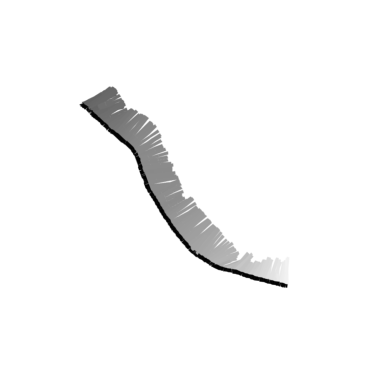
(a)(b)

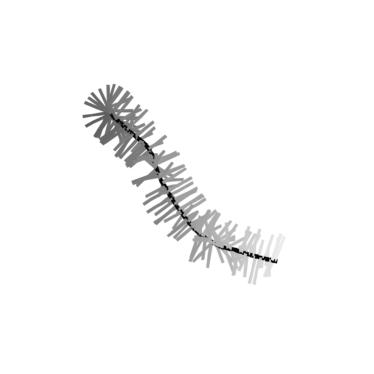
Figure 1: A typical conformation of a ribbon: the centerline is shown by the dark solid curve and the gray lines orthogonal to it show the direction of (a) one of the symmetry axes of the cross section $\hat{t}_{1}$ and (b) the normal $\hat{n}$

Returning to the worm-like chain model, we notice that while the bending energy ensures that the curvature is finite and the angle $\Delta\theta$ is always small, there is no corresponding physical restriction on the magnitude of $\Delta\varphi$ and we conclude that the worm-like chain corresponds to the class of freely rotating chain models in which the angle $\Delta\varphi$ can attain any value in the interval $\left[-\pi,\pi\right]$ . For such models, the expansion of $\overleftrightarrow{B}(s)-\overleftrightarrow{I}$ in terms of $\Delta\varphi$ breaks down and the corresponding ($1$-smooth) curves can not be described by the FS equation. Notice that if one keeps the definition $\tau=\lim\limits_{\Delta s\rightarrow 0}\Delta\varphi/\Delta s,$ the torsion can diverge at any point along the curve, generating abrupt jumps of the normal (see Fig. 1 b). Nevertheless, since the shape of a curve is completely characterized by (and only by) the tangent to it and since the latter changes continuously even for $1$-smooth curves, such a curve appears (to the eye) to be just as smooth as an $\infty$-smooth one.

Let us now consider the ribbon model of polymers which was designed to take into account rigidity with respect to twist and spontaneous twist of complex polymers such as double stranded DNA. In general, the ribbon has an asymmetric cross section with symmetry axes $\hat{t_{1}}$ and $\hat{t_{2}}$ and a centerline described by the tangent, $\hat{t_{3}}$, such that the triad of unit vectors $\left\{\hat{t_{i}}(s)\right\}\$can be associated with the Darboux frame familiar from the differential geometry of stripes. In the framework of the linear theory of elasticity of slender rods Love ), the energy of a particular configuration of a ribbon is a quadratic functional of the deviations of its three curvatures $\left\{\omega_{i}(s)\right\}$ from their equilibrium values in the stress-free state, $\left\{\omega_{0i}(s)\right\}$ rabin :

$$\begin{array}[]{c}E_{R}=\frac{1}{2}\int\nolimits_{0}^{L}ds\left[b_{1}\left(\omega_{1}-\omega_{01}\right)^{2}+b_{2}\left(\omega_{2}-\omega_{02}\right)^{2}\right.\\ +\left.b_{3}\left(\omega_{3}-\omega_{03}\right)^{2}\right]\end{array}$$ (15)

Here $b_{1}$ and $b_{2}$ are the bending rigidities associated with the two principal symmetry axes of the cross section and $b_{3}$ is the twist rigidity (the persistence lengths $\left\{a_{i}\right\}$ are obtained by dividing the corresponding rigidities by $k_{B}T$). For ribbons with a symmetric cross-section ($b_{1}=b_{2}$) and without spontaneous curvature and twist ($\omega_{0i}=0$), the above expression can be simplified

$$E_{R}=\frac{1}{2}\int\nolimits_{0}^{L}ds\left(b_{1}\kappa^{2}+b_{3}\omega_{3}^{2}\right)$$ (16)

where $\kappa^{2}=$ $\omega_{1}^{2}+\omega_{2}^{2}$. Since the above energy functional depends only on the second derivatives of the curve (curvature) and on the twist, and does not explicitly depend on the third derivatives (torsion), the torsion of the curve is not controlled by the elastic energy and, therefore, the centerline of the ribbon can not be described by the FS equation. To demonstrate it, we rewrite Eq.(3) in a discretized form, using (13) and the relation (5):

$$\left(\begin{array}[]{c}\Delta\hat{t_{3}}\\ \Delta\hat{t_{1}}\\ \Delta\hat{t_{2}}\end{array}\right)=\left(\overleftrightarrow{S}(s+\Delta s)\overleftrightarrow{B}(s)\overleftrightarrow{S}^{-1}(s)-\overleftrightarrow{I}\right)\left(\begin{array}[]{c}\hat{t_{3}}\\ \hat{t_{1}}\\ \hat{t_{2}}\end{array}\right).$$ (17)

Comparing (17) to (3) gives, in the limit $\Delta s\rightarrow 0$:

$$\begin{array}[]{c}\omega_{3}=\Delta\alpha/\Delta s+\Delta\varphi/\Delta s\rightarrow d\alpha/ds+\tau\\ \omega_{1}=\left(\Delta\theta/\Delta s\right)\sin(\alpha)\rightarrow\kappa\sin\alpha\\ \omega_{2}=\left(\Delta\theta/\Delta s\right)\cos(\alpha)\rightarrow\kappa\cos\alpha\end{array}$$ (18)

The fact that the elastic energy of a ribbon introduces a penalty for bending and twist deformations, ensures that only configurations with $\omega_{i}\Delta s\rightarrow 0$ ($i=1,2,3$) contribute in the continuum limit $\Delta s\rightarrow 0$ and, therefore, the conformations of a ribbon can be described by the generalized FS equation ( 3). Inspection of Eq. (18) shows that the condition that the twist accumulated over a contour distance $\Delta s,$ is small, can be expressed as $\Delta\alpha+\Delta\varphi<<1$. Since there is nothing that restricts the magnitudes of $\Delta\alpha$ and of $\Delta\varphi$ separately, they can be arbitrarily large provided that the condition $\Delta\alpha\simeq-\Delta\varphi$ is satisfied and, therefore, the torsion associated with the centerline of the ribbon can be arbitrarily large (recall that the torsion is defined as the limit of $\Delta\varphi/\Delta s$ as $\Delta s\rightarrow 0$). Indeed, inspection of a typical conformation of a ribbon (taken from the ensemble of conformations generated using the algorithm described in ref. yevgeny ) shows that even though the rate of rotation of the physical axis $\hat{t_{1}}$ is everywhere finite (Fig. 1a), the rate of rotation of the normal $\hat{n}$ is not (Fig. 1b)!

IV Ensembles of $1$-smooth and $\infty$-smooth Curves

Increasing the degree of smoothness from $m$ to $m+1$ acts as a constraint that prohibits certain configurations of a curve, and it is interesting to compare the properties of curves with different degrees of smoothness. Such a comparison is meaningful only in a statistical sense and in the following we will consider some physically relevant statistical properties of worm-like chains for which analytical results are available, with those of computer generated ensembles of ribbons ($1$-smooth) and Fourier knots ($\infty$-smooth). In order to generate the ensemble of centerlines of ribbons ($1$ -smooth curves), we use the so called “Frenet algorithm” described in detail in ref. yevgeny . In view of the discussion in the preceding section, such curves can not be described by the FS equations and, in order to avoid possible misinterpretation, we will refer to it as the ribbon algorithm.
Let us compare the distribution of the angle $\Delta\varphi$ between neighboring binormals (or rather of $\cos\Delta\varphi=\hat{b}(s)\cdot\hat{b}(s+\Delta s)$) in the discretized version of the worm-like chain model, with that obtained by generating the ensemble of ribbon conformations, computing the centerline of each conformation and extracting the distribution of $\cos(\Delta\varphi)$. In the worm-like chain model $\Delta\varphi$ is distributed uniformly in the interval $[-\pi,\pi]$ and, therefore, the probability distribution of $\cos(\Delta\varphi)$ is given by

$$P_{WLC}\left(\cos\Delta\varphi\right)=\frac{1}{\pi\sqrt{1-\cos^{2}\Delta\varphi}}d\left(\cos\Delta\varphi\right)$$ (19)

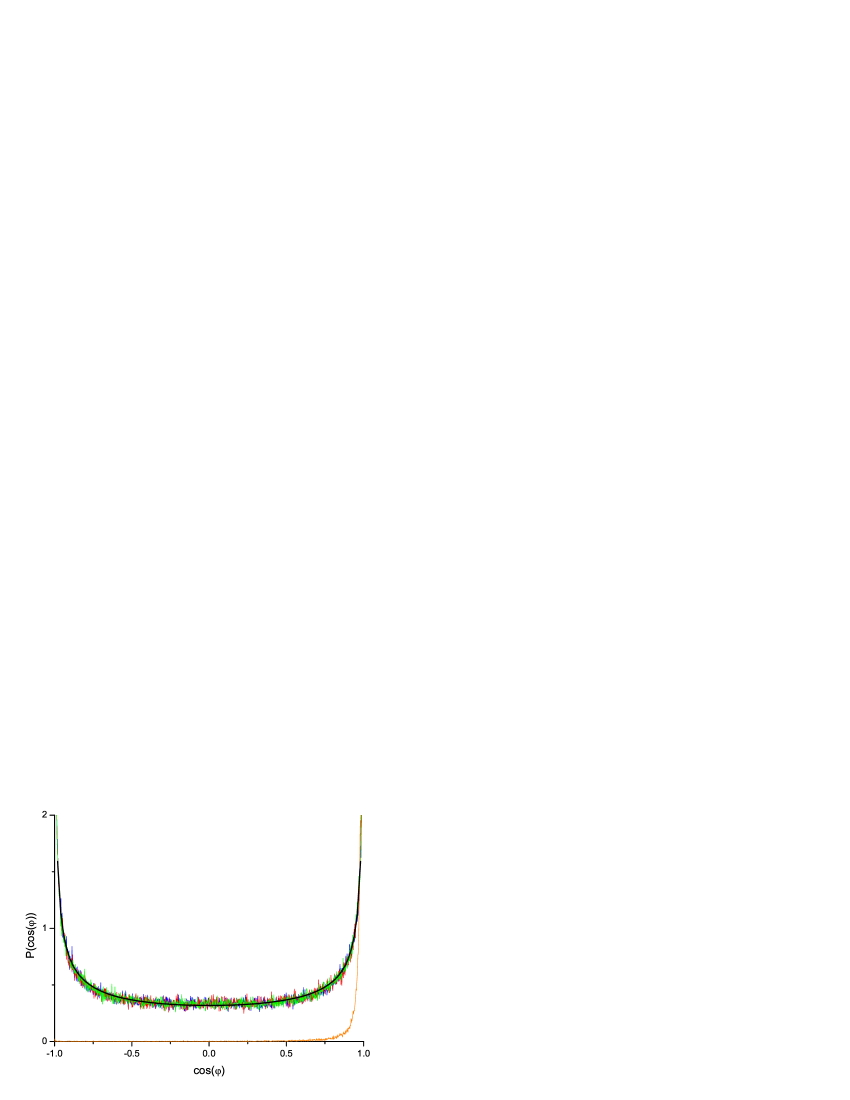
Figure 2: (color online) The distribution function of $\cos(\varphi)$ of a worm-like chain (black solid line) and of a symmetric ribbon with $a_{1}=a_{2}=0.1$, $a_{3}=0.01$ (red); $a_{1}=a_{2}=0.1$, $a_{3}=1000$ (green); $a_{1}=a_{2}=0.01$, $a_{3}=1000$ (blue). The distribution of a Fourier knot with $n_{0}=150$ is shown by the orange line.

Using the ribbon algorithm to obtain the ensemble of conformations of a ribbon with a symmetric cross section and without spontaneous curvature, we generate the corresponding distribution $P_{R}$ $\left[\cos(\Delta\varphi)\right]$. Up to numerical accuracy we find that the above distribution coincides with the simple worm-like chain expression, Eq. 19 and does not depend on the bending or twist rigidity (see Fig. 2). This concurs with our expectation that, just like worm-like chains, centerlines of ribbons can be described by freely rotating type models.
In order to generate $\infty$-smooth curves we use the Fourier knot algorithm which was originally developed with the goal of investigating knots (i.e., closed curves) Shay2 . Unlike methods based on modeling the knot as a $0$-smooth curve made of discrete, freely jointed segments Koniaris ; Deguchi ; natan ), this algorithm generates infinitely smooth knots, such that the derivatives $\left|d^{m}\vec{r}/dt^{m}\right|$ are finite for all $m$. The Fourier knot algorithm is based on the fact that for any closed curve parameterized by some arbitrary parameter $t$, the projections of the position vector $\vec{r}(t)$ on the Cartesian coordinate axes are periodic functions $r_{i}(t)=r_{i}(t+T)$ with period $T$ and can be expressed as finite Fourier sums:

$$r_{i}(t)=\sum_{n=1}^{n_{\max}}\left[A_{n}^{i}\cos(\frac{2\pi nt}{T})+B_{n}^{i}\sin(\frac{2\pi nt}{T})\right]$$ (20)

Different realizations of closed curves can be generated by choosing coefficients $A_{n}^{i},B_{n}^{i}$ from some statistical distribution. When the coefficients are given by $\lambda n^{-1}\exp{-n/n_{0}}$, where $\lambda$ are random numbers in the interval $\left[-1,1\right]$ and $n_{0}$ is an effective cutoff ($n_{0}\ll n_{\max}$), the long wavelength properties of the ensemble generated by the Fourier knot algorithm, are in good agreement with those obtained from the worm-like chain model. These properties include second moments such as the mean square distance between two points on the contour $\left\langle\left[\vec{r}(s_{1})-\vec{r}(s_{2})\right]^{2}\right\rangle$  and the tangent auto-correlation function $\left\langle\left[\vec{t}(s_{1})\cdot\vec{t}(s_{2})\right]\right\rangle$ where $\left|s_{1}-s_{2}\right|>>$ $l,$ with the persistence length $l$ determined by the cutoff as $l=0.58L/n_{0}$. However, even though the tangent auto-correlation function decays exponentially with $\left|s_{1}-s_{2}\right|$ on length scales comparable to $l$ (just like in the worm-like chain model), the corresponding decay length $l_{d}=0.435L/n_{0}\$is smaller than the persistence length obtained from the long-wavelength properties of Fourier knots. In ref. Shay2 we suggested that the ensemble of configurations generated by the Fourier knot algorithm is equivalent to a physical ensemble of polymers which possess both bending and twist rigidity and, while the short range properties of the tangent-tangent correlation function are determined by the bending persistence length only, both bending and twist persistence length control its long distance behavior. In any case, the fact that the ensemble of Fourier knots can not be characterized by a single persistence length suggests that the statistical properties of this ensemble differ from those of worm-like chains and that it is important to investigate not only the second moments but the entire distributions.
The first property we examine is the probability distribution $P_{FK}\left(\cos\Delta\varphi\right)$. As can be seen in Fig. 2, the distribution has a peak at $\cos\Delta\varphi=1,$ i.e., at $\Delta\varphi=0$. Since $\Delta\varphi=\tau\Delta s$,  we conclude that the ensemble of curves generated by the Fourier knot algorithm is characterized by finite torsion and a normal whose direction varies smoothly along the contour of each curve and, therefore, such curves can be described by the FS equation. We would like to stress that even though the torsion is described by the first three derivatives of $\vec{r}$ all of which are finite for Fourier knots, the observation that the ensemble of Fourier knots is dominated by curves with finite torsion is non-trivial since the expression for the torsion diverges at points along the contour where the curvature vanishes (see Eq. 2). Notice that for ribbons with no spontaneous curvature and twist, the partition function can be written as the product of bending and twist parts $Z=Z_{bend}Z_{twist},$ with $Z_{bend}$ is given by the functional integral (assuming a symmetric ribbon of bending persistence length $l$) rabin

$$Z_{bend} =\int D\left\{\omega_{1}\right\}\int D\left\{\omega_{2}\right\}e^{-l/2\int ds\left(\omega_{1}^{2}+\omega_{2}^{2}\right)}$$ (21)

$$=\int D\left\{\kappa\right\}\kappa e^{-l/2\int ds\kappa^{2}}.$$

Since $\omega_{1}^{2}+\omega_{2}^{2}=\kappa^{2}$, the measure $D\left\{\omega_{1}\right\}D\left\{\omega_{2}\right\}$ can be written as the product of a “radial” contribution $D\left\{\kappa\right\}\kappa\,$and an angular one. We therefore conclude that the probability of points with $\kappa\rightarrow 0$ vanishes linearly with $\kappa$ and since $\tau\propto 1/\kappa^{2}$, the torsion should be finite everywhere, as observed. Strictly speaking the above argument was derived for open ribbons and not to closed curves, but since it involves only the measure and not the form of the energy function, it applies to Fourier knots as well (see Fig. 3 where the measured distribution is plotted for Fourier knots with $n_{0}=150$).

We now turn to compare the statistical properties of $\infty$-smooth curves generated by the Fourier knot algorithm and the $1$-smooth centerlines of ribbons generated by the ribbon algorithm. Consider the probability distribution $P(R|s_{0})$ of the distance $R(s_{0})=\left|\vec{r}(s_{1})-\vec{r}(s_{2})\right|$ between points $s_{1}$ and $s_{2}$ ($s_{0}\equiv\left|s_{1}-s_{2}\right|$) along the contour (the second moment of this distribution for Fourier knots was calculated in ref. Shay2 ). The difficulty in comparing the two ensembles is that while the ribbon algorithm generates open curves, the Fourier knot algorithm yields closed loops. In order to compare the latter with the former, we make use of the fact that, as long as we consider contour distances ($s_{0})$ much shorter than the total length of the loop ($L$), $P_{FK}(R|s_{0})$ approaches the probability distribution for an open, infinitely smooth curve. In Fig. 4 we plot $P_{R}(R|s_{0})$ (ribbon) and $P_{FK}(R|s_{0})$ (knot). As expected, in the long wavelength limit ($s_{0}\gg l$) the two distributions approach the Gaussian random walk result, $P_{GRW}(R|s_{0})\propto R^{2}\exp[-3R^{2}/(4s_{0}l)]$ (see blue triangles). Since on very short length scales ($s_{0}<<l$) all distribution functions approach the trivial limit $\delta(R-s_{0}),$ the two distributions can only differ on intermediate length scales ($s_{0}\approx l)$.  This is indeed confirmed by our simulation results, Fig. 4. Notice that in this regime the maximum of $P_{FK}(R|s_{0})$ is shifted to higher values of $R$ than that of $P_{R}(R|s_{0})\$indicating that typical conformations of $1$-smooth curves are more compact than those of $\infty$-smooth ones. The origin of the difference can be traced back to the fact that the characteristic magnitude of the torsion of a $1$-smooth curve is much larger than that of an $\infty$-smooth one and, therefore, on length scales comparable to the persistence length, the latter curves are confined to a plane while the former have a three dimensional character.

V Discussion

We have demonstrated that the standard continuum models of polymers including continuous Brownian random walks, worm-like chains and ribbons, generate space curves that are not sufficiently smooth to be described by the fundamental FS equation of differential geometry. Examination of the corresponding statistical ensembles shows that the dihedral angle $\Delta\varphi$ between two successive binormals along the chain contour is uniformly distributed in the interval $[-\pi,\pi]$ and we conclude that both worm-like chains and centerlines of ribbons belong to the class of freely rotating models, with divergent torsion and discontinuous jumps of the normal to the curve. However, unlike worm-like chains, ribbons have twist rigidity which means that the rate of twist of the physical axes of the cross section remains finite everywhere along the contour of the ribbon and guarantees that the triad of unit vectors associated with the ribbon obeys the generalized FS equation familiar from the differential geometry of stripes. We compared some statistical properties of ensembles of $1$-smooth and $\infty$-smooth curves generated by the ribbon and the Fourier knot algorithms, respectively.  We showed that in the latter case the dihedral angle is peaked about $\Delta\varphi\rightarrow 0$ and, therefore, typical configurations of Fourier knots have finite torsion everywhere and can be described by the FS equation. We also compared the distribution functions of the spatial distance between two points along the contour of a ribbon and of a Fourier knot. As expected, both distribution functions approach the limiting Gaussian distribution for length scales much larger than the persistence length, but are quite different on length scales comparable to the persistence length.
Finally we would like to stress that while the physical ensembles of conformations of worm-like chains and ribbons are generated using the standard methods of statistical physics (each conformation is weighted with an appropriate Boltzmann factor, $\exp(-E/k_{b}T)$) , the ensemble generated by the Fourier knot algorithm is a purely mathematical construction and there is no elastic energy associated with different conformations of Fourier knots. Nevertheless, the observation of two persistence lengths reported in ref. Shay2 and the present finding that Fourier knots have finite torsion, suggest that the statistical properties of this mathematical ensemble (notice that persistence lengths can be measured directly from the ensemble of conformations of the space curves, just as is done in AFM experiments experiment ) are quite similar to those of a physical ensemble of conformations of polymers with both bending and torsional rigidity. The detailed exploration of this analogy is the subject of future work.

Figure 3: The distribution of curvature of Fourier knots. The solid line is a linear fit to the distribution at $\kappa\rightarrow 0$.

.

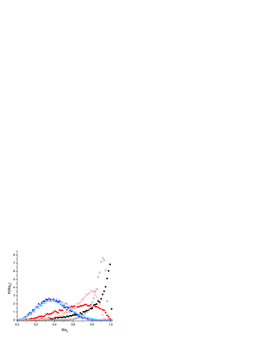
Figure 4: (color online) $P(R|s_{0})$ vs $R/s_{0}$ is plotted for Fourier knots (full symbols) and symmetric ribbons (empty symbols), of total length $L=4\pi$ and contour distance $s_{0}=L/100$. Taking the persistence length of the ribbon as $l=0.58\ast L/n_{0}$ we plot the distribution for: $n_{0}=50$, $l/s_{0}=1.16$ (black squares); $n_{0}=150$, $l/s_{0}=0.386$ (red circles); $n_{0}=600$, $l/s_{0}=0.096$ (blue triangles). The Gaussian distribution with $l/s_{0}=0.096$ is shown by the solid cyan line.