Canonical band theory of non-collinear magnetism

Abstract

A canonical band theory of non-collinear magnetism is developed and applied to the close packed fcc and bcc crystal structures. Several examples of non-collinear magnetism in the periodic table are seen to be canonical in origin. This is a parameter free theory where the crystal and magnetic symmetry, and exchange splitting, uniquely determine the electronic bands. The only contribution to the determination of magnetic stability is the change in band energy due to hybridisation resulting from spin mixing, and on this basis we are able to analyse the origin of the stability of non-collinear magnetic structures, and the instability of the FM state towards non-collinear ordering.

I Introduction

Structural trends in the periodic table are now very well understood, in contrast the situation for magnetic trends is not so clear. This can be attributed both to the fact that only a subset of the periodic table is magnetic in the three dimensional solid - the Fe group and rare earths - and also the much greater degree of freedom for magnetic ordering as compared to structural ordering. Indeed, within the transition metal block (with the exception of Mn) all elements are found either as fcc, hcp, or bcc lattices whereas a wealth of magnetic structures may be found. One has has both longitudinal and helical spin density waves, ferromagnetism, antiferromagnetism, as well as other more general non-collinear structures.

For the Fe-group metals at ambient pressure the situation is that near the centre of the series one typically finds antiferromagnetic (AFM) structures whilst near the ends ferromagnetic (FM). In between one has several metals - $\gamma$-Fe (fcc Fe), and bcc and fcc Mn - for which non-collinear structures can be found Kübler (2000). On the other hand, the late rare earth group elements are non-collinear, whilst in the middle of the series one has ferromagnetic Gd Jensen and Mackintosh (1991).

Of course, in a fully relativistic picture the magnetisation vector field will always, to some extent, be non-collinear. However, for the Fe-group and rare earths this leads only to intra-atomic non-collinearity and not to the coarse grained inter-atomic non-collinearity where the average moments associated with different sites point in different directions.

The richness of magnetic structures means that most theoretical approaches focus on specific materials, and only a few attempts have been made to determine conditions whereby one places possible magnetic structures in some general scheme. A notable early attempt along such lines was the work of Pettifor Pettifor (1980) who, on a similar basis to Friedel’s theory for the stability of crystal structures, formulated a phase diagram in terms of the Stoner parameter to the band width $I/W$ and the $d$-band occupation number. In this theory the ferromagnetic and disordered local moment structures were considered, and the phase diagram revealed a simple argument as to why bcc Fe is a good local moment system, but fcc Co and fcc Ni are not. Heine and Samson Heine and Samson (1983), again using arguments based on generalised Stoner criteria constructed a similar phase diagram diagram but included also the AFM structure. They further made actual calculations of the generalised Stoner $I$ within the tight binding approximation, showing how $\gamma$-Fe was placed at the crossing point of the AFM and FM stability criteria, and hence was likely to assume a non-collinear structure. Hirai, Hirai (1982) on the basis of an approximation to Hartree-Fock theory, calculated the energy of FM, AFM, and helical spin spiral structues as a function of an intra-atomic parameter and the $d$-band occupation number. The resulting phase diagram showed the appearence of a region of helical stability inbetween regions of FM and AFM stability. Unfortunately, the electronic structure in the Hartree-Fock approximation is known to be drastically in error compared to experiment.

Recently, an attempt was made to re-examine the issue of non-collinear stability on the basis of first principle calculations Lizárraga et al. (2004). Interestingly, it was found that materials collinear at their equlibrium moment were non-collinear for smaller (local) moments, induced either by pressure or a fixed spin moment procedure. On this basis, it was speculated both that any magnetic material could be made non-collinear and also that the primary factor governing the instability of the FM state towards a non-collinear state was the hybridisation of crossing spin-up and spin-down bands at the Fermi level. However, in contrast to previous approaches no attempt was made to link this to the $d$-band occupation.

The purpose of the present article is to unify the spirit of the earlier works, where the emphasis was upon finding general magnetic phase diagrams, with the approach in Ref. Lizárraga et al., 2004 where the importance of spin hybridisation for specific magnetic structures was emphased. As we shall show, this can be accomplished on the basis of Andersen’s canonical $d$-band theory Andersen (1975); Andersen and Jepsen (1977), suitably generalised to deal with non-collinear magnetism. It has been shown in the past that canonical $d$-band theory gives a good qualitative account of crystal stability in the transition metal block and rare earths Andersen and Jepsen (1977); Skriver (1985), even including the impact of collinear magnetism upon crystal stability Söderlind et al. (1994); Abrikosov et al. (1996). Until now, however, it has not been used to investigate non-collinear magnetic stability.

The remainder of this article is structured as follows. In Section II we describe canonical band theory and its generalisation to deal with non-collinear magnetism, followed in Section III by details pertinent to its implementation. In Section IV we present non-collinear magnetic phase diagrams for the close packed lattices, and in Section V discuss the reasons for non-collinear stability. Finally, in Section VI we conclude.

II Non-collinear canonical band theory

Within the Linear Muffin Tin Orbital electronic structure method in the atomic sphere approximation (LMTO-ASA) the electronic bands are given by the secular equation

$$[P_{L^{\prime}L}(E)\delta_{l^{\prime}m^{\prime}lm}-S_{L^{\prime}L}({\bf k})]a_{i{\bf k}}=0$$ (1)

where $L=(lm)$ are angular momentum indices, ${\bf k}$ a reciprocal lattice vector, and $i$ a band index. This equation has the remarkable feature that it is split into a part which depends solely on the one-electron potential for the given atomic species, $P_{L^{\prime}L}(E)$, known as the potential function, and a part which depends only on the crystal symmetry, the structure matrix $S_{L^{\prime}L}({\bf k})$. Neglecting the off diagonal $l^{\prime}l$ blocks of the structure matrix, which amounts to neglecting all hybridisation effects between different angular momentum chanels, leads to a set of pure $l$ canonical bands given by $P_{li}=S_{li}({\bf k})$ unique for each crystal structure. In cases where the physics of the $d$-band is expected to play a leading role one can further neglect all but the $l^{\prime}=l=2$ block and by approximating the potential function by $P=(E-C)/(\mu S^{2})$ find a simple eigenvalue problem for the canonical $d$-bands

$$[(\epsilon_{i{\bf k}}-C)/(\mu S^{2}){\bf 1}-{\bf S}({\bf k})]a_{i{\bf k}}=0$$ (2)

where $1\leq i\leq 5$. One should note that since $C$ is the $d$-band centre and $1/(\mu S^{2})$ simply sets the energy scale, this is a parameter free theory.

To develop a non-collinear magnetic generalisation one first must specify a particular class of magnetic structures. It is convenient to consider helical spin spiral structures, since these contain both the FM and AFM structures as limits. In a helical spin spiral structure the magnetisation is given by

$$m({\bf R}_{n})=(\sin\theta\cos({\bf q}.{\bf R}_{n}),\sin\theta\sin({\bf q}.{\bf R}_{n}),\cos\theta)$$ (3)

with ${\bf R}_{n}$ a direct lattice vector and ${\bf q}$ a reciprocal lattice vector. Although this structure may be incommensurate with the underlying lattice, it is invarient under a lattice translation ${\bf R}_{n}$ and a rotation about the spiral axis by ${\bf q}.{\bf R}_{n}$. This leads to a generalised Bloch theorem and an LMTO-ASA secular equation. By deploying the canonical procedure outlined above one finds an eigenvalue problem for the canonical bands of the spin spiral given by

$$[(\epsilon_{i{\bf k}\sigma}-C)/(\mu S^{2}){\bf 1}-({\bf S}({\bf k})+{\bf\Delta})]a_{i{\bf k}\sigma}=0$$ (4)

where

$${\bf S}({\bf k})=\left(\begin{array}[]{cc}{\bf S}^{+}+{\bf S}^{-}\cos\theta&{\bf S}^{-}\sin\theta\\ {\bf S}^{-}\sin\theta&{\bf S}^{+}-{\bf S}^{-}\cos\theta\end{array}\right)$$ (5)

and $S_{m^{\prime}m}^{\pm}=S_{m^{\prime}m}^{{\bf k}+{\bf q}/2}\pm S_{m^{\prime}m}^{{\bf k}-{\bf q}/2}$, and also

$${\bf\Delta}=\left(\begin{array}[]{cc}\Delta/2&0\\ 0&-\Delta/2\end{array}\right)$$ (6)

. Eq. 4 determines a set of bands unique for each symmetry of the spin space group.

To complete the theory one needs to determine the canonical moment $m$ projected onto the local quantisation axis, for a given exchange splitting. This may be extracted by evaluating the expectation value of $\sigma_{z}$ over the canonical wave function which leads to the natural result

$$m=\sum_{i{\bf k}}^{occ}(|a_{i{\bf k}\uparrow}|^{2}-|a_{i{\bf k}\downarrow}|^{2})$$ (7)

and where the sum is over all occupied states. Together with the $d$-band occupation number $n$ and the one-electron energy $e$, given respectively by

$$n = \sum_{i{\bf k}\sigma}^{occ}|a_{i{\bf k}\uparrow}|^{2}$$

$$e = \sum_{i{\bf k}\sigma}^{occ}|a_{i{\bf k}\sigma}|^{2}\epsilon_{i{\bf k}\sigma}$$ (8)

these form the basic quantities of the theory. However, in order to determine the stability of competing magnetic structures for a given $n$ and $m$ what one needs is not the one-electron energy but the kinetic energy. This is due to the fact that in a canonical theory there is no intrinsic intra-atomic force causing the magnetisation, but rather it is imposed by setting the exchange splitting to some finite value which thus plays the role of an external field. The contribution of the energy of this external field is included in the one-electron energy and so must be subtracted, which leaves the kinetic energy of the one-electron system

$$T=e-\int_{0}^{m}\Delta(m)dm$$ (9)

as the quantity to be used for comparing the stability of different magnetic structures.

III Computational details

In order to solve Eqs. 4 to II we use a Monkhurst-Pack mesh with 18900, 109800, 216000, and 37820 ${\bf k}$-points in the irreducable Brillouin zone for the FM structure, and spirals along $\Gamma X$, XW and WL, and LG respectively. For the bcc irreducable Brillouin zone we use 5200, 28830, and 109800 ${\bf k}$-points for the FM structure and spirals along $\Gamma$H, and HP respectively. For the ${\bf k}$-integration in Eqs. 7 and II we use an eigenvalue broadening of 4.5mRy. For the potential parameters which, for the canonical $d$-band theory, simply set the origin and scale of energy we set $C=0$ and take $1/(\mu S^{2})$ for non-magnetic fcc Fe.

One should note that the natural variables of the theory outlined above are the Fermi energy $E_{F}$ and the exchange splitting $\Delta$. However, the physical variables for determining magnetic stability are the $d$-band occupation number $n$ and the spiral local moment $m$. Thus we need to solve $n^{\prime}(E_{F},\Delta,{\bf q})=n$ and $m^{\prime}(E_{F},\Delta,{\bf q})=m$ to find the values of $E_{F}$ and $\Delta$ that give the required $n$ and $m$. This can easily be done by minimising a function defined as

$$f=[n^{\prime}(E_{F},\Delta,{\bf q})-n]^{2}+[m^{\prime}(E_{F},\Delta,{\bf q})-m]^{2}.$$ (10)

In order to facilitate this it is convenient to pre-calculate the functions $n^{\prime}$, $m^{\prime}$, and also the corresponding one-electron energy function $e^{\prime}(E_{F},\Delta,{\bf q})$ over the full range of $E_{F}$ and $\Delta$ and interpolate using cubic splines. In this way one can very rapidly minimise Eq. 10, whereas if $n^{\prime}$ and $m^{\prime}$ are repeatedly calculated by solving Eq. 4 over the Brillouin zone this would be a very slow procedure.

IV Canonical phase diagrams

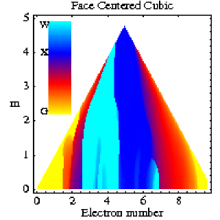
Figure 1: Canonical phase diagram for $\Gamma XW$ spin spirals in the fcc structure.

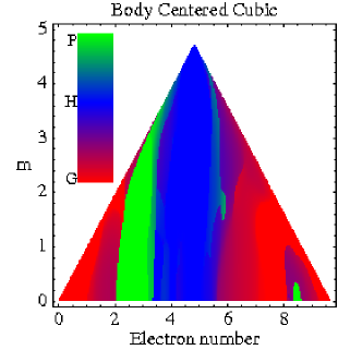
Figure 2: Canonical phase diagram for $\Gamma HP$ spin spirals in the bcc structure.

In Figs. 1 and 2 we show the calculated phase diagrams when one considers spin spirals along the $\Gamma XW$ symmetry lines of the fcc Brillouin zone and the $\Gamma HP$ lines of the bcc Brillouin zone. In order to construct these phase diagrams we have used planer spin spin spirals, $\theta=\pi/2$ in Eq. 3, since then AFM structures are limits of spin spirals. In fact, for single basis crystal structures like fcc and bcc, all points of the BZ boundary correspond to AFM structures.

One can notice immediately that, as expected, near half filling of the $d$ band one finds AFM structures while for the nearly fully occupied or empty $d$-band one finds ferromagnetism. Unfortunately, the correspondence with the $d$ electron numbers of the transition metals is only approximate, since the region of FM is too small in both the fcc and bcc phase diagrams. For instance, in the fcc phase diagram FM is the stable solution for $n>8.8$, whereas since fcc Co is FM the boundary should be $n\approx 8.0$.

In Ref. Lizárraga et al., 2004 it was noted that fcc Co developed a spin spiral structure along the $\Gamma X$ direction if the moment was reduced from its equlibrium value to 0.8 $\mu_{B}$. In fact, as one can see from Fig. 1 this is what happens in the canonical picture as well: there is a transition from FM stability to a spin spiral in the $\Gamma X$ direction as the moment is reduced for $n\approx 8.8$. Interestingly, reducing the value of $n$ continuously increases this splitting about the $\Gamma$ point so that it becomes a spiral with ${\bf q}=[0,0,0.5]$, which is exactly the spin spiral structure observed for $\gamma$-Fe in calculations. In fact, in the fcc phase diagram it can be seen that there is quite a large region where this spiral is stabilised. Furthermore, by lowering the moment for $n\approx 6.5$ this spiral closes about the $X$ point until one finds nearly degenerate spin spirals along the $\Gamma X$ and $XW$ symmetry lines, again as is seen in self-consistent calculations. Thus one can see that the formation of small moment spin spirals for larger $n$ moves continuously to the intermediate moment spin spiral of $\gamma$-Fe before finally the $X$ AFM structure becomes stable near half filling. This is an appealing picture, since it unites the results of Ref. Lizárraga et al., 2004 into a general magnetic phase diagram for the fcc structure. In Fig. 3 are shown the spin spiral spectrum’s corresponding to the various magnetic phases discussed.

For the bcc structure, shown in Fig. 2 one can note that the region of stability for the FM structure is much larger, which makes sense since bcc Fe is ferromagnetic whereas $\gamma$-Fe is non-collinear. However, as for the fcc lattice the region of FM stability is too small. Interestingly, at $n\approx 9.0$ one finds an incursion of non-collinear structures for small moments. Again, this is what is seen in Ref. Lizárraga et al., 2004, where bcc Ni becomes non-collinear for small moments.

Finally, one can note the approximate symmetry of both the fcc and bcc magnetic phase diagrams about half filling. This is interesting since, as was already mentioned, the late rare earths all assume a non-collinear structure. Since for these metals the $f$ electrons are localised and simply play the role of polarising the itinerent $spd$ electrons one might expect that again the crucial parameters for describing their magnetism would be the $d$-band electron number and moment $m$. In fact, this is exactly what happens for the structural energies where for $1.5\leq n\leq 2.0$ one finds the sequence of rare earth structures Skriver (1985). The symmetry seen in Figs. 1 and 2 is suggestive of the fact that there is a connection between the late rare earths and the late Fe-group elements with artifically lowered moments. However, in contrast to the canonical crystal energy differences, the magnetic canonical theory is not sufficiently quantitative to give the actual non-collinear structures of the rare earths, and therefore we have not shown the hcp phase diagram.

For a more quantitative theory, the effect of angular momentum hybridisation must be included, but in this case it is no longer a parameter free theory, since band centres, band distortions, and band widths must be introduced for the $l=0,1,2$ chanels.

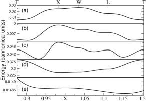
Figure 3: Canonical spin spiral spectrum’s for the symmetry path $\Gamma$XWL$\Gamma$ in the fcc Brillouin zone. Shown are spectrums for (a) $n=9.3$, $m=0.5$, (b) $n=8.8$, $m=0.4$, (c) $n=7.5$, $m=1.2$, and (d) $n=0.5$, $m=3.3$. Shown in the lowest panel is (e) the region around the X point for $n=6.5$, $m=0.8$. The top scale refers to graphs (a)-(d), and the bottom to graph (e).

V Origin of stability of non-collinear structures

Figure 4: Canonical Density of States for the (a) ferromagnetic, (b) ${\bf q}=[0.0,0.0,0.5]$ spin spiral, and (c) antiferromagnetic X-point structure.

It is interesting to first reconsider the arguments for the stability of the collinear AFM and FM structures. The reason for the existance of AFM near half filling and FM for the nearly full band is well known and has been described by a number of authors (see Ref. Kübler, 2000 and references therein). The hybridisation between the different sublattices of the AFM structure, equivalent to the hybridisation from spin mixing when the AFM structure is considered as the limit of a planer spin spiral, opens a large pseudo-gap in the density of states. It is this which stabilises the AFM structure at half filling. The argument is thus couched in terms of significant movements of spectral weight at all energies, and not to changes at only the Fermi level. In Fig. 4 are shown the density of states (DOS) for the FM, X point AFM, and spin spiral ${\bf q}=[0.0,0.0,0.5]$ structures for the fcc lattice. As can be seen the structure of the spiral DOS is somewhere between that for the FM and AFM structures. Thus the occurance of non-collinear stability between the FM and AFM regions can be understood by the same reasoning that explains the placement of the FM and AFM regions themselves.

It is natural that the determination of the lowest energy magnetic structure will, in general, come about as the result of movements of spectral weight at all energies since generally spin hybridisation will be very significant. On the other hand, it is not immediately clear that this will be the case when one considers the instability of the FM state towards non-collinear structures. In Ref. Lizárraga et al., 2004 it was speculated that such instabilities are driven by the hybridisation of crossing spin-up and spin-down bands at the Fermi level. This is, of course, the classic picture when one has the situation of Fermi surface nesting, as happens in the late rare earths. There it is the Fermi surface of the non-magnetic state which shows nesting and this is relevent to the final magnetic state since the itinerant $spd$ moment is very small (0.2-0.6 $\mu_{B}$). However, the argument presented in Ref. Lizárraga et al., 2004 is that the number of spin-up and spin-down band crossings at the Fermi energy may more generally hold the key to understanding the instability of the ferromagnetic state towards a non-collinear state.

The stability or otherwise of the FM state is given by the eigenvalues of the Hessian of the FM point in a general energy space of magnetic structures. For the magnetic structures considered in this work, this could be determined either as a $\theta\rightarrow 0$ limit for a finite ${\bf q}$ or alternatively as a ${\bf q}\rightarrow[0,0,0]$ limit for finite $\theta$. To investigate the origin of the instabilty of the FM state towards non-collinearity we choose to investigate the energy difference of the FM structure with the ${\bf q}=[0.0,0.0,0.1]$ spin spiral. This will be positive if the FM structure is stable, and negative otherwise. If the arguments of Ref. Lizárraga et al., 2004 are relevent then this energy difference should be dominated by the contribution from a window near the Fermi energy.

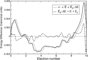
Figure 5: Energy difference of FM and ${\bf q}=[0.0,0.0,0.1]$ spin spiral structures. Full line is total energy different whilst caption indicates components.

In Fig. 5 is plotted the energy difference of the FM and ${\bf q}=[0.0,0.0,0.1]$ structures for the fcc lattice as a function of band filling for a fixed exchange splitting of $\Delta=0.3$. This leads to a path in the (n,m) phase diagram with $m$ almost at the saturation value for each $n$ (at half filling $m=4.2$). Also shown in Fig. 5 is a breakdown of the energy into that arising from a small window near the Fermi energy, with $\Delta E=$ 0.015, and that from the remaining spectrum. One can clearly see that it is this energy and not that arising from the Fermi energy window which follows the total energy difference. In fact, while the indication of FM stability from the total energy difference is in agreement with what one would expect from the phase diagram in Fig. 1, the Fermi window energy difference shows no correspondence to it. One can also notice that the energy difference has exactly two crossing points. This is in line with the theorem of Heine and Samson Heine and Samson (1980) stating that any property of a tight binding band must have at least two crossing points as a function of band filling. A similar picture is found for other settings of the exchange splitting.

It would appear then that there is no special significance attached to spin hybridisation at the Fermi level in considering the stability of the FM state. This makes sense when one considers that, for a given band filling, if the hybridisation arising from solely around the Fermi level dominated, then the corresponding change for some lower energies must integrate to zero. This could only be the case if the change in band structure from hybridisation is exactly symmetric. This cannot, of course, be the case for all energies i.e. for all $d$-band electron numbers. Thus, in general, it is hybridisation changes for all energies that determine even the stability criteria of the FM state towards non-collinearity.

VI Conclusions

To conclude a generalisation of Andersen’s canonical band theory has been used to derive magnetic phase diagrams for the close packed bcc and fcc structures. One finds that a number of the non-collinear structures observed in self-consistent calculations are found, but that the phase diagrams are in error for moments near saturation and the regions of ferromagnetic stability are too small. This is most likely due to the missing hybridisation between different angular momentum chanels. A similar situation arises in the case of crystal stability where errors found in the $d$-band canonical theory are removed by inclusion of $s$ and $p$ states Skriver (1985).

An analysis of the canonical magnetisation energetics in terms of contributions from different energy windows, shows that, generally, it is hybridisation from the whole spectrum which acts to determine the stability of the ferromagnetic state with regard to non-colliear magnetism. Thus the picture of band crossing at the Fermi level emphased in Ref. Lizárraga et al., 2004 does not appear to be relevant for the determination of the stability of the ferromagnetic state.